Article

Fixed-Time Adaptive Tracking Control for a Quadrotor Unmanned Aerial Vehicle with Input Saturation

School of Electronic and Information Engineering, Suzhou University of Science and Technology, Suzhou 215009, China
*
Author to whom correspondence should be addressed.
Actuators 2023, 12(3), 130; https://doi.org/10.3390/act12030130
Submission received: 19 February 2023 / Revised: 9 March 2023 / Accepted: 16 March 2023 / Published: 18 March 2023
(This article belongs to the Section Control Systems)

Abstract

:
Considering the problem of tracking control for a quadrotor unmanned aerial vehicle (QUAV) with input saturation, parameter uncertainties and external disturbances, a command filtered backstepping-based fixed-time adaptive control scheme was developed. The problem of “explosion of complexity” (EOC) is tackled by utilizing the fixed-time command filter, and the influence of filtered error is removed based on the fractional power-error-compensation mechanism. A fixed-time auxiliary system was designed to compensate for the input saturation of the QUAV. It strictly proves that the closed-loop system signals are fixed-time bounded, and the tracking errors converge to a sufficiently small region near the origin in a fixed time, and the convergence time is independent of the initial states. Finally, the effectiveness of the proposed fixed-time adaptive control algorithm is demonstrated via a numerical simulation.

1. Introduction

Quadrotor unmanned aerial vehicles (QUAVs) have outstanding advantages, such as low cost, accurate hovering, and maneuverability, and they play a key role in the fields of cargo transportation, high-altitude photography, and military reconnaissance [1]. Nevertheless, QUAV is a class of multi-input and multi-output system with six degrees of freedom and four independent inputs [2], which has typical characteristics, including high nonlinearity, underactuation, and strong coupling [3]. Thus, the research on high-performance control for the QUAV has gradually become a hot spot.
In recent years, all sorts of flight control algorithms have been developed for the QUAV—for example, sliding mode control [4], backstepping control [5], dynamic surface control [6], and adaptive control [7]. For a QUAV with external disturbances and system uncertainties, an adaptive sliding mode control scheme was designed in [8]. However, the chattering problem is the main shortcoming of the aforesaid sliding mode control strategies. Based on the backstepping design method, in [9], an adaptive trajectory tracking control algorithm was developed for the QUAV with prescribed performance. It is worth noting that the virtual control signals need to be differentiated several times in the standard backstepping design process, which leads to the problem of “explosion of complexity” (EOC). By means of the dynamic surface control approach, a prescribed performance control strategy was proposed for the QUAV in [10], where the problem of EOC was addressed via a first order filter. Nevertheless, the influence of filtered error was not considered in those dynamic surface control schemes, and the performance of the QUAV will decline to a certain extent. Fortunately, the command filtered backstepping technique was first proposed in [11], such that the problem of EOC and the influence of filtered error can be eliminated simultaneously. Considering the QUAV with sensor faults, a command filtered backstepping-based fault-tolerant control strategy was presented in [12]. By fusing the command filtered backstepping method, an active anti-disturbance flight-control algorithm was designed in [13].
It should be mentioned that many asymptotically convergent control schemes of the QUAV require infinite time to realize accurate trajectory tracking, which is impractical for engineering applications. Recently, the finite-time stability theory was established in [14] for equilibrium of continuous autonomous systems. Although various finite-time control schemes [15,16,17] have been developed for QUAV, the convergence time heavily depends on the initial states. If the initial states of the QUAV are not accurately available, the finite-time control method will fail. Fortunately, the fixed-time stability theory was first proposed in [18], which guarantees that the upper bound of convergence time does not depend on the initial states and is only in connection with the control parameters. Subsequently, the fixed-time stability theory has been successfully employed for robotic systems [19], surface vehicles [20], and rigid spacecraft [21], whose outstanding advantage is that the system can be stabilized to the equilibrium in a fixed time without the information of initial conditions. A fixed-time output-feedback control algorithm was proposed in [22], where the fixed-time state observer was designed to estimate unavailable velocity states and unknown uncertainties. Similarly, in [23], a fixed-time observer-based safety control scheme was developed for the QUAV with actuator faults and disturbances. To guarantee the transient performance of the QUAV, a fixed-time prescribed performance adaptive trajectory tracking algorithm was proposed in [24]. By fusing fixed-time stability theory and the sliding mode control technique, in [25], the attitude tracking problem of the QUAV was addressed within a fixed time.
Note that the input saturation of the QUAV is unavoidable owing to the limitation of battery energy or physical structure. If no effective methods are used to cope with this problem, system instability and flight accidents will worsen. Current approaches to solving the input saturation mainly include the smooth function to approximate the saturation nonlinearity [26] and the auxiliary system to compensate for the saturation’s influence [27]. Considering the QUAV is subject to wind perturbation and model uncertainty, a finite-time sliding mode control scheme was proposed in [28], where a compensation system was used to address the input saturation. By means of the dynamic surface control approach and auxiliary system, a distributed output feedback anti-saturation formation control algorithm was presented in [29]. To the best of authors’ knowledge, there are few efforts to study the fixed-time adaptive tracking control problem for a QUAV with input saturation, which motivated our present study.
Based on the above discussion, this article proposes a fixed-time adaptive control scheme for the QUAV with input saturation, parameter uncertainties, and external disturbances under the command-filtered backstepping design framework. The main contributions are given as follows.
(1)
In contrast to backstepping control strategies [5,9] and dynamic surface control schemes [6,10], a fixed-time command filter can be constructed to address the problem of EOC, and the influence of filtered error is removed by the fractional power-error compensation mechanism within a fixed time.
(2)
Unlike the existing finite-time control algorithms [15,16,17], the designed fixed-time adaptive control scheme ensures that the tracking errors of the QUAV converge to a sufficiently small region near the origin in a fixed time, and the convergence time is independent of the initial states.
(3)
Differently from the traditional anti-saturation control strategies for the QUAV [28,29], an auxiliary system with fixed-time convergence is designed to compensate for the effect of input saturation within a fixed time, which is more useful in practice.
The rest of this paper is given as follows. The problem formulation and preliminaries are shown in Section 2. The main results, including fixed-time adaptive controller design and stability analysis, are presented in Section 3. The simulation results in Section 4 demonstrate the effectiveness of the developed fixed-time control algorithm. Section 5 gives the conclusions.

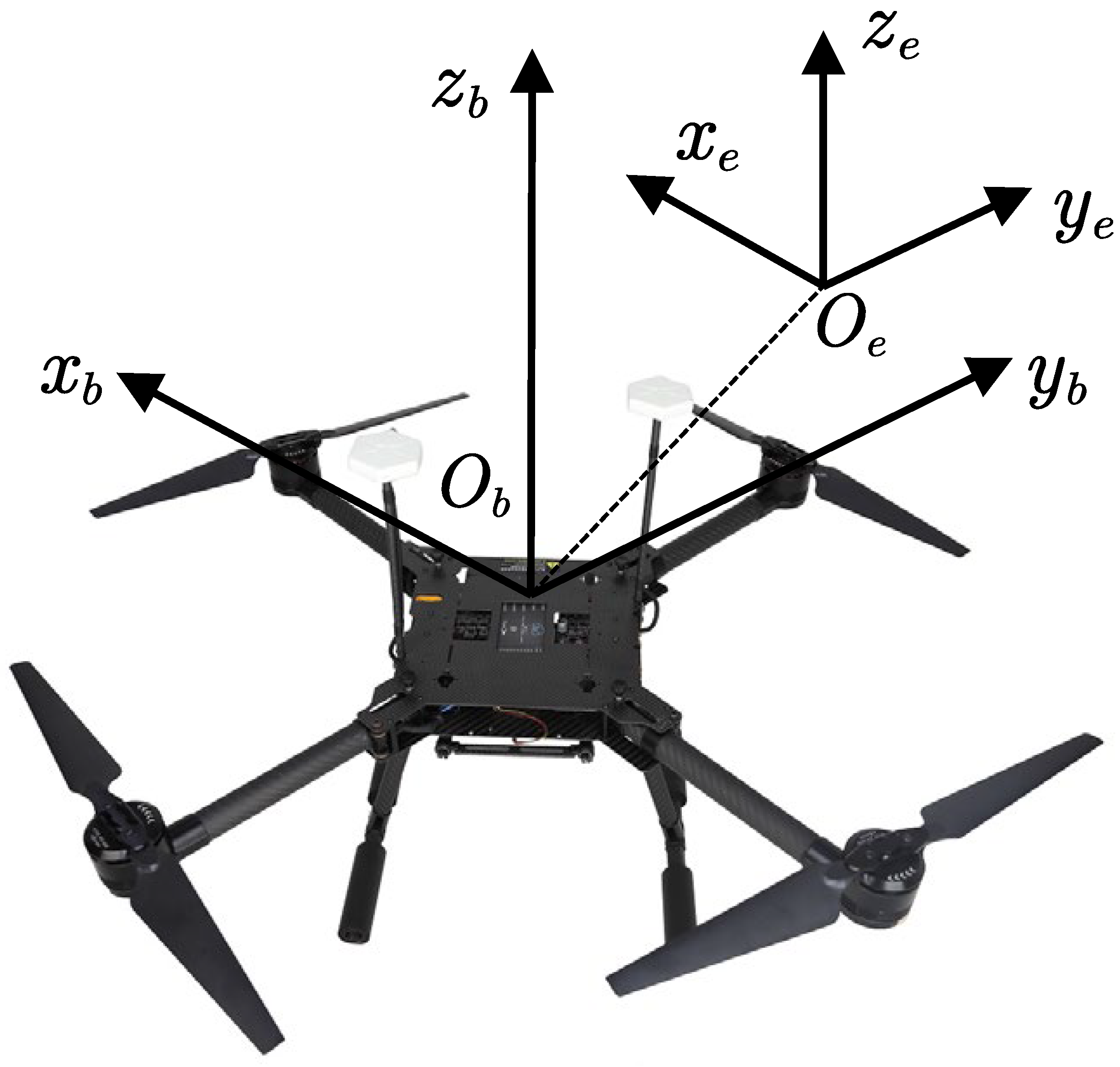
2. Problem Formulation and Preliminaries

The QUAV has six degrees of freedom in space and can either move linearly along or rotate around three-coordinate axes. Define two coordinate systems, including the Earth coordinate system E = { O e , x e , y e , z e } and the body coordinate system B = { O b , x b , y b , z b } . The corresponding rotation matrix is denoted as R 1 : B E . O b is the center of mass, and the structure of the QUAV is presented in Figure 1. Rotation matrix R 1 indicates the linear velocity relationship between body coordinate system and Earth coordinate system, which is given as
R 1 = C θ C ψ S ϕ S θ C ψ C ϕ S ψ C ϕ S θ C ψ + S ϕ S ψ C θ S ψ S ϕ S θ S ψ + C ϕ C ψ C ϕ S θ S ψ S ϕ C ψ S θ S ϕ C θ C ϕ C θ
and R 2 is defined as the transfer matrix from a body-fixed to an Earth-fixed coordinate system, which is expressed as
R 2 = 1 S ϕ T θ C ϕ T θ 0 C ϕ S ϕ 0 S ϕ / C θ C ϕ / C θ
where C ( · ) cos ( · ) , S ( · ) sin ( · ) and T ( · ) tan ( · ) .
Based on the Newton–Euler formula, the dynamics of the QUAV are given as
X ˙ = ν m ν ˙ = u F R 1 E m g E F X X ˙ + d X Θ ˙ = R 2 Ω J Ω ˙ = U Θ Ω × J Ω F Θ Θ ˙ + d Θ
where E = [ 0 , 0 , 1 ] .
Considering the cases of small angle change and input saturation, Equation (1) is rewritten as
X ˙ = ν ν ˙ = G 1 Φ 1 ( U X ) g E + f 1 + d 1 Θ ˙ = Ω Ω ˙ = G 2 Φ 2 ( U Θ ) + f 2 + d 2
where G 1 = m 1 , G 2 = J 1 , f 1 = m 1 F X X ˙ = [ f 1 , 1 , f 2 , 1 , f 3 , 1 ] , f 2 = J 1 Ω × J Ω J 1 F Θ Θ ˙ = [ f 1 , 2 , f 2 , 2 , f 3 , 2 ] , d 1 = m 1 d X = [ d 1 , 1 , d 2 , 1 , d 3 , 1 ] , and d 2 = J 1 d Θ = [ d 1 , 2 , d 2 , 2 , d 3 , 2 ] . Φ 1 ( U X ) = [ sat ( u x ) , sat ( u y ) , sat ( u z ) ] and Φ 2 ( U Θ ) = [ sat ( u ϕ ) , sat ( u θ ) , sat ( u ψ ) ] are the control inputs with saturation nonlinearity, where u x = u F ( C ϕ S θ C ψ + S ϕ S ψ ) , u y = u F ( C ϕ S θ S ψ S ϕ C ψ ) , u z = u F C ϕ C θ , and
sat ( u i ) = Φ i , L , u i < Φ i , L u i , Φ i , L u i Φ i , R , i = x , y , z , ϕ , θ , ψ . Φ i , R , u i > Φ i , R
with Φ i , L < 0 and Φ i , R > 0 being constants, and U X = [ u x , u y , u z ] is the control input of the position subsystem.
Control Objective: This paper aims to design a fixed-time adaptive control scheme for the QUAV with input saturation, which ensures that the closed-loop system signals are fixed-time bounded, and the tracking errors converge to a sufficiently small region near the origin in a fixed time.
Assumption 1.
The QUAV flies at a low speed and a small angle. Assume that all states of the QUAV are available, and ϕ ( π / 2 , π / 2 ) , θ ( π / 2 , π / 2 ) hold.
Assumption 2.
The desired signals x d , y d , z d , ψ d and their first-order derivatives x ˙ d , y ˙ d , z ˙ d , ψ ˙ d are known and bounded.
Assumption 3.
The external disturbances d 1 = [ d 1 , 1 , d 2 , 1 , d 3 , 1 ] and d 2 = [ d 1 , 2 , d 2 , 2 , d 3 , 2 ] are continuous and bounded; i.e., | d i , s | d ¯ i , s , d ¯ i , s > 0 ,   i = 1 , 2 , 3 , s = 1 , 2 .
Lemma 1.
[30] Suppose that F ( x ) is a continuous function defined on a compact set Ω. For any given constant ε > 0 , there exists a fuzzy logic system φ S ( x ) such that
sup x Ω F ( x ) φ S ( x ) ε
where φ = φ 1 , φ 2 , , φ n denotes the ideal weight vector; S ( x ) = [ S 1 ( x ) , S 2 ( x ) , , S n ( x ) ] / i = 1 n S i ( x ) is the basis function vector with n being the number of the fuzzy rules, and S i ( x ) = exp x μ ¯ i x μ ¯ i v ¯ i 2 with μ ¯ i = [ μ ¯ i , 1 , μ ¯ i , 2 , , μ ¯ i , N ] being the center vector and v ¯ i being the width.
Lemma 2.
[31] For m > 0 , n > 0 , and the real-valued function Λ ( x , y ) > 0 , one obtains
| x | m | y | n m Λ ( x , y ) | x | m + n m + n + n Λ ( x , y ) m n | y | m + n m + n .
Lemma 3.
[32] For a 0 , b > 0 , c > 0 , k > 0 , l k , and ρ > 1 , one has
a c ( b a ) 1 1 + c ( b 1 + c a 1 + c ) ( l k ) ρ l ρ k ρ .
Lemma 4.
[33] For i = 1 , , n , C i R , 0 < p ¯ 1 , and q ¯ > 1 , one obtains
i = 1 n C i p ¯ i = 1 n C i p ¯ n 1 q ¯ i = 1 n C i q ¯ i = 1 n C i q ¯ .
Lemma 5.
[34] Consider a system ξ ˙ = ϝ ( ξ ) , ξ ( 0 ) = ξ 0 . If there exists a continuous positive definite function V and constants λ 1 > 0 , λ 2 > 0 , ι > 0 , 0 < α < 1 , and β > 1 , such that V ˙ ( ξ ) λ 1 V α ( ξ ) λ 2 V β ( ξ ) + ι , the system is practical fixed-time stable, and the convergence time is calculated as
T T m a x = 1 λ 1 ϖ ( 1 α ) + 1 λ 2 ϖ ( β 1 )
where 0 < ϖ < 1 , and ξ finally converges to the compact set
ξ V ( ξ ) min ι λ 1 ( 1 ϖ ) 1 α , ι λ 2 ( 1 ϖ ) 1 β .

3. Main Results

Define the tracking errors as follows:
e 1 = X X d = [ e 1 , 1 , e 2 , 1 , e 3 , 1 ]
e 2 = ν ν ¯ d = [ e 1 , 2 , e 2 , 2 , e 3 , 2 ]
e 3 = Θ Θ d = [ e 1 , 3 , e 2 , 3 , e 3 , 3 ]
e 4 = Ω Ω ¯ d = [ e 1 , 4 , e 2 , 4 , e 3 , 4 ]
where X d = [ x d , y d , z d ] and Θ d = [ ϕ d , θ d , ψ d ] are the desired position and attitude signals of the QUAV, and ϕ d and θ d will be given later. ν ¯ d = [ ν ¯ 1 , 1 , ν ¯ 2 , 1 , ν ¯ 3 , 1 ] and Ω ¯ d = [ Ω ¯ 1 , 2 , Ω ¯ 2 , 2 , Ω ¯ 3 , 2 ] are the output signals of the virtual control signal. ν d = [ ν 1 , 1 , ν 2 , 1 , ν 3 , 1 ] and Ω d = [ Ω 1 , 2 , Ω 2 , 2 , Ω 3 , 2 ] are taken as the inputs of the fixed-time command filter. The fixed-time command filter is designed as
N 1 ˙ = R 1 ι 1 ( σ ) + N 2 N 2 ˙ = R 2 ι 2 ( σ )
where N 1 and N 2 are the state variables; ι 1 ( σ ) = sig ( σ ) 1 / 2 + μ sig ( σ ) 3 / 2 , ι 2 ( σ ) = 1 2 sign ( σ ) + 3 2 μ 2 sig ( σ ) 2 + 2 μ σ , sig ( σ ) γ = | σ | γ sign ( σ ) , γ = 1 2 , 3 2 , 2 , σ = N ¯ i , s N i , s , N = ν , Ω , N ¯ = ν ¯ , Ω ¯ , i = 1 , 2 , 3 , and s = 1 , 2 ; R 1 , R 2 , and μ are the filtering constants.
Define the compensated tracking errors as follows:
η 1 = e 1 κ 1 = [ η 1 , 1 , η 2 , 1 , η 3 , 1 ]
η 2 = e 2 κ 2 ς 1 = [ η 1 , 2 , η 2 , 2 , η 3 , 2 ]
η 3 = e 3 κ 3 = [ η 1 , 3 , η 2 , 3 , η 3 , 3 ]
η 4 = e 4 κ 4 ς 2 = [ η 1 , 4 , η 2 , 4 , η 3 , 4 ]
where the compensation signals κ 1 , κ 2 , κ 3 and κ 4 along with auxiliary signals ς 1 and ς 2 will be specified later.

3.1. Position Subsystem Controller Design

The virtual control signal ν d is designed as
ν d = a 1 η 1 α a ˘ 1 η 1 β + X ˙ d ς 1
where a 1 = diag { a 1 , 1 , a 2 , 1 , a 3 , 1 } and a ˘ 1 = diag { a ˘ 1 , 1 , a ˘ 2 , 1 , a ˘ 3 , 1 } denote the positive definite matrices, and 0 < α = α 1 α 2 < 1 , β = β 1 β 2 > 1 , with α 1 , α 2 , β 1 , and β 2 being positive odd numbers. Note that for a given vector Ψ = [ Ψ 1 , Ψ 2 , , Ψ n ] and the scalar δ , Ψ δ = [ | Ψ 1 | δ sign ( Ψ 1 ) , | Ψ 2 | δ sign ( Ψ 2 ) , , | Ψ n | δ sign ( Ψ n ) ] , δ = α , β .
The error compensation signal κ 1 = [ κ 1 , 1 , κ 2 , 1 , κ 3 , 1 ] is devised as
κ ˙ 1 = b 1 κ 1 α b ˘ 1 κ 1 β + ν ¯ d ν d + κ 2
where b 1 = diag { b 1 , 1 , b 2 , 1 , b 3 , 1 } and b ˘ 1 = diag { b ˘ 1 , 1 , b ˘ 2 , 1 , b ˘ 3 , 1 } are the positive definite matrices.
To effectively compensate for the effect of input saturation, the auxiliary signal ς 1 = [ ς 1 , 1 , ς 2 , 1 , ς 3 , 1 ] with fixed-time convergence is designed as
ς ˙ 1 = G 1 ς 1 α G 1 ς 1 β + G 1 Φ 1 U X U X .
The actual controller is devised as
U X = G 1 1 a 2 η 2 α a ˘ 2 η 2 β e 1 + ν ¯ ˙ d + g E η 2 Υ 1 ς 1 α ς 1 β
where a 2 = diag { a 1 , 2 , a 2 , 2 , a 3 , 2 } and a ˘ 2 = diag { a ˘ 1 , 2 , a ˘ 2 , 2 , a ˘ 3 , 2 } are the positive definite matrices. Υ 1 = [ η 1 , 2 Ξ ^ 1 , 1 S ¯ 1 , 1 2 h 1 , 1 2 , η 2 , 2 Ξ ^ 2 , 1 S ¯ 2 , 1 2 h 2 , 1 2 , η 3 , 2 Ξ ^ 3 , 1 S ¯ 3 , 1 2 h 3 , 1 2 ] , where h i , 1 > 0 is a constant; S ¯ i , 1 = S i , 1 S i , 1 , and S i , 1 stands for the basis function vector of the fuzzy logic system; Ξ ^ 1 = [ Ξ ^ 1 , 1 , Ξ ^ 2 , 1 , Ξ ^ 3 , 1 ] , and Ξ ^ i , 1 denotes the estimated value of the unknown constant Ξ i , 1 = | | φ i , 1 | | 2 , with φ i , 1 being the weight vector. The estimation error is defined as Ξ ˜ i , 1 = Ξ i , 1 Ξ ^ i , 1 , Ξ ˜ 1 = [ Ξ ˜ 1 , 1 , Ξ ˜ 2 , 1 , Ξ ˜ 3 , 1 ] , Ξ 1 = [ Ξ 1 , 1 , Ξ 2 , 1 , Ξ 3 , 1 ] . The adaptive parameter updating law Ξ ^ 1 = [ Ξ ^ 1 , 1 , Ξ ^ 2 , 1 , Ξ ^ 3 , 1 ] is designed as
Ξ ^ ˙ 1 = Υ 2 m 1 Ξ ^ 1 α m ˘ 1 Ξ ^ 1 β
with Υ 2 = [ Γ 1 , 1 η 1 , 2 2 S ¯ 1 , 1 2 h 1 , 1 2 , Γ 2 , 1 η 2 , 2 2 S ¯ 2 , 1 2 h 2 , 1 2 , Γ 3 , 1 η 3 , 2 2 S ¯ 3 , 1 2 h 3 , 1 2 ] , where Γ i , 1 is a positive constant; m 1 = diag { m 1 , 1 , m 2 , 1 , m 3 , 1 } and m ˘ 1 = diag { m ˘ 1 , 1 , m ˘ 2 , 1 , m ˘ 3 , 1 } denote the positive definite matrices.
The error compensation signal κ 2 = [ κ 1 , 2 , κ 2 , 2 , κ 3 , 2 ] is constructed as
κ ˙ 2 = b 2 κ 2 α b ˘ 2 κ 2 β κ 1
where b 2 = diag { b 1 , 2 , b 2 , 2 , b 3 , 2 } and b ˘ 2 = diag { b ˘ 1 , 2 , b ˘ 2 , 2 , b ˘ 3 , 2 } are the positive definite matrices.

3.2. Attitude Subsystem Controller Design

The virtual control signal Ω d is devised as
Ω d = a 3 η 3 α a ˘ 3 η 3 β + Θ ˙ d ς 2
where a 3 = diag { a 1 , 3 , a 2 , 3 , a 3 , 3 } and a ˘ 3 = diag { a ˘ 1 , 3 , a ˘ 2 , 3 , a ˘ 3 , 3 } represent the positive definite matrices.
The error compensation signal κ 3 = [ κ 1 , 3 , κ 2 , 3 , κ 3 , 3 ] is designed as
κ ˙ 3 = b 3 κ 3 α b ˘ 3 κ 3 β + Ω ¯ d Ω d + κ 4
where b 3 = diag { b 1 , 3 , b 2 , 3 , b 3 , 3 } and b ˘ 3 = diag { b ˘ 1 , 3 , b ˘ 2 , 3 , b ˘ 3 , 3 } are the positive definite matrices.
The auxiliary signal ς 2 = [ ς 1 , 2 , ς 2 , 2 , ς 3 , 2 ] with fixed-time convergence is constructed as
ς ˙ 2 = G 2 ς 2 α G 2 ς 2 β + G 2 Φ 2 ( U Θ ) U Θ .
The actual controller is given as
U Θ = G 2 1 a 4 η 4 α a ˘ 4 η 4 β e 3 + Ω ¯ ˙ d η 4 Υ 3 ς 2 α ς 2 β
with a 4 = diag { a 1 , 4 , a 2 , 4 , a 3 , 4 } and a ˘ 4 = diag { a ˘ 1 , 4 , a ˘ 2 , 4 , a ˘ 3 , 4 } being the positive definite matrices. Υ 3 = [ η 1 , 4 Ξ ^ 1 , 2 S ¯ 1 , 2 2 h 1 , 2 2 , η 2 , 4 Ξ ^ 2 , 2 S ¯ 2 , 2 2 h 2 , 2 2 , η 3 , 4 Ξ ^ 3 , 2 S ¯ 3 , 2 2 h 3 , 2 2 ] , where h i , 2 is a positive constant; S ¯ i , 2 = S i , 2 S i , 2 , and S i , 2 represents the basis function vector; Ξ ^ 2 = [ Ξ ^ 1 , 2 , Ξ ^ 2 , 2 , Ξ ^ 3 , 2 ] , and Ξ ^ i , 2 indicates the estimated value of the unknown constant Ξ i , 2 = | | φ i , 2 | | 2 , with φ i , 2 being the weight vector, and the estimation error is expressed by Ξ ˜ i , 2 = Ξ i , 2 Ξ ^ i , 2 , Ξ ˜ 2 = [ Ξ ˜ 1 , 2 , Ξ ˜ 2 , 2 , Ξ ˜ 3 , 2 ] , Ξ 2 = [ Ξ 1 , 2 , Ξ 2 , 2 , Ξ 3 , 2 ] . The adaptive parameter updating law Ξ ^ 2 = [ Ξ ^ 1 , 2 , Ξ ^ 2 , 2 , Ξ ^ 3 , 2 ] is devised as
Ξ ^ ˙ 2 = Υ 4 m 2 Ξ ^ 2 α m ˘ 2 Ξ ^ 2 β
where Υ 4 = [ Γ 1 , 2 η 1 , 4 2 S ¯ 1 , 1 2 h 1 , 2 2 , Γ 2 , 2 η 2 , 4 2 S ¯ 2 , 1 2 h 2 , 2 2 , Γ 3 , 2 η 3 , 4 2 S ¯ 3 , 1 2 h 3 , 2 2 ] with Γ i , 2 being a positive constant; m 2 = diag { m 1 , 2 , m 2 , 2 , m 3 , 2 } and m ˘ 2 = diag { m ˘ 1 , 2 , m ˘ 2 , 2 , m ˘ 3 , 2 } stand for the positive definite matrices.
The error compensation signal κ 4 = [ κ 1 , 4 , κ 2 , 4 , κ 3 , 4 ] is designed as
κ ˙ 4 = b 4 κ 4 α b ˘ 4 κ 4 β κ 3
where b 4 = diag { b 1 , 4 , b 2 , 4 , b 3 , 4 } and b ˘ 4 = diag { b ˘ 1 , 4 , b ˘ 2 , 4 , b ˘ 3 , 4 } are the positive definite matrices.
Owing to the feature of underactuation for the QUAV, the desired roll angle and pitch angle can be obtained by virtue of the control inputs of position subsystem and the given yaw angle.
θ d = arctan u x C ψ d + u y S ψ d u z ϕ d = arctan u x S ψ d u y C ψ d u z C θ d .

3.3. Stability Analysis

Theorem 1.
For the QUAV under Assumptions 1–3, the error compensation signals (13), (17), (19) and (23), the virtual control signals (12) and (18), actual controllers (15) and (21), and adaptive parameter updating laws (16) and (22), can guarantee that the closed-loop system signals are fixed-time bounded, and the tracking errors converge on a sufficiently small region near the origin in a fixed time.
Proof. 
Based on Equations (3), (4), and (8), the derivative of η 1 is obtained
η ˙ 1 = e ˙ 1 κ ˙ 1 = e 2 + ν ¯ d ν d + ν d X ˙ d κ ˙ 1 .
Choose the Lyapunov function V 1 = 1 2 η 1 η 1 + 1 2 κ 1 κ 1 . According to Equations (12), (13), and (24), the derivative of V 1 is derived as
V ˙ 1 = η 1 a 1 η 1 α η 1 a ˘ 1 η 1 β + η 1 b 1 κ 1 α + η 1 b ˘ 1 κ 1 β + η 1 η 2 κ 1 b 1 κ 1 α κ 1 b ˘ 1 κ 1 β + κ 1 ν ¯ d ν d + κ 1 κ 2 .
On the basis of Equations (2), (4), (9), (14), and (15), the derivative of η 2 is obtained
η ˙ 2 = e ˙ 2 κ ˙ 2 ς ˙ 1 = a 2 η 2 α a ˘ 2 η 2 β e 1 η 2 Υ 1 + f 1 + d 1 κ ˙ 2 .
Select the Lyapunov function: V 2 = V 1 + 1 2 η 2 η 2 + 1 2 κ 2 κ 2 + 1 2 Ξ ˜ 1 Γ 1 1 Ξ ˜ 1 . According to Equation (26), one has
V ˙ 2 = η 2 a 2 η 2 α a ˘ 2 η 2 β e 1 η 2 Υ 1 + f 1 + d 1 κ ˙ 2 +   κ 2 κ ˙ 2 Ξ ˜ 1 Γ 1 1 Ξ ^ ˙ 1 + V ˙ 1 .
From Lemma 2, a fuzzy logic system φ i , 1 S i , 1 is used to identify the unknown function f i , 1 , such that f i , 1 = φ i , 1 S i , 1 + ε i , 1 , | ε i , 1 | ε ¯ i , 1 , with ε ¯ i , 1 being a positive constant. By means of Lemma 3, one obtains
η i , 2 f i , 1 = η i , 2 φ i , 1 S i , 1 + η i , 2 ε ¯ i , 1 η i , 2 2 | | φ i , 1 | | 2 S i , 1 S i , 1 2 h i , 1 2 + 1 2 h i , 1 2 + 1 2 η i , 2 2 + 1 2 ε ¯ i , 1 2 .
By virtue of Assumption 3 and Lemma 3, one has
η i , 2 d i , 1 1 2 η i , 2 2 + 1 2 d ¯ i , 1 2 .
Substituting Equations (16), (17), (25), (28), and (29) into Equation (27) yields
V ˙ 2 η 2 a 2 η 2 α η 2 a ˘ 2 η 2 β η 2 e 1 η 2 κ ˙ 2 + κ 2 κ ˙ 2 + V ˙ 1 + i = 1 3 m i , 1 Γ i , 1 Ξ ˜ i , 1 Ξ ^ i , 1 α + m ˘ i , 1 Γ i , 1 Ξ ˜ i , 1 Ξ ^ i , 1 β + 1 2 h i , 1 2 + ε ¯ i , 1 2 + d ¯ i , 1 2 = j = 1 2 η j a j η j α η j a ˘ j η j β + η j b j κ j α + η j b ˘ j κ j β κ j b j κ j α κ j b ˘ j κ j β + i = 1 3 m i , 1 Γ i , 1 Ξ ˜ i , 1 Ξ ^ i , 1 α + m ˘ i , 1 Γ i , 1 Ξ ˜ i , 1 Ξ ^ i , 1 β + 1 2 h i , 1 2 + ε ¯ i , 1 2 + d ¯ i , 1 2 + κ 1 ν ¯ d ν d .
According to Equations (5), (6), and (10), the derivative of η 3 is derived as
η ˙ 3 = e ˙ 3 κ ˙ 3 = e 4 + Ω ¯ d Ω d + Ω d Θ ˙ d κ ˙ 3 .
Consider the Lyapunov function V 3 = 1 2 η 3 η 3 + 1 2 κ 3 κ 3 . With the aid of Equations (18), (19), and (31), the derivative of V 3 is obtained:
V ˙ 3 = η 3 a 3 η 3 α η 3 a ˘ 3 η 3 β + η 3 b 3 κ 3 α + η 3 b ˘ 3 κ 3 β + η 3 η 4 κ 3 b 3 κ 3 α κ 3 b ˘ 3 κ 3 β + κ 3 Ω ¯ d Ω d + κ 3 κ 4 .
Based on Equations (2), (6), (11), (20), and (21), the derivative of η 4 is attained:
η ˙ 4 = e ˙ 4 κ ˙ 4 ς ˙ 2 = a 4 η 4 α a ˘ 4 η 4 β e 3 η 4 Υ 3 + f 2 + d 2 κ ˙ 4 .
Choose the Lyapunov function: V 4 = V 3 + 1 2 η 4 η 4 + 1 2 κ 4 κ 4 + 1 2 Ξ ˜ 2 Γ 2 1 Ξ ˜ 2 . By means of Equation (33), one obtains
V ˙ 4 = η 4 a 4 η 4 α a ˘ 4 η 4 β e 3 η 4 Υ 3 + f 2 + d 2 κ ˙ 4 + κ 4 κ ˙ 4 Ξ ˜ 2 Γ 2 1 Ξ ^ ˙ 2 + V ˙ 3 .
According to Lemma 2, a fuzzy logic system φ i , 2 S i , 2 is employed to identify f i , 2 , and one has f i , 2 = φ i , 2 S i , 2 + ε i , 2 , | ε i , 2 | ε ¯ i , 2 , where ε ¯ i , 2 is a positive constant. By using Lemma 3, one obtains
η i , 4 f i , 2 = η i , 4 φ i , 2 S i , 2 + η i , 4 ε ¯ i , 2 η i , 4 2 | | φ i , 2 | | 2 S i , 2 S i , 2 2 h i , 2 2 + 1 2 h i , 2 2 + 1 2 η i , 4 2 + 1 2 ε ¯ i , 2 2 .
From Assumption 3 and Lemma 3, one has
η i , 4 d i , 2 1 2 η i , 4 2 + 1 2 d ¯ i , 2 2 .
Substituting Equations (22), (23), (32), (35), and (36) into Equation (34) yields
V ˙ 4 η 4 a 4 η 4 α η 4 a ˘ 4 η 4 β η 4 e 3 η 4 κ ˙ 4 + κ 4 κ ˙ 4 + V ˙ 3 + i = 1 3 m i , 2 Γ i , 2 Ξ ˜ i , 2 Ξ ^ i , 2 α + m ˘ i , 2 Γ i , 2 Ξ ˜ i , 2 Ξ ^ i , 2 β + 1 2 h i , 2 2 + ε ¯ i , 2 2 + d ¯ i , 2 2 = j = 3 4 η j a j η j α η j a ˘ j η j β + η j b j κ j α + η j b ˘ j κ j β κ j b j κ j α κ j b ˘ j κ j β + i = 1 3 m i , 2 Γ i , 2 Ξ ˜ i , 2 Ξ ^ i , 2 α + m ˘ i , 2 Γ i , 2 Ξ ˜ i , 2 Ξ ^ i , 2 β + 1 2 h i , 2 2 + ε ¯ i , 2 2 + d ¯ i , 2 2 + κ 3 Ω ¯ d Ω d .
Consider the Lyapunov function V = V 2 + V 4 . In light of Equations (30) and (37), the derivative of V is obtained:
V ˙ j = 1 4 η j a j η j α η j a ˘ j η j β + η j b j κ j α + η j b ˘ j κ j β κ j b j κ j α κ j b ˘ j κ j β + i = 1 3 m i , 1 Γ i , 1 Ξ ˜ i , 1 Ξ ^ i , 1 α + m ˘ i , 1 Γ i , 1 Ξ ˜ i , 1 Ξ ^ i , 1 β + m i , 2 Γ i , 2 Ξ ˜ i , 2 Ξ ^ i , 2 α + m ˘ i , 2 Γ i , 2 Ξ ˜ i , 2 Ξ ^ i , 2 β + i = 1 3 1 2 h i , 1 2 + ε ¯ i , 1 2 + d ¯ i , 1 2 + h i , 2 2 + ε ¯ i , 2 2 + d ¯ i , 2 2 + κ 1 ν ¯ d ν d + κ 3 Ω ¯ d Ω d .
According to [35], one has | ν ¯ i , 1 ν i , 1 | Δ i , 1 , with Δ i , 1 being a positive constant. Based on Lemma 3, one has
κ i , 1 ν ¯ i , 1 ν i , 1 1 2 κ i , 1 2 + 1 2 Δ i , 1 2 1 2 κ i , 1 1 + α + κ i , 1 1 + β + Δ i , 1 2 .
Similarly, | Ω ¯ i , 2 Ω i , 2 | Δ i , 2 holds, where Δ i , 2 is a positive constant, and one obtains
κ i , 3 Ω ¯ i , 2 Ω i , 2 1 2 κ i , 3 1 + α + κ i , 3 1 + β + Δ i , 2 2 .
Based on Lemma 3, b i , j η i , j κ i , j α and b ˘ i , j η i , j κ i , j β , i = 1 , 2 , 3 and j = 1 , 2 , 3 , 4 can be obtained:
b i , j η i , j κ i , j α b i , j 1 + α η i , j 1 + α + α b i , j 1 + α κ i , j 1 + α
b ˘ i , j η i , j κ i , j β b ˘ i , j 1 + β η i , j 1 + β + β b ˘ i , j 1 + β κ i , j 1 + β .
By virtue of Lemma 4, Ξ ˜ i , s Ξ ^ i , s α and Ξ ˜ i , s Ξ ^ i , s β , i = 1 , 2 , 3 and s = 1 , 2 can be derived as
Ξ ˜ i , s Ξ ^ i , s α 1 1 + α Ξ ˜ i , s 1 + α + 2 1 + α Ξ i , s 1 + α
Ξ ˜ i , s Ξ ^ i , s β 1 1 + β Ξ ˜ i , s 1 + β + 2 1 + β Ξ i , s 1 + β .
By substituting Equations (39)–(44) into Equation (38) and based on Lemma 5, one has
V ˙ i = 1 3 { j = 1 4 a i , j b i , j 1 + α η i , j 1 + α j = 1 4 a ˘ i , j b ˘ i , j 1 + β η i , j 1 + β . b i , 2 1 + α κ i , 2 1 + α b ˘ i , 2 1 + β κ i , 2 1 + β b i , 4 1 + α κ i , 4 1 + α b ˘ i , 4 1 + β κ i , 4 1 + β b i , 1 1 + α 1 2 κ i , 1 1 + α b ˘ i , 1 1 + β 1 2 κ i , 1 1 + β b i , 3 1 + α 1 2 κ i , 3 1 + α b ˘ i , 3 1 + β 1 2 κ i , 3 1 + β m i , 1 Γ i , 1 ( 1 + α ) Ξ ˜ i , 1 1 + α m ˘ i , 1 Γ i , 1 ( 1 + β ) Ξ ˜ i , 1 1 + β m i , 2 Γ i , 2 ( 1 + α ) Ξ ˜ i , 2 1 + α m ˘ i , 2 Γ i , 2 ( 1 + β ) Ξ ˜ i , 2 1 + β + 2 m i , 1 Γ i , 1 ( 1 + α ) Ξ i , 1 1 + α + 2 m ˘ i , 1 Γ i , 1 ( 1 + β ) Ξ i , 1 1 + β + 2 m i , 2 Γ i , 2 ( 1 + α ) Ξ i , 2 1 + α + 2 m ˘ i , 2 Γ i , 2 ( 1 + β ) Ξ i , 2 1 + β + 1 2 h i , 1 2 + ε ¯ i , 1 2 + d ¯ i , 1 2 + h i , 2 2 + ε ¯ i , 2 2 + d ¯ i , 2 2 + Δ i , 1 2 + Δ i , 2 2 } λ 1 V 1 + α 2 λ 2 V 1 + β 2 + ι
where   λ 1 = 2 1 + α 2 min { a i , j b i , j 1 + α , b i , 1 1 + α 1 2 , b i , 3 1 + α 1 2 , b i , 2 1 + α , b i , 4 1 + α , m i , 1 1 + α Γ i , 1 α 1 2 , m i , 2 1 + α Γ i , 2 α 1 2 , λ 2 = 2 1 + β 2 30 β 1 2 min { a ˘ i , j b ˘ i , j 1 + β , b ˘ i , 1 1 + β 1 2 , b ˘ i , 3 1 + β 1 2 , b ˘ i , 2 1 + β , b ˘ i , 4 1 + β , m ˇ i , 1 1 + β Γ i , 1 β 1 2 , . m ˇ i , 2 1 + β Γ i , 2 β 1 2 } , ι = i = 1 3 { 2 m i , 1 Γ i , 1 ( 1 + α ) Ξ i , 1 1 + α + 2 m ˘ i , 1 Γ i , 1 ( 1 + β ) Ξ i , 1 1 + β + 2 m i , 2 Γ i , 2 ( 1 + α ) Ξ i , 2 1 + α + 2 m ˘ i , 2 Γ i , 2 ( 1 + β ) Ξ i , 2 1 + β + 1 2 h i , 1 2 + ε ¯ i , 1 2 + d ¯ i , 1 2 + h i , 2 2 + ε ¯ i , 2 2 + d ¯ i , 2 2 + Δ i , 1 2 + Δ i , 2 2 } .
According to Lemma 1, η i , j , κ i , j and Ξ ˜ i , s , i = 1 , 2 , 3 , j = 1 , 2 , 3 , 4 and s = 1 , 2 finally converge to the region
η i , j , κ i , j , Ξ ˜ i , s V min ι ( 1 ϖ ) λ 1 2 1 + α , ι ( 1 ϖ ) λ 2 2 1 + β
and the convergence time is obtained:
T T max = 2 λ 1 ϖ ( 1 α ) + 2 λ 2 ϖ ( β 1 ) .
Obviously, all the signals of a closed-loop system are fixed-time bounded. In addition, based on Equations (8) and (10), e i , 1 and e i , 3 eventually converge on the following region:
| e i , 1 | min 2 2 ι ( 1 ϖ ) λ 1 2 1 + α , 2 2 ι ( 1 ϖ ) λ 2 2 1 + β
| e i , 3 | min 2 2 ι ( 1 ϖ ) λ 1 2 1 + α , 2 2 ι ( 1 ϖ ) λ 2 2 1 + β .
By adjusting the control parameters, the tracking errors can converge to a sufficiently small region near the origin in a fixed time. □
Remark 1.
The radius of the region for tracking errors mainly depends on the control parameters a i , j , a ˘ i , j , b i , j , b ˘ i , j , Γ i , s , m i , s , m ˘ i , s , i = 1 , 2 , 3 , j = 1 , 2 , 3 , 4 , and s = 1 , 2 . By selecting the larger control parameters a i , j , a ˘ i , j , b i , j , b ˘ i , j , and Γ i , s and the smaller control parameters m i , s and m ˘ i , s , one can obtain a lower convergence time and a smaller convergence region. However, this makes control energy become larger. Therefore, in order to obtain better tracking performance and smaller control energy, the error test method can be used to adjust the control parameters.

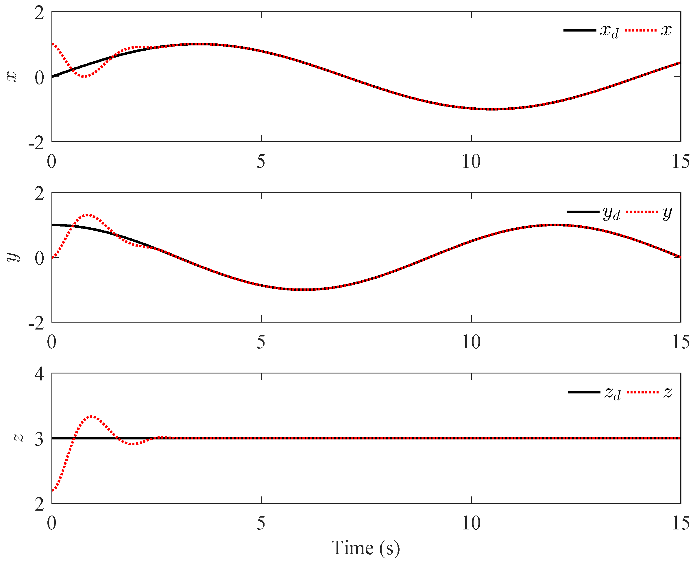
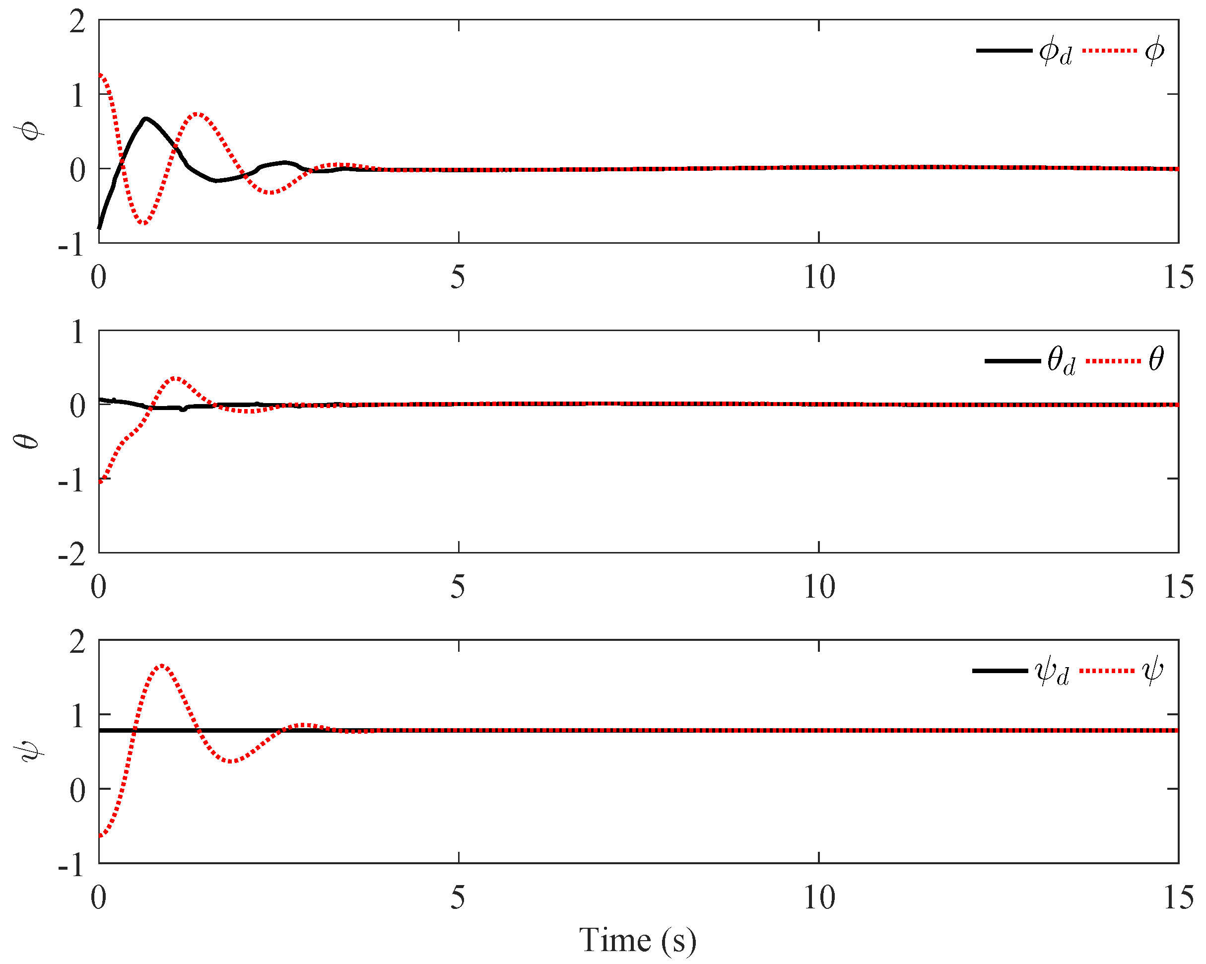
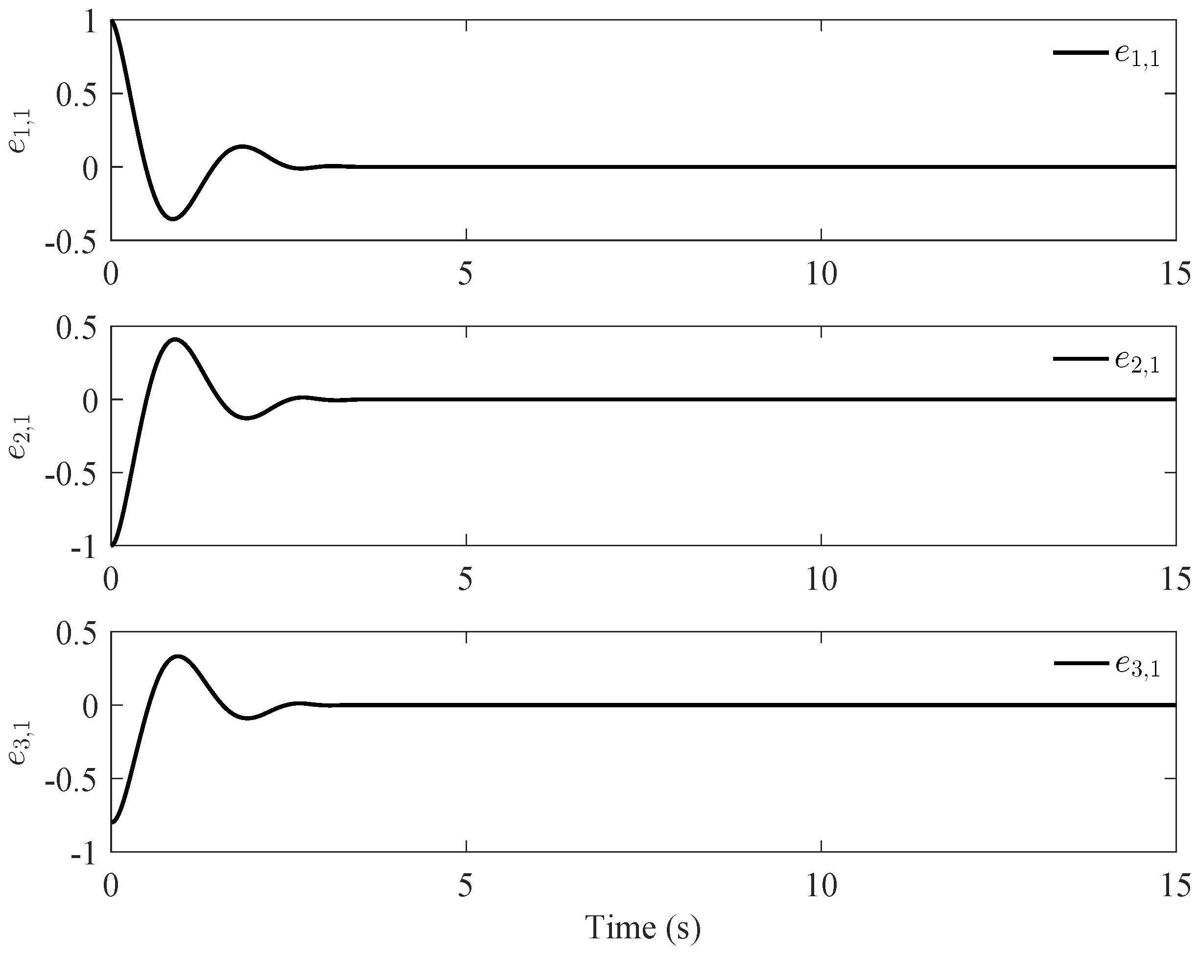
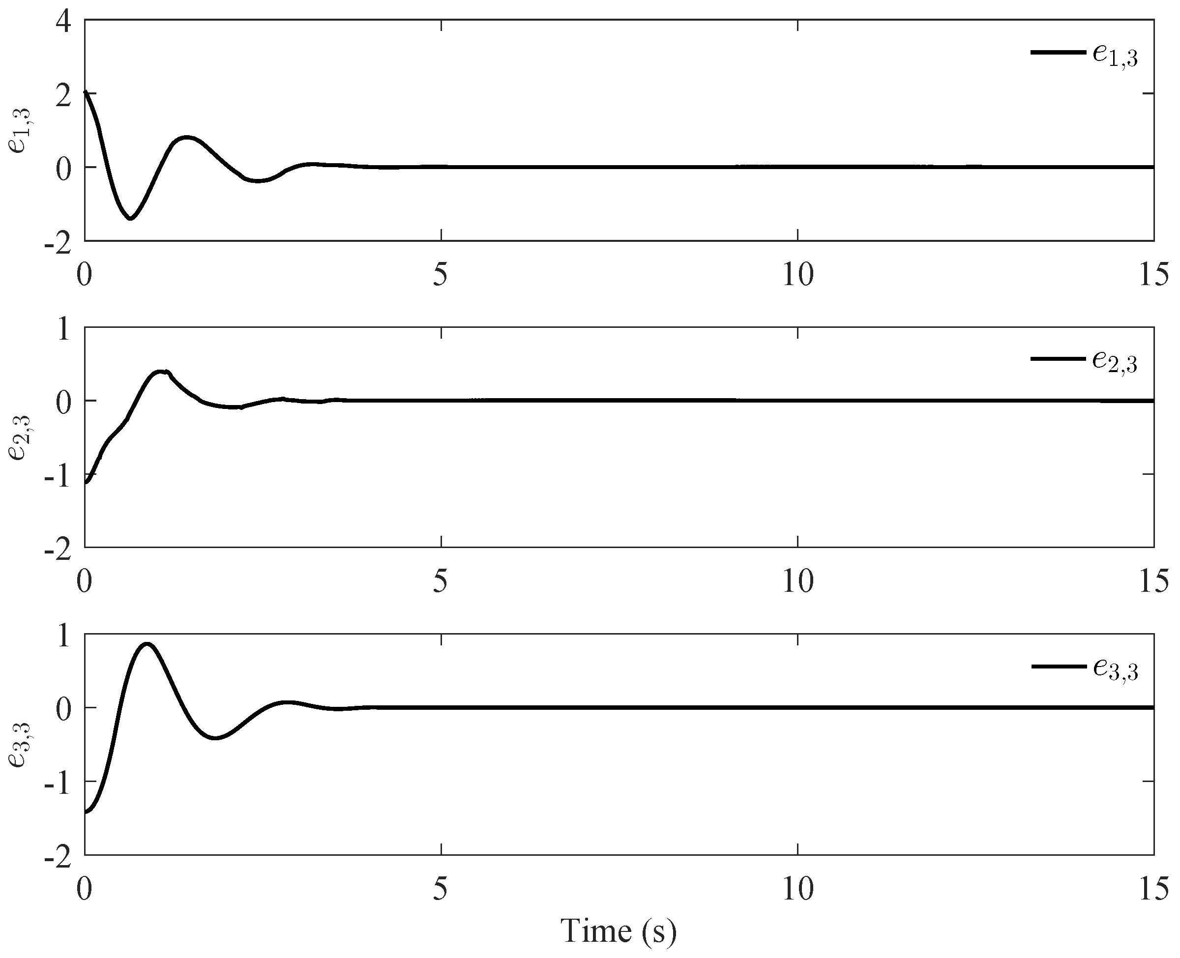
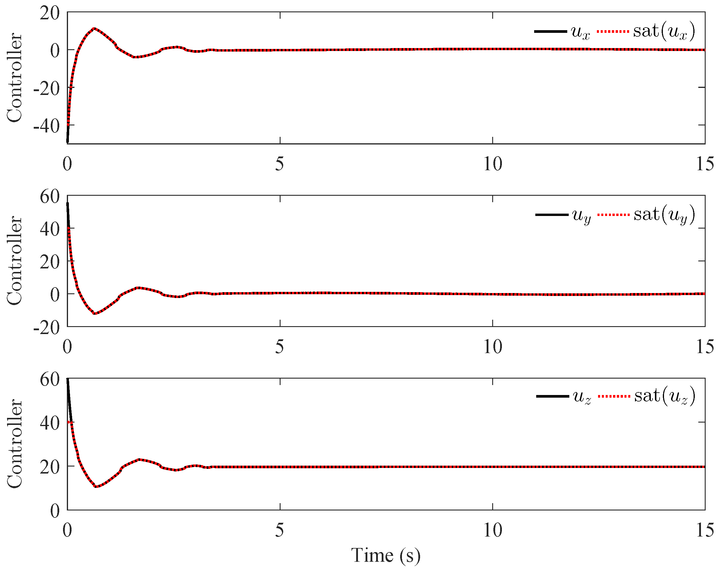
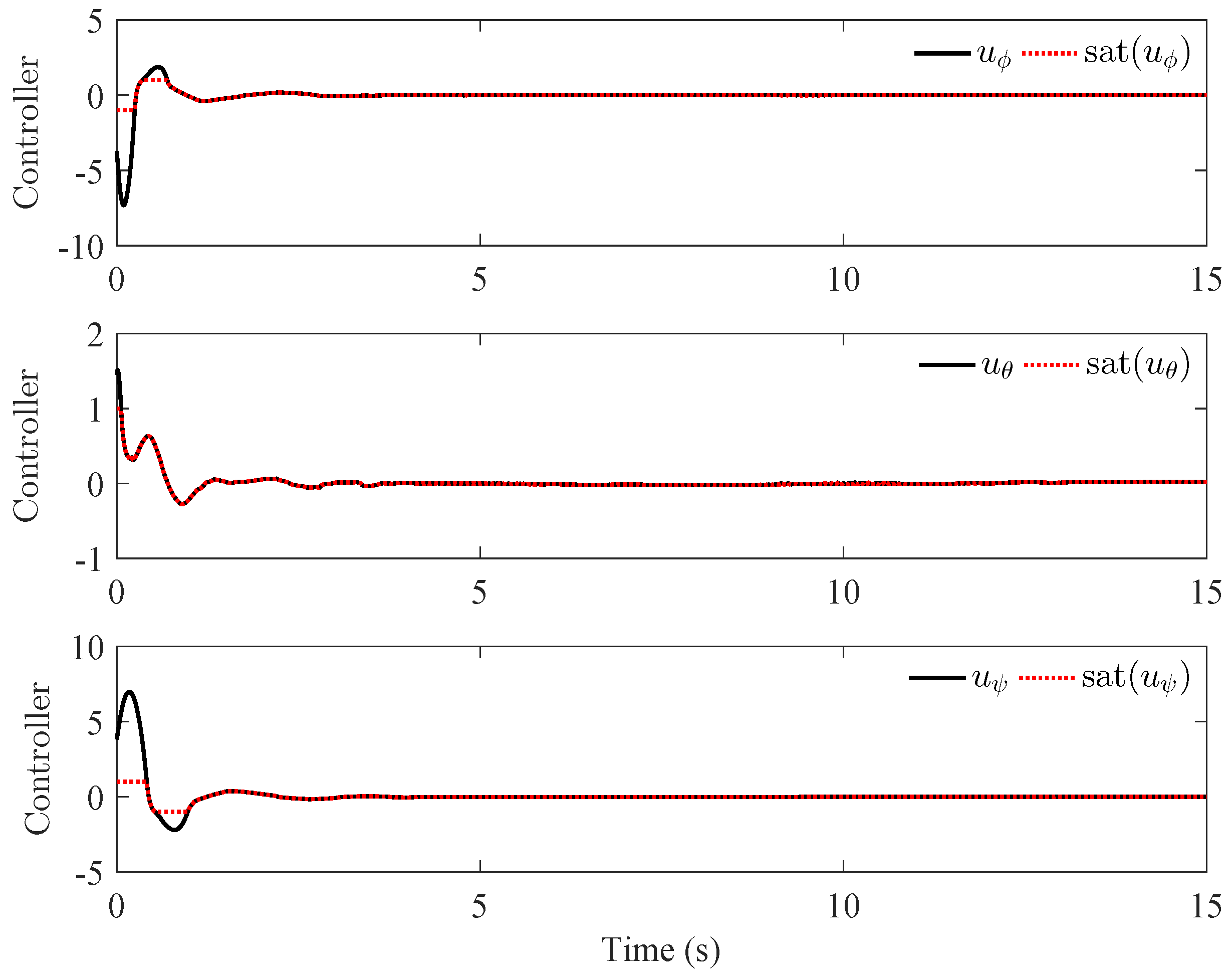
4. Simulation Results

By implementing a numerical simulation, the effectiveness of the developed fixed-time adaptive control scheme was demonstrated. The parameters of the QUAV are shown in Table 1.
The desired signals were set as x d = sin ( π t / 7 ) , y d = cos ( π t / 6 ) , z d = 3 , and ψ d = π / 4 . The external disturbances were assumed as d k = 0.01 sin ( π t / 10 ) , k = x , y , z , ϕ , θ , ψ . The initial states of the QUAV were chosen as [ x ( 0 ) , y ( 0 ) , z ( 0 ) , ϕ ( 0 ) , θ ( 0 ) , ψ ( 0 ) ] = [ 1 , 0 , 2.2 , 2 π 5 , π 3 , π 5 ] . The input saturations for QUAV were selected as [ Φ x , L , Φ y , L , Φ z , L , Φ ϕ , L , Φ θ , L , Φ ψ , L ] = [ 40 , 40 , 40 , 1 , 1 , 1 ] , and [ Φ x , R , Φ y , R , Φ z , R , Φ ϕ , R , Φ θ , R , Φ ψ , R ] = [ 40 , 40 , 40 , 1 , 1 , 1 ] . The control parameters were listed as a i , j = a ˘ i , j = 2.5 , b i , j = b ˘ i , j = 2 , m i , s = m ˘ i , s = 1.5 , Γ i , s = 1 , h i , s = 0.5 , R 1 = 2 , R 2 = 1 , μ = 1 , α = 5 / 7 , β = 7 / 5 , i = 1 , 2 , 3 , j = 1 , 2 , 3 , 4 , and s = 1 , 2 .
The simulation results are shown in Figure 2, Figure 3, Figure 4, Figure 5, Figure 6 and Figure 7. Figure 2 and Figure 3 display the trajectory tracking curves for the position and attitude subsystems of the QUAV. Figure 4 and Figure 5 describe the tracking errors of the position and attitude subsystems. Figure 6 and Figure 7 show the response curves of control inputs for the QUAV. Obviously, despite the QUAV being subject to input saturation, parameter uncertainties, and external disturbances, it can precisely and rapidly track the desired signals within 5 s. The tracking errors can converge to a sufficiently small region near the origin in a fixed time, and the control inputs do not violate the predefined constraints.
To show the superiority of the proposed fixed-time adaptive control scheme for the QUAV with input saturation, the command filtered backstepping (CFB) control scheme in [12] was utilized for a comparison. The control parameters for the CFB control scheme were chosen as a i , j = 0 , a ˘ i , j = 2.5 , b i , j = 0 , b ˘ i , j = 2 , m i , s = 0 , m ˘ i , s = 1.5 , Γ i , s = 1 , h i , s = 0.5 , α = 0 , β = 1 , i = 1 , 2 , 3 , j = 1 , 2 , 3 , 4 , and s = 1 , 2 . The simulations were implemented in MATLAB R2016a/Simulink on a 1.80 GHz Intel(R) Core(TM) i7-8565U computer operating on Windows 11, where the solver was selected as the ode 4 and the fixed-step size was set to 0.01 s. Define the overall tracking error OTE = | | [ e 1 , 1 , e 2 , 1 , e 3 , 1 , e 1 , 3 , e 2 , 3 , e 3 , 3 ] | | ; the root-mean-square error RMSE = w = 1 M ( e 1 , 1 ( w ) 2 + e 2 , 1 ( w ) 2 + e 3 , 1 ( w ) 2 + e 1 , 3 ( w ) 2 + e 2 , 3 ( w ) 2 + e 3 , 3 ( w ) 2 ) / M to compare the tracking performance, where w is the sample index, and M is the total number of samples.
The OTE values of the proposed control scheme and the CFB control strategy in [12] are presented in Figure 8. The convergence time and the RMSE in the performance comparison between the two control schemes are shown in Table 2, where we suppose that the convergence time is the time after which OTE 0.1 always holds. It can be seen that the convergence time and RMSE of the proposed control scheme are lower than those of the CFB control strategy in [12]. Clearly, when compared with the CFB in [12], the proposed fixed-time adaptive tracking control strategy not only has a quicker convergence rate, but also achieves better tracking performance.

5. Conclusions

This article has proposed a fixed-time adaptive tracking control scheme for a QUAV suffering from input saturation, parameter uncertainties, and external disturbances. By designing the fixed-time command filter and the fractional power-error compensation mechanism, the fixed-time command-filtered backstepping technique can tackle the problem of EOC and remove the influence of filtered error simultaneously. The auxiliary system with fixed-time convergence was constructed to compensate for the effect of input saturation. It proved that the tracking errors converge to a sufficiently small region near the origin in a fixed time. Simulation results have verified the effectiveness and superiority of the proposed fixed-time, adaptive control algorithm.

Author Contributions

Methodology, H.W. and G.C.; software, H.W.; writing—original draft preparation, H.W.; writing—review and editing, H.L. and G.C.; supervision, G.C. All authors have read and agreed to the published version of the manuscript.

Funding

This research was funded by the Natural Science Fund for Excellent Young Scholars of Jiangsu Province under Grant BK20211605; the National Natural Science Foundation of China under Grants 61703059 and 61873144; and the Post-graduate Research & Practice Innovation Program of Jiangsu Province under Grant SJCX21_1419.

Data Availability Statement

Not applicable.

Conflicts of Interest

The authors declare no conflict of interest.

Nomenclature

mMass
gGravitational acceleration
X = [ x , y , z ] Position
Θ = [ ϕ , θ , ψ ] Euler angles (roll, pitch, yaw)
ν = [ x ˙ , y ˙ , z ˙ ] Linear velocity
Ω = [ ϕ ˙ , θ ˙ , ψ ˙ ] Angular velocity
J = diag { J x , J y , J z } Inertia matrix
F X = diag { F x , F y , F z } Coefficients of resistance in position subsystem
F Θ = diag { F ϕ , F θ , F ψ } Coefficients of resistance in attitude subsystem
d X = [ d x , d y , d z ] External disturbance in position subsystem
d Θ = [ d ϕ , d θ , d ψ ] External disturbance in attitude subsystem
u F Total lift
U Θ = [ u ϕ , u θ , u ψ ] Control torque of attitude subsystem

References

  1. Choi, Y.C.; Ahn, H.S. Nonlinear control of quadrotor for point tracking: Actual implementation and experimental tests. IEEE/ASME Trans. Mechatron. 2015, 20, 1179–1192. [Google Scholar] [CrossRef]
  2. Yu, Y.; Ding, X. A global tracking controller for underactuated aerial vehicles: Design, analysis, and experimental tests on quadrotor. IEEE/ASME Trans. Mechatron. 2016, 21, 2499–2511. [Google Scholar] [CrossRef]
  3. Lu, Q.; Ren, B.; Parameswaran, S. Uncertainty and disturbance estimator-based global trajectory tracking control for a quadrotor. IEEE/ASME Trans. Mechatron. 2020, 25, 1519–1530. [Google Scholar] [CrossRef]
  4. Li, B.; Gong, W.; Yang, Y.; Xiao, B.; Ran, D. Appointed fixed time observer-based sliding mode control for a quadrotor UAV under external disturbances. IEEE Trans. Aerosp. Electron. Syst. 2021, 58, 290–303. [Google Scholar] [CrossRef]
  5. Wang, R.; Liu, J. Trajectory tracking control of a 6-DOF quadrotor UAV with input saturation via backstepping. J. Frankl. Inst. 2018, 355, 3288–3309. [Google Scholar] [CrossRef]
  6. Zhang, X.; Wang, Y.; Zhu, G. Compound adaptive fuzzy quantized control for quadrotor and its experimental verification. IEEE Trans. Cybern. 2021, 51, 1121–1133. [Google Scholar] [CrossRef]
  7. Xie, H.; Lynch, A.F.; Low, K.H.; Mao, S. Adaptive output-feedback image-based visual servoing for quadrotor unmanned aerial vehicles. IEEE Trans. Control Syst. Technol. 2020, 28, 1034–1041. [Google Scholar] [CrossRef]
  8. Shao, X.; Sun, G.; Yao, W.; Liu, J.; Wu, L. Adaptive sliding mode control for quadrotor UAVs with input saturation. IEEE/ASME Trans. Mechatron. 2021, 27, 1498–1509. [Google Scholar] [CrossRef]
  9. Koksal, N.; An, H.; Fidan, B. Backstepping-based adaptive control of a quadrotor UAV with guaranteed tracking performance. ISA Trans. 2020, 105, 98–110. [Google Scholar] [CrossRef]
  10. Shen, Z.; Li, F.; Cao, X.; Guo, C. Prescribed performance dynamic surface control for trajectory tracking of quadrotor UAV with uncertainties and input constraints. Int. J. Control 2021, 94, 2945–2955. [Google Scholar] [CrossRef]
  11. Farrell, J.A.; Polycarpou, M.; Sharma, M.; Dong, W. Command filtered backstepping. IEEE Trans. Autom. Control 2009, 54, 1391–1395. [Google Scholar] [CrossRef]
  12. Hu, C.; Zhang, Z.; Zhou, X.; Wang, N. Command filter-based fuzzy adaptive nonlinear sensor-fault tolerant control for a quadrotor unmanned aerial vehicle. Trans. Inst. Meas. Control 2020, 42, 198–213. [Google Scholar] [CrossRef]
  13. Aboudonia, A.; El-Badawy, A.; Rashad, R. Active anti-disturbance control of a quadrotor unmanned aerial vehicle using the command-filtering backstepping approach. Nonlinear Dyn. 2017, 90, 581–597. [Google Scholar] [CrossRef]
  14. Bhat, S.P.; Bernstein, D.S. Finite-time stability of continuous autonomous systems. SIAM J. Control Optim. 2000, 38, 751–766. [Google Scholar] [CrossRef]
  15. Liu, K.; Wang, X.; Wang, R.; Sun, G.; Wang, X. Antisaturation finite-time attitude tracking control based observer for a quadrotor. IEEE Trans. Circuits Syst. II Express Br. 2020, 68, 2047–2051. [Google Scholar] [CrossRef]
  16. Chen, Q.; Ye, Y.; Hu, Z.; Na, J.; Wang, S. Finite-time approximation-free attitude control of quadrotors: Theory and experiments. IEEE Trans. Aerosp. Electron. Syst. 2021, 57, 1780–1792. [Google Scholar] [CrossRef]
  17. Wang, F.; Gao, H.; Wang, K.; Zhou, C.; Zong, Q.; Hua, C. Disturbance observer-based finite-time control design for a quadrotor UAV with external disturbance. IEEE Trans. Aerosp. Electron. Syst. 2021, 57, 834–847. [Google Scholar] [CrossRef]
  18. Polyakov, A. Nonlinear feedback design for fixed-time stabilization of linear control systems. IEEE Trans. Autom. Control 2011, 57, 2106–2110. [Google Scholar] [CrossRef] [Green Version]
  19. Pan, Y.; Du, P.; Xue, H.; Lam, H.K. Singularity-free fixed-time fuzzy control for robotic systems with user-defined performance. IEEE Trans. Fuzzy Syst. 2021, 29, 2388–2398. [Google Scholar] [CrossRef]
  20. Gao, Z.; Guo, G. Command filtered finite/fixed-time heading tracking control of surface vehicles. IEEE/CAA J. Autom. Sin. 2021, 8, 1667–1676. [Google Scholar] [CrossRef]
  21. Du, H.; Zhang, J.; Wu, D.; Zhu, W.; Li, H.; Chu, Z. Fixed-time attitude stabilization for a rigid spacecraft. ISA Trans. 2020, 98, 263–270. [Google Scholar] [CrossRef]
  22. Shao, X.; Tian, B.; Yang, W. Fixed-time trajectory following for quadrotors via output feedback. ISA Trans. 2021, 110, 213–224. [Google Scholar] [CrossRef]
  23. Zhou, S.; Guo, K.; Yu, X.; Guo, L.; Xie, L. Fixed-time observer based safety control for a quadrotor UAV. IEEE Trans. Aerosp. Electron. Syst. 2021, 57, 2815–2825. [Google Scholar] [CrossRef]
  24. Cui, G.; Yang, W.; Yu, J.; Li, Z.; Tao, Z. Fixed-time prescribed performance adaptive trajectory tracking control for a QUAV. IEEE Trans. Circuits Syst. II Express Br. 2022, 69, 494–498. [Google Scholar] [CrossRef]
  25. Chen, Q.; Tao, M.; He, X.; Tao, L. Fuzzy adaptive nonsingular fixed-time attitude tracking control of quadrotor UAVs. IEEE Trans. Aerosp. Electron. Syst. 2021, 57, 2864–2877. [Google Scholar] [CrossRef]
  26. Wen, C.; Zhou, J.; Liu, Z.; Su, H. Robust adaptive control of uncertain nonlinear systems in the presence of input saturation and external disturbance. IEEE Trans. Autom. Control 2011, 56, 1672–1678. [Google Scholar] [CrossRef]
  27. Cui, G.; Xu, S.; Lewis, F.L.; Zhang, B.; Ma, Q. Distributed consensus tracking for non-linear multi-agent systems with input saturation: A command filtered backstepping approach. IET Control Theory Appl. 2016, 10, 509–516. [Google Scholar] [CrossRef]
  28. Mofid, O.; Mobayen, S. Adaptive finite-time backstepping global sliding mode tracker of quad-rotor UAVs under model uncertainty, wind perturbation, and input saturation. IEEE Trans. Aerosp. Electron. Syst. 2021, 58, 140–151. [Google Scholar] [CrossRef]
  29. Dun, A.; Wang, R.; Lei, F.; Yang, Y. Dynamic surface control for formation control of quadrotors with input constraints and disturbances. Trans. Inst. Meas. Control 2022, 44, 2500–2510. [Google Scholar] [CrossRef]
  30. Wang, L. Adaptive Fuzzy Systems and Control, Design and Stability Analysis; Prentice-Hall: Englewood Cliffs, NJ, USA, 1994. [Google Scholar]
  31. Qian, C.; Lin, W. A continuous feedback approach to global strong stabilization of nonlinear systems. IEEE Trans. Autom. Control 2001, 46, 1061–1079. [Google Scholar] [CrossRef]
  32. Yang, H.; Ye, D. Adaptive fixed-time bipartite tracking consensus control for unknown nonlinear multi-agent systems: An information classification mechanism. Inf. Sci. 2018, 459, 238–254. [Google Scholar] [CrossRef]
  33. Zuo, Z. Nonsingular fixed-time consensus tracking for second-order multi-agent networks. Automatica 2015, 54, 305–309. [Google Scholar] [CrossRef]
  34. Ba, D.; Li, Y.; Tong, S. Fixed-time adaptive neural tracking control for a class of uncertain nonstrict nonlinear systems. Neurocomputing 2019, 363, 273–280. [Google Scholar] [CrossRef]
  35. Cruz-Zavala, E.; Moreno, J.A.; Fridman, L.M. Uniform robust exact differentiator. IEEE Trans. Autom. Control 2011, 56, 2727–2733. [Google Scholar] [CrossRef]
Figure 1. The structure of the QUAV.
Actuators 12 00130 g001
Figure 2. The tracking curves of the position subsystem.
Actuators 12 00130 g002
Figure 3. The tracking curves of the attitude subsystem.
Actuators 12 00130 g003
Figure 4. The tracking errors of the position subsystem.
Actuators 12 00130 g004
Figure 5. The tracking errors of the attitude subsystem.
Actuators 12 00130 g005
Figure 6. The control inputs of the position subsystem.
Actuators 12 00130 g006
Figure 7. The control inputs of the attitude subsystem.
Actuators 12 00130 g007
Figure 8. The OTE under different control schemes.
Actuators 12 00130 g008
Table 1. The modeled parameters of the QUAV.
ParameterValueUnits
m2 kg
g9.8 m / s 2
J x , J y 0.045 kg · m 2
J z 0.083 kg · m 2
F x , F y , F z 0.01 kg / m
F ϕ , F θ , F ψ 0.01 kg / rad
Table 2. Performance comparison.
SchemeConvergence Time (s)RMSE
Proposed2.870.4922
CFB in [12]4.840.5354
Disclaimer/Publisher’s Note: The statements, opinions and data contained in all publications are solely those of the individual author(s) and contributor(s) and not of MDPI and/or the editor(s). MDPI and/or the editor(s) disclaim responsibility for any injury to people or property resulting from any ideas, methods, instructions or products referred to in the content.

