Analytical Derivation and Analysis of Vertical and Lateral Installation Ratios for Swing Axle, McPherson and Double Wishbone Suspension Architectures

Abstract

In the context of suspension design, the installation ratio (or motion ratio) is a parameter that relates wheel movement with spring deflection, quite an important kinematic property of a suspension. Yet, no study in the literature provides a clear relationship between the installation ratio and the geometrical features of a suspension. This paper employs rigid body kinematics and appropriate geometrical schematics to fill such a gap. Analytical expressions of the installation ratio are derived for three suspension layouts: swing axle, McPherson, double wishbone. Key concepts such as instant center, roll center and camber gain are harnessed to provide insightful analyses for relevant case studies of suspension passenger cars. Among the key results, the typical assumption of a McPherson installation ratio close to 1 is supported by a formal demonstration, and the new concept of “lateral” installation ratio is introduced which, alongside the classical “vertical” installation ratio, further characterizes suspension motion. Numerical results obtained through a multibody software support the findings of this paper. In conclusion, this study provides valuable insights for suspension design engineers.

1. Introduction

The suspension system is an essential feature of any passenger car, significantly contributing to comfort and safety. Many approaches to suspension design have been proposed over the years [1], with independent suspensions playing a major role.

Essentially, an independent suspension is a mechanism that provides the wheel assembly with a single degree of freedom (DOF) with respect to the vehicle chassis. Independent suspensions are designed to guarantee almost vertical (with respect to the road surface) motion of the wheel center. Steering wheels have an additional degree of freedom, allowing the wheel to spin around a quasi vertical axis. It is worth noting that many independent suspension schemes include a torsion bar, which elastically connects the wheels of the same axle. However this is not a kinematic connection and it is accepted that wheels can be still defined independent. In general, suspension design is a complex topic that has been widely investigated in the literature [2,3,4,5,6,7,8,9,10,11,12,13,14,15,16,17].

Within the many kinematic parameters at stake in suspension design, this paper focuses on the installation ratio (also known as motion ratio), defined as the ratio between spring deflection and wheel movement [1]. Based on this definition, the installation ratio relates wheel forces to spring forces. Ride natural frequency is one of the many variables affected by the installation ratio [18]. Interestingly, ref. [19] suggests: “If we were able to mount the spring directly over the centerline of the tire and we were able to mount it vertically, then the wheel rate would be equal to the spring rate (unitary installation ratio). We cannot achieve this due to packaging considerations”. This leads to think that it is impossible to have a unitary installation ratio. On the other hand, it is common knowledge that the McPherson suspension approximates this behavior pretty well. For instance, [20] declares “For MacPherson Strut suspension system the Motion Ratio remains to be 1:1”. However, to the best of the authors’ knowledge, a formal demonstration of this is missing in the literature.

Another typical suspension architecture is the double wishbone layout [21]. Also for this architecture, it is difficult to retrieve details on the installation ratio. For instance, ref. [22] proposes a very detailed analysis of the kinematic properties of double wishbone and McPherson architectures, but no reference is made to installation ratio. Many other contributions, e.g., [8,9,10,11,12,13,14,15,16,17], use the installation ratio in their studies, yet a rigorous analysis showing the dependence of the installation ratio on the suspension design parameters is missing.

This paper presents, for the first time, the derivation of analytical expressions of the installation ratio as a function of geometrical parameters of the suspension. This is applied to the McPherson and double wishbone layouts, along with the simple swing axle suspension. Furthermore, the classical installation ratio is herein further specified as “vertical”, supporting the introduction of the new concept of “lateral” installation ratio.

Section 2 recaps the key features of the studied passenger car suspension schemes. Section 3 details the most relevant suspension kinematic features, including installation ratio and camber gain, and it introduces the concept of lateral installation ratio. Section 4 derives analytical expressions for the installation ratios of the suspension schemes seen in Section 2. Section 5 discusses the results and, based on the outcomes, presents and analyzes a further variation of the McPherson suspension layout. Conclusions are drawn in Section 6.

2. Suspension Layout/Architecture

Swing-axle, McPherson and double wishbone suspensions are typically represented through simplified planar schemes where all the joints are assumed ideal, not including any elastic or damping element, except for the shock absorber. Considering the vehicle reference frame represented in Figure 1, planar suspension schemes are commonly represented on $y-z$ plane.

Figure 2a shows a three-dimensional representation of a swing axle suspension, consisting of a rigid traversal arm, which in this paper is assumed to be parallel to the y-axis. The arm is connected to the vehicle chassis by a revolute joint aligned with the vehicle x-axis. The wheel upright is integrated or rigidly connected on the swing axle, while the shock absorber group (spring and damper) is connected to the wheel upright (or to the swing arm) and to the vehicle chassis using a spherical (ball) joint. Figure 2b shows the equivalent 2D scheme of the swing axle suspension, where the shock absorber is connected to the wheel upright and is oriented along the unit vector $\underline{\lambda }$, with angle $\psi$ with respect to the vertical.

This type of suspension is rather inexpensive, but has poor handling characteristics, mainly because the wheel instant center depends on the swing axle length, usually limited by layout constraints.

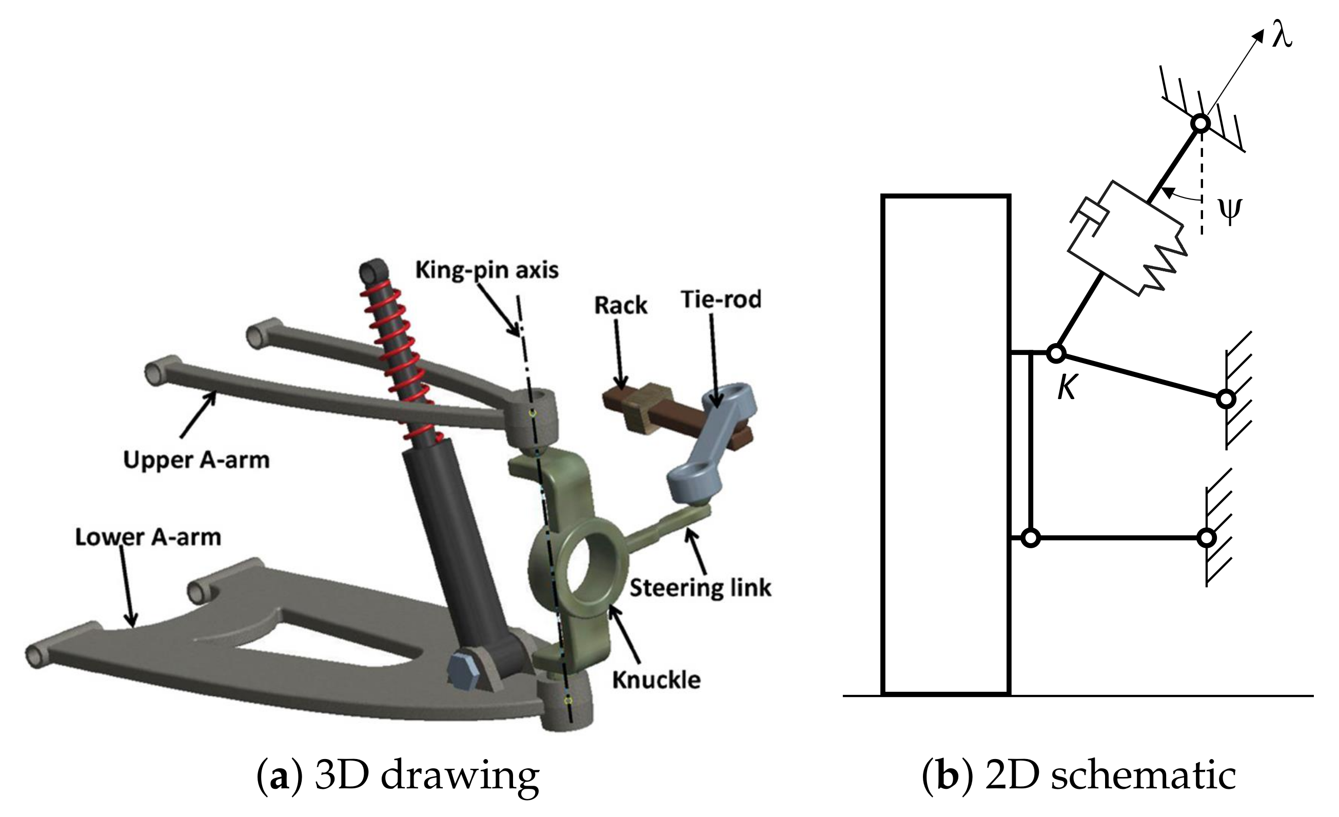
Figure 3a shows a three-dimensional representation of a McPherson suspension. A lower arm is connected to the vehicle chassis through a revolute joint, and to the upright through a ball joint. The upright is fixed to the strut, which includes the damper and that is kinematically represented by a cylindrical joint. The upper end of the strut is connected to the vehicle chassis by a ball joint. The upright is also connected with tie rod to the vehicle chassis or, in case of a steering wheel, to the steering box. Figure 3b shows the equivalent 2D scheme of the McPherson suspension, used to analyze the almost-vertical motion of the wheel. In order to reduce the scheme from 3D to 2D, the following assumptions are made:

• the tie rod is not represented;
• the revolute joint between the lower arm and the chassis is aligned with the x-axis;
• the strut belongs to the $y-z$ plane which includes the wheel center;
• the spring is assumed to be co-axial with the strut. This is not a classic choice, due to static load bearing reasons (see [23]), but is assumed for the sake of clearness.

This type of suspension is widely used on passenger cars front axles, since it is quite cheap, it guarantees appreciable handling characteristics and it leaves space for the engine due to its compactness in traversal direction.

Figure 4a shows a three-dimensional representation of a double wishbone suspension, also called short-long arm suspension or A-arm suspension. This suspension is made up of two A-arms, each-one connected to the vehicle chassis through a revolute joint and to the wheel upright through a ball joint. As for the McPherson suspension, a tie rod, having ball joints at its ends, connects the wheel to the chassis. The shock absorber, also installed with two ball joints at its ends, connects an A-arm or the wheel upright to the chassis. The equivalent 2D scheme, shown in Figure 4b, is obtained under the following hypotheses:

• the tie rod is not represented;
• the revolute joints between the A-arms and the chassis are aligned with the x-axis;
• the shock absorber belongs to the $y-z$ plane which includes the wheel center.

This type of suspension is widely used in racing cars due to its simplicity and lightweight, and to the good handling and set-up characteristics.

In addition, the lower arm of each suspension is assumed to be aligned along the y-axis, unless otherwise specified.

3. Relevant Parameters for Suspension Analysis

In kinematic and static planar analysis of a suspension, two relevant parameters are considered for almost all the suspension architectures: the instant center and the installation ratio.

The instant center, identified as Point C, also called centro [1], is defined as the point, belonging to a body in planar motion, which has instantaneously zero velocity. This point, in general, does not coincide with a material point of the analyzed body. Given this definition, it is common to consider, instantaneously, the motion of the body as a rotation around this point.

The position of the instant center of rotation is related to the camber gain of the suspension. Considering an infinitesimal vertical displacement of the wheel center (or of the contact patch) $\mathrm{d}z$ and considering that the wheel assembly instantaneously rotates around C, it is possible to relate the camber variation of the wheel assembly $\mathrm{d}\gamma$ to $\mathrm{d}z$, as follows

$$\mathrm{d}\gamma =-arctan\left(\frac{\mathrm{d}z}{y_1+y_2}\right)$$

(1)

If Equation (1) is linearized, the camber gain ${\gamma }_Z$ is obtained as

$${\gamma }_Z=\frac{\mathrm{d}\gamma }{\mathrm{d}z}=-\frac{1}{y_1+y_2}$$

(2)

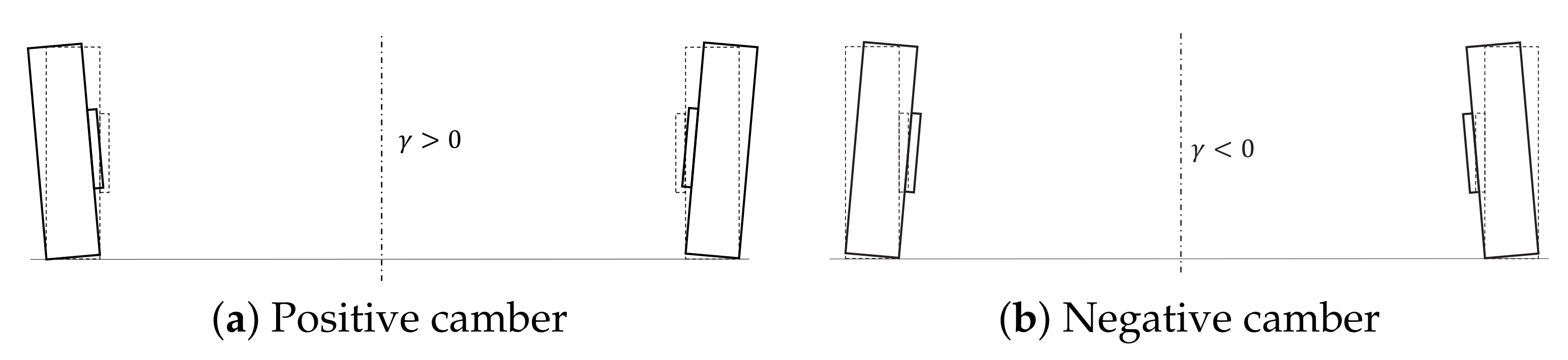
It is worth remarking that the camber angle sign is defined considering the symmetry property of the wheels, i.e., positive if oriented as shown in Figure 5a and negative as in Figure 5b.

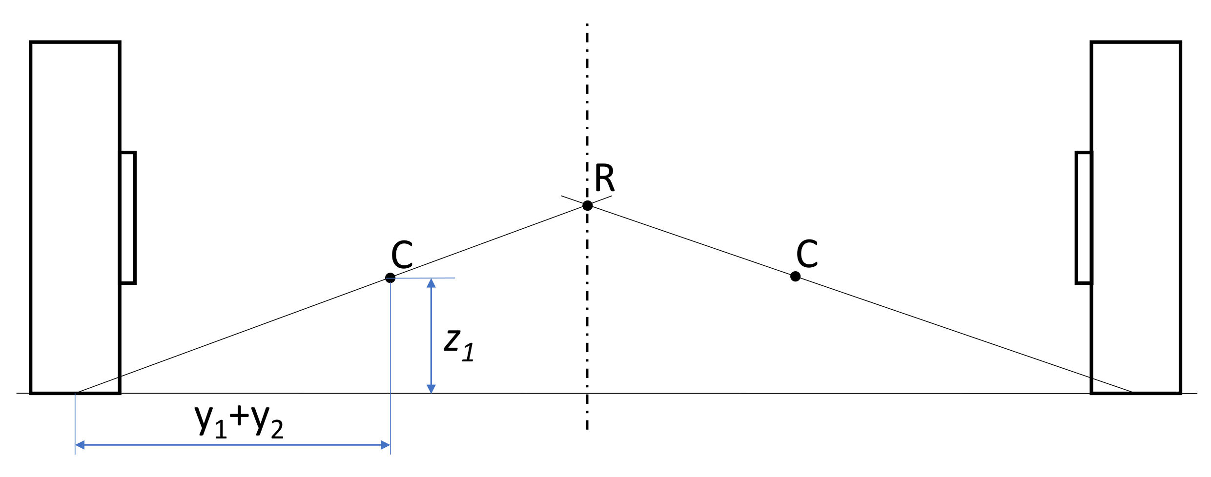
Often in the literature attention is devoted to the roll center R. Actually it can be obtained starting from the knowledge of the instant center. Indeed, as shown in Figure 6, the roll center is identified by the intersection of the line passing through the center of the contact patch and the instant center of rotation with the vertical symmetry plane of the vehicle.

The installation ratio, also called motion ratio [1], is introduced in order to relate the displacement, force and stiffness of the spring used in a suspension with the displacement, force and stiffness of an equivalent spring applied at the wheel center. It is worth noting that in this paper the spring and the translational joint introduced by the damper are assumed co-axial. This assumption allows to easily compute the installation ratio, assuming it to be the same for the spring and the damper. Actually, real suspension may not have exactly co-axial spring and damper, but a first guess of the installation ratio value is important for a preliminary design of the system. Further and more precise analyses can then be computed using multibody software.

Using the virtual work principle [24], the installation ratio is easily defined for a generic body. Consider a rigid body subject to forces $\underline{F_1}$ and $\underline{F_2}$ applied at two different locations of the body, A and B respectively (Figure 7). The equilibrium of the body is obtained solving Equation (3)

$$\underline{F_1}·\delta \underline{x_1}-\underline{F_2}·\delta \underline{x_2}=0$$

(3)

where $\delta \underline{x_1}$ and $\delta \underline{x_2}$ are the virtual displacements of point A and B, respectively. Assume $\delta x_{1,F}$ and $\delta x_{2,F}$ as the virtual displacement components aligned with each force. The equilibrium is obtained in scalar form as follows:

$$F_1\delta x_{1,F}-F_2\delta x_{2,F}=0$$

(4)

the installation ratio is then defined as

$$I=\frac{F_1}{F_2}=\frac{\delta x_{2,F}}{\delta x_{1,F}}$$

(5)

An equivalent form is obtained also if the velocity of point A and B are considered [1]: replacing the virtual displacements $\delta x_1$ and $\delta x_2$ with infinitesimal displacements $d{x}_1$ and $d{x}_2$ and dividing them by the infinitesimal time increment $dt$, Equation (5) becomes

$$I=\frac{F_1}{F_2}=\frac{v_{2,F}}{v_{1,F}}$$

(6)

where $v_{1,F}$ and $v_{2,F}$ are, respectively, the component of velocity of point A aligned with $\underline{F_1}$ and the component of velocity of point B aligned with $\underline{F_2}$. This analysis can be extended to multibody rigid systems, removing the hypothesis that A and B belong to the same rigid body.

In vehicles: (i) point A usually corresponds to the wheel contact patch center (or to the wheel center) and point B corresponds to the shock absorber end connected with the suspension; (ii) $\underline{F_1}$ and $\underline{F_2}$ are the vertical force at the ground ($F_z$) and the shock absorber force ($F_s$) respectively; (iii) $v_1$ is the velocity of the contact patch (or wheel center) along the vertical direction ($v_z$), and $v_2$ is the velocity of the shock absorber end connected to the suspension along the shock absorber axis ($v_s$). Hence, the (classical) vertical installation ratio, $I_Z$, considered if a vertical force is applied at the wheel center, is:

$$I_Z=\frac{F_z}{F_s}=\frac{v_s}{v_z}$$

(7)

An additional definition of installation ratio is proposed in this paper, which relates the force and displacement of the shock absorber with the lateral force $F_y$ and lateral velocity $v_y$ at the wheel contact patch center. Similarly to Equation (7), the lateral installation ratio $I_Y$ is defined as

$$I_Y=\frac{F_y}{F_s}=\frac{v_s}{v_y}$$

(8)

This parameter is not usually considered in the literature, but it has an important role on the suspension behavior. Indeed, when a lateral force is applied at the wheel center (i.e., during bending), the shock absorber force and displacement are influenced by the lateral force, causing a further compression or elongation of the shock absorber, in addition to the one due to the vertical load at the contact patch. As a result, the sprung mass vertical position changes also due to lateral force (i.e., jacking) and this phenomenon has to be considered also for choosing the shock absorber stroke.

4. Instant Centers and Analytical Derivation of Installation Ratios

For each of the suspension architectures investigated in this paper, in this section: (i) the position of the instant center, C, is analyzed; (ii) analytical expressions are obtained for vertical and lateral installation ratios, i.e., $I_Z$ and $I_Y$.

The reference frame $x_s$-$y_s$-$z_s$ used in each suspension scheme is centered in each suspension instant center (C) and has axes parallel to the general reference frame shown in Figure 1. Correspondingly, unit vectors $\underline{i}$, $\underline{j}$ and $\underline{k}$ identify the directions of, respectively, $x_s$, $y_s$ and $z_s$. Finally, the unit vector $\underline{\lambda }$ denotes the direction of the spring-damper system.

4.1. Swing Axle

As shown in Figure 8, the instant center C is physically determined by the hinge at the end of the suspension arm. Clearly, its position is independent of the inclination angle of the shock absorber, $\psi$.

Based on the definition given in Section 3, the vertical installation ratio is:

$$I_Z=\frac{\underline{v_K}·\underline{\lambda }}{\underline{v_P}·\underline{k}}$$

(9)

and the lateral installation ratio is:

$$I_Y=\frac{\underline{v_K}·\underline{\lambda }}{\underline{v_P}·\underline{j}}$$

(10)

where K and P are points on the upright, corresponding respectively to the top spherical joint (connecting the upright to the spring-damper system) and to the middle of the contact patch, and $\underline{v_K}$ and $\underline{v_P}$ are their velocities. These points are shown in Figure 8, which also indicates the position of the (physical) instant center of the mechanism, C. Following from the definition of instant center:

$$\begin{array}{c}\hfill \underline{v_P}=\omega \underline{i}\times \underline{CP}\end{array}$$

(11)

$$\begin{array}{c}\hfill \underline{v_K}=\omega \underline{i}\times \underline{CK}\end{array}$$

(12)

with (Figure 8)

$$\begin{array}{c}\hfill \underline{CP}=-(y_1+y_2)\underline{j}-z_1\underline{k}\end{array}$$

(13)

$$\begin{array}{c}\hfill \underline{CK}=-y_3\underline{j}+z_3\underline{k}\end{array}$$

(14)

and with $\omega$ being the angular velocity of the upright.

By using Equation (13) in Equation (11), Equation (14) in Equation (12), substituting in Equations (9) and (10):

$$I_Z=\frac{y_{3}cos\psi +z_{3}sin\psi }{y_1+y_2}$$

(15)

$$I_Y=-\frac{y_{3}cos\psi +z_{3}sin\psi }{z_1}$$

(16)

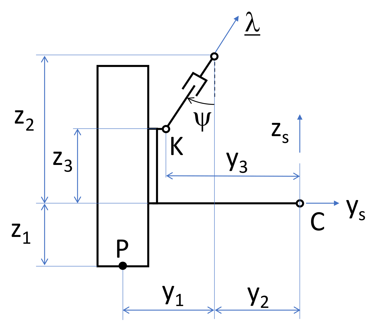
4.2. McPherson

In a McPherson architecture (Figure 9), the instant center C is said to be a virtual point because it is not longer a physical point (as it was the case for the swing axle). Through analytical mechanics [25] it is easy to show that C is the intersection between the lower control arm and a line perpendicular to the direction of the shock absorber. Clearly, the position of C depends on $\psi$.

Again based on the definition given earlier, the vertical installation ratio is:

$$I_Z=\frac{\underline{v_D}·\underline{\lambda }}{\underline{v_P}·\underline{k}}$$

(17)

and the lateral installation ratio is:

$$I_Y=\frac{\underline{v_D}·\underline{\lambda }}{\underline{v_P}·\underline{j}}$$

(18)

where D is a virtual point on the upright corresponding to the top spherical joint (connecting the spring-damper system to the vehicle chassis), and $\underline{v_D}$ is its velocity. Point D is shown in Figure 9, also indicating the position of the (virtual) instant center of the mechanism, C. Following from the definition of instant center:

$$\begin{array}{c}\hfill \underline{v_P}=\omega \underline{i}\times \underline{CP}\end{array}$$

(19)

$$\begin{array}{c}\hfill \underline{v_D}=\omega \underline{i}\times \underline{CD}\end{array}$$

(20)

with (Figure 9)

$$\begin{array}{c}\hfill \underline{CP}=-(y_1+y_2)\underline{j}-z_1\underline{k}\end{array}$$

(21)

$$\begin{array}{c}\hfill \underline{CD}=-y_2\underline{j}+z_2\underline{k}\end{array}$$

(22)

and with $\omega$ being the angular velocity of the upright.

By using Equation (21) in Equation (19), Equation (22) in Equation (20), substituting in Equations (17) and (18), and considering that $tan\psi =z_2/y_2$:

$$I_Z=\frac{1}{cos\psi +\frac{y_1}{z_2}sin\psi }$$

(23)

$$I_Y=-\frac{z_2}{z_{1}sin\psi }$$

(24)

4.3. Double Wishbone

As shown in Figure 10, for a double wishbone architecture the position of the instant center C is defined by the inclination of the upper wishbone, $\varphi$. Unlike the McPherson suspension, $\varphi$ and $\psi$ are independent, while C is still a virtual point.

Once again based on the definition given earlier, the vertical installation ratio is:

$$I_Z=\frac{\underline{v_K}·\underline{\lambda }}{\underline{v_P}·\underline{k}}$$

(25)

and the lateral installation ratio is:

$$I_Y=\frac{\underline{v_K}·\underline{\lambda }}{\underline{v_P}·\underline{j}}$$

(26)

where K is the point connecting upright and upper wishbone, and $\underline{v_K}$ is its velocity. Again, from the definition of instant center:

$$\begin{array}{c}\hfill \underline{v_P}=\omega \underline{i}\times \underline{CP}\end{array}$$

(27)

$$\begin{array}{c}\hfill \underline{v_K}=\omega \underline{i}\times \underline{CK}\end{array}$$

(28)

with (Figure 10)

$$\begin{array}{c}\hfill \underline{CP}=-(y_1+y_2)\underline{j}-z_1\underline{k}\end{array}$$

(29)

$$\begin{array}{c}\hfill \underline{CK}=-(y_2+y_3-y_4)\underline{j}+z_3\underline{k}\end{array}$$

(30)

and with $\omega$ being the angular velocity of the upright.

By using Equation (29) in Equation (27), Equation (30) in Equation (28), substituting in Equations (25) and (26):

$$I_Z=\frac{(y_2+y_3-y_4)cos\psi +z_{3}sin\psi }{y_1+y_2}$$

(31)

$$I_Y=\frac{(y_2+y_3-y_4)cos\psi +z_{3}sin\psi }{-z_1}$$

(32)

which may be rearranged in the more compact form:

$$I_Z=\frac{z_3}{y_1+y_2}\left(\frac{cos\psi }{tan\varphi }+sin\psi \right)$$

(33)

$$I_Y=-\frac{z_3}{z_1}\left(\frac{cos\psi }{tan\varphi }+sin\psi \right)$$

(34)

5. Discussion

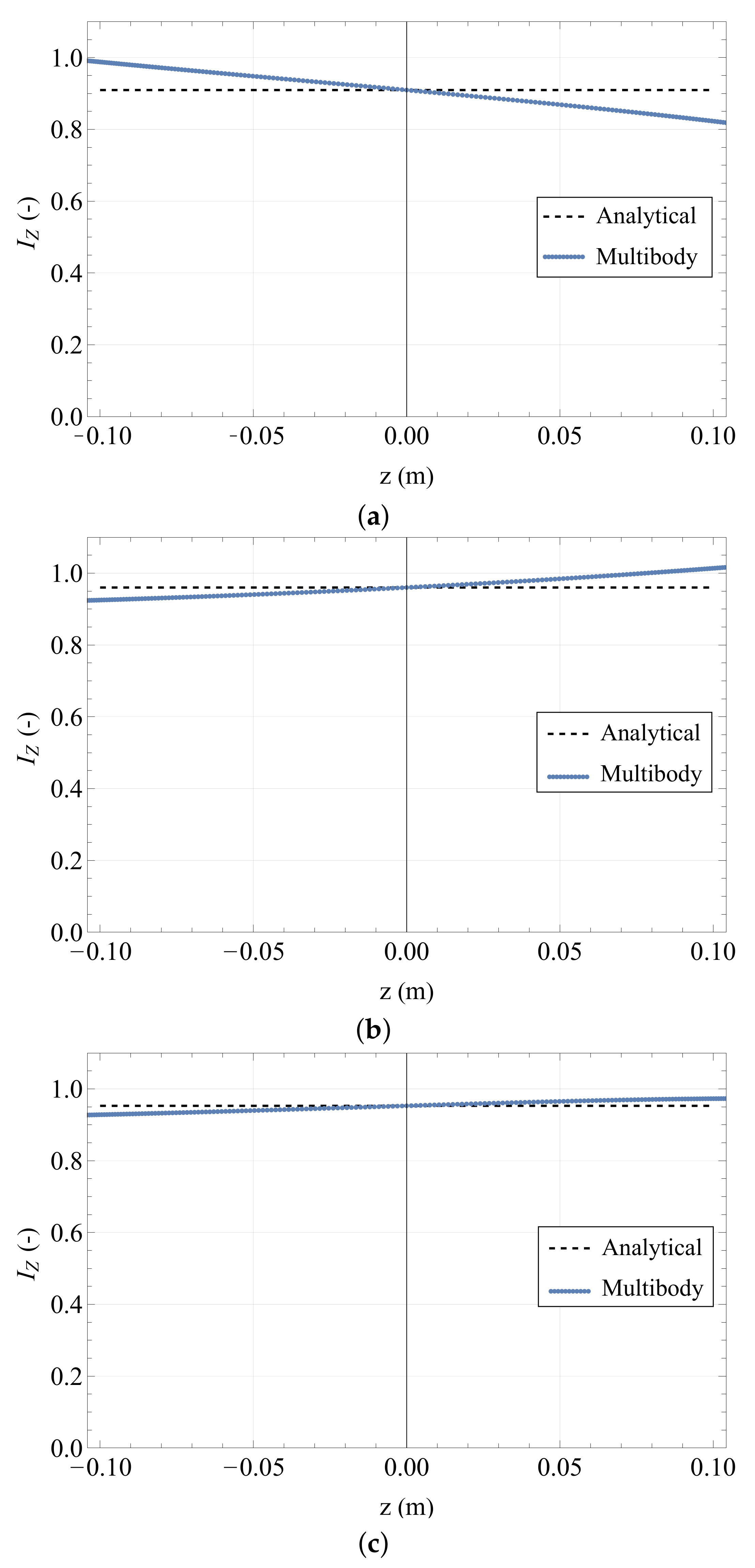
In light of the results of the previous section, a multibody (MB) model was developed in Adams View for each suspension architecture to validate the analytical results. Rigid bodies and ideal constraints were considered to reproduce, in the MB environment, the planar schemes shown in Figure 8, Figure 9 and Figure 10. The numerical values of the geometrical parameters used in this case study are listed in

Table 1. Geometrical parameters used for model validation.

Parameter	Swing Axle	McPherson	Double Whishbone
$\psi$	14${}^{\circ }$	14${}^{\circ }$	14${}^{\circ }$
$\varphi$	–	–	7.1${}^{\circ }$
$y_1$	0.25 m	0.25 m	0.25 m
$y_2$	0.35 m	0.35 m	1.85 m
$y_3$	0.50 m	0.50 m	0.50 m
$z_1$	0.15 m	0.15 m	0.15 m
$z_2$	0.85 m	0.85 m	0.85 m
$z_3$	0.50 m	0.25 m	0.25 m

.

A sinusoidal vertical motion (z) was imposed at wheel contact patch (point P) having $0.1$ m amplitude. The contact patch velocity, the shock absorber relative velocity and the wheel assembly rotation were measured. Figure 11 shows the comparison between the MB results and the analytical results for $I_Z$, obtained using Equations (15), (23) and (33).

The analytical formulae correctly estimate the vertical installation ratio for the reference configuration ($z=0$) for all the considered suspension schemes, while some differences appear as the suspension moves, because the analytical models assume infinitesimal displacement.

In the following subsections, further insights are given on the kinematic features of each suspension scheme. Physical interpretations of the expressions of installation ratios are given in the hypothesis of small spring-damper inclination, i.e., $\psi \ll 1$ rad (typical of a McPherson setup [1,26,27,28]). Such considerations are also related to the position of the instant center and the camber gain properties of each scheme.

5.1. Kinematic Features

Assuming $\psi \approx 0$, then $cos\psi \approx 1$ and $sin\psi \approx 0$. For the swing axle, Equation (15) reduces to:

$$I_Z=\frac{y_3}{y_1+y_2}$$

(35)

which can be easily interpreted: with the spring-damper being vertical, the vertical installation becomes the ratio between two vertical virtual displacements, i.e., the mere ratio between the horizontal distances between each point (K or P) and the instant center. Ideally, with points K and P vertically aligned, the vertical ratio would be 1. But since P is further apart from C than K, then the installation ratio Equation (35) ends up being less than 1. This is consistent the qualitative considerations seen in [19].

Similarly, Equation (16) reduces to:

$$I_Y=-\frac{y_3}{z_1}$$

(36)

Interestingly, for $z_1\Rightarrow 0$, $I_Y\Rightarrow \infty$, meaning that if P and C are horizontally aligned, P won’t move horizontally regardless of the movement of K (for little variations from the depicted configuration). Instead, if $y_3\Rightarrow 0$, $I_Y\Rightarrow 0$, meaning that if K and C are vertically aligned, then K will only move horizontally i.e., with a 0 component towards $\lambda$ (recall that $\lambda$ is vertical due to $\psi \approx 0$).

In terms of camber gain, from Equation (2) it is:

$${\gamma }_Z=-\frac{1}{y_1+y_2}$$

(37)

which is quite significant due to C being a physical point of the suspension. The large magnitude of the camber gain is a key drawback of the swing axle suspension. This issue is overcome in the McPherson and double wishbone architectures, since C is no longer a point belonging to the suspension assembly.

For the McPherson suspension with $\psi \approx 0$, Equation (23) reduces to:

$$I_Z=1$$

(38)

Since for a McPherson architecture $\psi \approx 0$ holds true due to layout constraints, Equations (23) and (38) formally prove the well-known fact that the vertical installation ratio of such a suspension is $\approx 1$. This is a key result of this paper.

Similarly, Equation (24) reduces to:

$$I_Y=\infty$$

(39)

Formally it would be a $\frac{0}{0}$ situation, because having $\psi \approx 0$ implies that C is at ∞ distance from the suspension. Thus, the whole suspension moves only due to vertical loads, while its motion is independent of lateral loads.

In terms of camber gain, from Equation (2) it is:

$${\gamma }_Z=-\frac{1}{y_1+y_2}$$

(40)

which is formally the same as Equation (37), but here $y_2$ can be way larger than for the swing axle, thus limiting the camber gain, again because C is virtual and $\psi$-dependent.

The double wishbone suspension, as discussed, has an additional degree of freedom, i.e., angle $\varphi$. It is interesting to see that if $\psi \approx 0$ and the upper and lower arms are parallel, then $y_2=\infty$ and Equation (31) reduces to:

$$I_Z=cos\psi \approx 1$$

(41)

while Equation (32) becomes:

$$I_Y=\infty$$

(42)

which corresponds to the situation seen above for the McPherson situation with $\psi \approx 0$. When it comes to camber gain, due to the instant center being virtual, the same considerations as for the McPherson suspension can be drawn.

5.2. McPherson Variation

A fundamental hypothesis introduced in Section 2 is related to the orientation of the lower arm (only one arm for the swing axle) of the suspension, which is assumed to be horizontal in the reference configuration. This assumption is related to layout issues, which usually force the lower arm to be almost horizontal in the reference configuration. However, if the lower arm is assumed to be inclined, a further design degree of freedom can be used by the suspension designer. This is appreciated especially for the McPherson suspension where, as discussed previously, the inclination of the spring-damper assembly $\psi$ and the position of the instant center C are not independent.

With reference to Figure 12, if the lower arm is inclined by an angle $\alpha$ with respect to the y-axis without modifying $\psi$, the instant center of rotation moves from C to $C^{\prime }$.

Consequently, the vertical installation ratio (Equation (23)) becomes

$$I_Z=\frac{1}{cos\psi +\frac{y_1}{z_2^{\prime }}sin\psi }$$

(43)

while the lateral installation ratio (Equation (24)) becomes

$$I_Y=-\frac{z_2^{\prime }}{y_{1}sin\psi }$$

(44)

and the camber gain becomes

$${\gamma }_Z=-\frac{1}{y_1+y_2^{\prime }}$$

(45)

where

$$y_2^{\prime }=y_2-\Delta y=y_2-\underline{C{C}^{\prime }}(\alpha ,\psi )cos\psi$$

(46)

and

$$z_2^{\prime }=z_2-\Delta z=z_2-\underline{C{C}^{\prime }}(\alpha ,\psi )sin\psi$$

(47)

and $\underline{C{C}^{\prime }}(\alpha ,\psi )$ can be obtained analytically.

In order to appreciate the influence of $\alpha$ on the vertical and lateral installation ratio and on the camber gain, a sensitivity analysis is proposed, keeping all the other suspension parameters unchanged. The constant suspension parameters are listed in

Table 2. Suspension parameters.

Parameter	Value
$\psi$	20${}^{\circ }$
$y_1$	0.3 m
$z_1$	0.3 m
$z_2$	0.8 m
$y_2$	$z_2$/$tan\psi$
$y_E$	$y_2$ + 0.1 m

.

Figure 13 shows the variation of the vertical (Figure 13a) and lateral (Figure 13b) installation ratios and of the camber gain (Figure 13c) with respect to the inclination of the lower arm $\alpha$. Figure 14 shows the percentage variation of the above parameters. With reference to the analyzed case study, whose parameters are inspired by real suspension architectures, it is worth pointing out that varying the lower arm inclination mainly affects the lateral installation ratio and the camber gain, whose percentage variation is about −75% and 200% for the considered range of $\alpha$, while the influence on the vertical installation ratio is lower (−28%). Hence, even if a general conclusion cannot be drawn by the single case study, it is confirmed that changing the inclination of the lower arm in a McPherson suspension allows to non-proportionally change the vertical installation ratio and the camber gain. For this reason, the suspension designer can vary both the strut inclination $\psi$ and the lower arm inclination $\alpha$ to obtain the desired value of the relevant parameters of the suspension. Even if they are not decoupled, their value can be optimized acting on two parameters instead of one.

6. Conclusions

Suspension mechanisms are usually studied by complex multibody models which allow to compute all the suspension characteristics. However, a simplified fundamental approach is useful to understand the most relevant parameters affecting suspension motion. Within this context, the installation ratio and the camber gain have been derived in this paper, considering 2D schemes, with reference to three suspension mechanisms: swing axle, McPherson and double wishbone. A novel concept is also introduced, i.e., the lateral installation ratio, which relates the suspension displacement with the lateral loads acting at the tire contact patch.

For each mechanism, the analytical formulation of these relevant parameters is computed as a function of the design variables. Considering the swing axle, the camber gain and the vertical installation ratio are independent, but the position of the instant center of rotation is related to the physical position of the revolute joint between the suspension and the chassis, limiting the designer’s freedom. Considering the McPherson suspension with horizontal lower arm, the installation ratio and the camber gain are mutually related, even if the instant center of rotation is a virtual point. Notably, we demonstrated that the vertical installation ratio of the McPherson suspension is close to 1. Considering the double wishbone suspension, the installation ratio and the camber gain are independent and the instant center of rotation is a virtual point. So, this is the suspension allowing the most design freedom. Interestingly, also the McPherson suspension allows a wider design freedom if the lower arm can be assumed not horizontal.

In terms of the designer’s perspective, the availability of analytical relationships for the installation ratios represents a further instrument in the engineer’s toolbox. He/she has insight on how changing one hardpoint, rather than another, affects the installation ratio along with other relevant quantities (e.g., camber gain, roll steer, etc.), thus optimizing the design process.