Article

Communication-Based Train Control with Dynamic Headway Based on Trajectory Prediction

1
National Engineering Research Center of Rail Transportation Operation and Control System, Beijing Jiaotong University, Beijing 100044, China
2
State Key Lab of Rail Traffic Control & Safety, Beijing Jiaotong University, Beijing 100044, China
*
Author to whom correspondence should be addressed.
Actuators 2022, 11(8), 237; https://doi.org/10.3390/act11080237
Submission received: 4 July 2022 / Revised: 9 August 2022 / Accepted: 15 August 2022 / Published: 18 August 2022

Abstract

:
Rail transit plays a significant role in the operation of an efficient and effective urban public transportation system. Safety and capacity are some of the most crucial objectives in railway operations. The communication-based train control (CBTC) system is a continuous and automatic train control system that realizes constant and high-capacity train ground two-way communication. In this study, a dynamic headway model of the ‘softwall’ moving-block approach is proposed for CBTC to increase the track capacity and improve dispatching efficiency based on the train trajectory prediction. For this precise trajectory prediction task, we introduce a hybrid trajectory prediction model to combine Long Short-term memory (LSTM) and Kalman Filter (KF) to extract the train’s local data features and learn the long-term dependencies, respectively. Then we present a dynamic headway model to maximize the train headway and reduce the track distance. The leading trains’ information is used to construct the iterative learning control strategy, and the predicted trajectory is input into the algorithm of the headway model. We use a simulation model of the rail network in Chengdu to demonstrate the effectiveness of our proposed approach. The results show the Mean Absolute Error (MAE) of the predicted trajectory retreated to 93.97 cm and reductions in operation headway of at least 64.33% under the dynamic headway model versus the traditional moving-block model.

1. Introduction

The urban railway has been developed in recent decades with outstanding achievements worldwide. However, the existing operating capacity has dramatically hindered the transportation efficiency and development of urban rail transit. The limited operating capacity has led to traffic congestion, especially during the peak hours of the metropolis. The increasing demand for railway transportation has brought tremendous pressure to the existing railway transportation system, which is expected to alleviate frequent traffic jams. Efficiency implies shorter travel times, higher track capacity, and reduced congestion delays.
The two primary ways to improve the efficiency of railway transportation are to increase the speed and the operation density, while the train operation speed has encountered a bottleneck. The minimum track headway, the optimum distance that the next train can achieve while following the lead train, is considered one of the major factors restricting operational capability.
Therefore, transportation efficiency can be improved by increasing the operation density under the condition of the original railway network, which is achieved by shortening the tracking interval of the train.
The two-way communication technology with a more significant amount of information transmission and fast transmission speed enables the increase of CBTC from a fixed-block system to a moving-block system. As shown in Figure 1, the CBTC is a “moving-block” signaling system, which is based on the “concrete wall” principle, and trains are allowed to be separated by an absolute-braking distance (where it is assumed that a massive rock falls in front of the leading train). However, as the trajectory prediction is only determined by the absolute position of the front train, in order to guarantee safety, the minimum train separation is decided by the absolute-braking distance, which limits the improvement of the traffic density.
Active communications in the CBTC system cause frequent information exchange between the control center and trains, including train dynamics and characteristics. This detailed information can lead to more modest but safe progress, considering train operation, speed, deceleration capabilities, etc. Therefore, we introduce trajectory prediction into the soft wall mode, enabling the more advanced calculation that considers that the leading train is running instead of stationary in the hard wall mode [1].
Most trajectory prediction research focuses on pedestrians, aircraft, automobiles, and other fields, but the train is a sizeable inertial body and cannot stop as quickly as it detects danger. Moreover, the CBTC system is designed to be unable to release once emergency braking is applied under safety considerations, and we should avoid these situations as much as possible. Hence, one crucial task of our approach is to predict the accurate and long-term trajectories of the train, which covers the emergency braking time window of the following train to achieve safe and robust driving.
Another task is to design a dynamic headway system for CBTC based on the predicted trajectory. It uses the future information to calculate its optimal safe distance relative to the lead train. Since such a headway is constantly updated, it is considered a dynamic headway. The dynamic track approach should also consider possible communication disruptions due to inclement weather or other failures and return gracefully and safely to a more conservative track without putting any trains at risk [2]. The distinct features of the proposed system are:
(1)
The trajectory prediction part can accurately predict the leading train’s trajectory over the following one’s emergency braking time.
(2)
A dynamic headway policy based on vehicle-to-vehicle and vehicle-to-center communications results in much smaller distances than existing ones based on fixed-block and moving-block policies.
(3)
A backup switching policy increases gracefully to the new situation without sacrificing security, such as lost communications.
In summary, the main contributions of this work are as follows:
1.
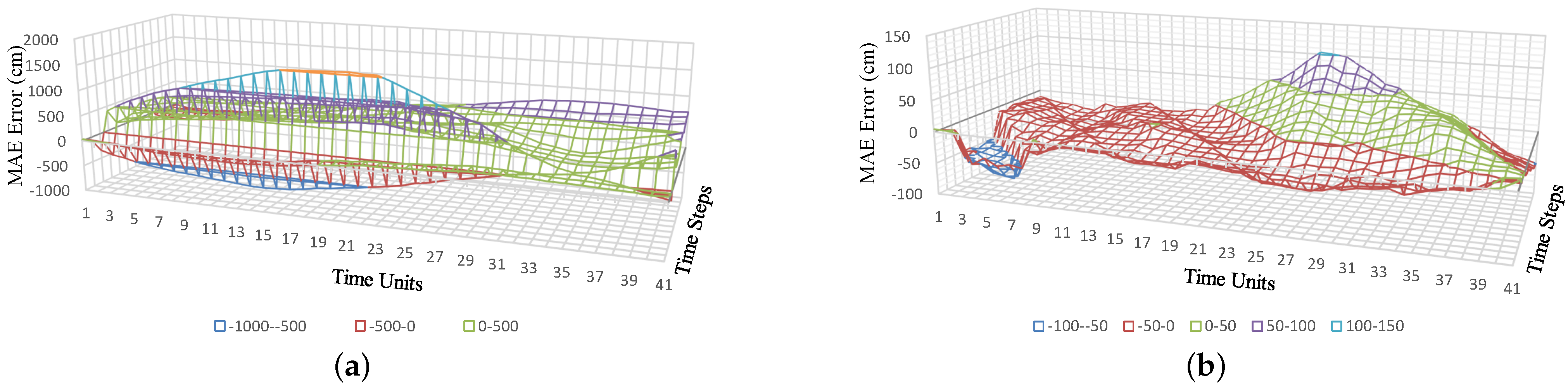
Aiming at the trajectory prediction problem for trains, a data-processing method and a hybrid prediction model which enable an accurate prediction even when the horizons are increased to 15 s is established for the first time.
2.
We used the concept of trajectory prediction and moving block and developed a soft wall control system that substantially reduces the distance between trains
3.
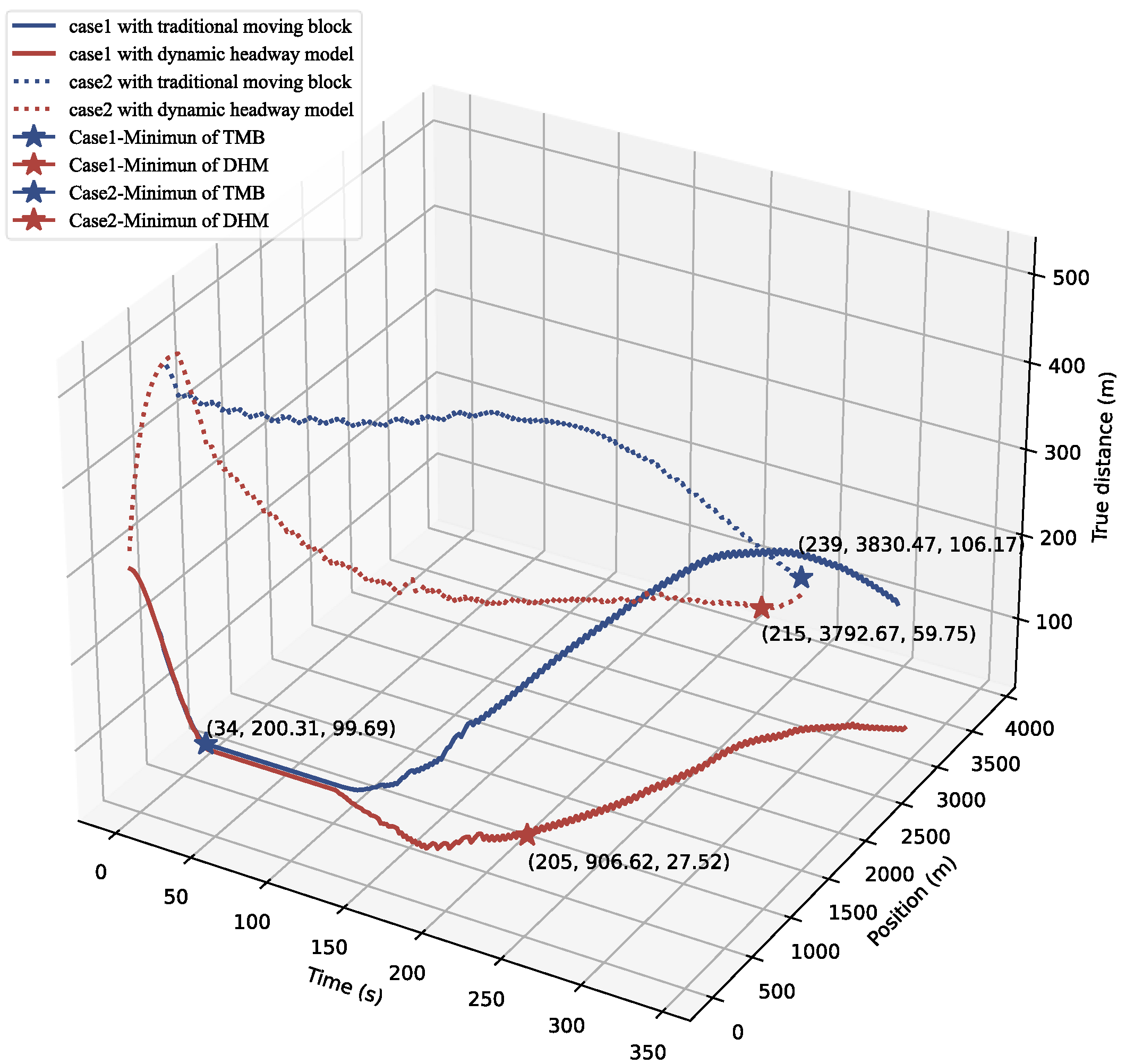
In contrast to the traditional moving block, our proposed dynamic headway system shows reductions in train headway of at least 64%.
The remainder of this paper is structured as follows. Section 2 summarizes the research of headway policy and trajectory prediction in deep learning and the dynamic headway compared with these headway policies. Section 3 introduces our proposed dynamic headway policy. Section 4 presents the impact of headway selection on track capacity. The demonstration experiment of the proposed method is based on the established Chengdu Urban Railway simulation track network, and the results and analysis are presented. Finally, Section 5 includes the conclusions of this work.

2. Related Work

Here, we first present an overview of the dynamic headway policy and optimization methods in Section 2.1. Much research has been developed on the dynamic headway optimization of rail transit. We present a review of the trajectory prediction model in Section 2.2.

2.1. Dynamic Headway Policy and Optimization Methods

Train schedule optimization and operating frequency settings are the directions of most of the literature. Typically, a regular ride schedule can reduce the total passenger wait time if the passenger arrivals fit a specific probability distribution model such as a uniform or Poisson distribution [3]. Khoshniyat and Peterson propose the idea of maintaining a minimum travel interval concerning travel time, in which the arrival time of the train is not a fixed size period but leaves a triangular period [4]. A real-time headway control system for maintaining headway regularity in railway networks is presented by Xun et al. [5]. Xin yang et al. [6] proposed a train scheduling optimization method to reduce energy consumption and running time. The test on the Beijing subway line shows that their method can reduce travel time by 3.26%.
When the design of the controller can directly lead to the change of train headway, the introduction of controlled optimization is practical. Therefore, the controller design has always been a research hotspot in the train operation control system under moving-block mode. Li et al. [7] adopted a linear quadratic regular with Gaussian distribution to design a state feedback control method for metro. Sanchez-Martinez et al. [8] proposed a mathematical model for holding control optimization to regulate the train following headway, which takes the dynamic running time of trains into account. Some researchers put forward the viewpoint of cooperative train control. Dong et al. [9] present cooperative control methods and corresponding stability criteria for multiple trains under moving-block signaling systems and proposed corresponding control algorithms established using Lyapunov and invariant-set theorems. References [10,11,12] introduced the multi-agent system control theory into train-coordinated operation. An adaptive coordinated control algorithm based on the LaSalles invariance principle is adopted in [10] to keep the headway distances of each train with its neighboring trains stabilized at safe stationary distances.
Given the limited effect of most headway optimization based on the existing moving-block mode, recent research usually focuses on the control policy of headway. In reference [2], a dynamic headway regulation framework for a positive train control (PTC) system was proposed to improve track capacity and safety in railway operation by integrating a dynamic dispatching model. H Ye et al. [13,14] reported optimal train speed controls of multiple trains under both fixed-block and moving-block systems. F shi et al. [15] present a model to minimize the number of train trips and design a heuristic algorithm to maximize the train headway. Consequently, improved studies considering flexible headways were proposed in [16,17]. Sangphong and Ratanavaraha proposed a method to determine the minimum train headway through the train speed and the maximum block length in the fixed-block system to improve the line capacity as much as possible [18]. Research [19] shows a study on the optimization of the train headway in the planning phase under the planned transportation mode. Xiang Li et al. [20] developed a headway optimization model based on the proposed concept of measuring the uniformity of headway distribution.
It is worth mentioning that the current information of adjacent vehicles is used for processing, which is received by the rear train after the communication delay in most of the literature mentioned above. The optimization effect of headway can be significantly improved considering more information containing future status and characteristics of trains. Therefore, we introduce a hybrid trajectory prediction model into our dynamic headway policy.

2.2. Trajectory Prediction

As an effective tool for mining large amounts of data, neural networks have been widely used in data-driven trajectory prediction. With advances in artificial intelligence, various Deep Neural Networks (DNN) have been implemented on trajectory prediction. Among these, Recurrent Neural Networks (RNNs) have been designed to deal with time sequence data based on the recurrent architecture in the network. Because of the dynamic nature of the traffic system, RNN is particularly well-suited to capture the temporal and spatial evolution of traffic flow, capacity, and speed, and has certain advantages when learning the nonlinear properties of time sequences.
Kong et al. [21] present an innovative approach by utilizing the deep-stacking network method for hazardous risk based on multisource data monitored by the Internet of Things. Liu et al. [22] proposed the spatial temporal-RNN (ST-RNN) algorithm, which uses the historical spatiotemporal data of moving objects to train the RNN network to predict the location of the user at a certain point in time. Al-Molegi et al. [23] improved the algorithm, and their proposed Space Time Features-based-RNN (STF-RNN) algorithm achieved better prediction accuracy. Research [24,25] used an LSTM-based structure with time serial states of the target vehicle and ego vehicle.
Berenguer et al. [26] extend the Social-LSTM model with a context-pooling layer. Li Z et al. [27] developed a long short-term memory network to build the train dynamic model in a nonparametric way. The Soial GAN model was proposed in [28] by combining tools from sequence prediction and generative adversarial networks: a recurrent sequence-to-sequence model observes motion histories and predicts future behavior. Jin et al. [29] propose a novel planar flow-based variational auto-encoder prediction model (PFVAE), which uses the LSTM as the auto-encoder and designs the variational auto-encoder (VAE) as a time series data predictor to overcome the noise effects. Chen et al. [30] propose a stacked Bidirectional Gated Recurrent Unit neural network model to predict the traffic speed of the expressway over different estimation time intervals. Zhao, T. et al. [31] model the interactions and constraints jointly within a Multi-Agent Tensor Fusion (MATF) network that from the scene context and the stochasticity network decodes recurrently to multiple agents’ future trajectories. Deo, N. et al. [32] proposed an LSTM encoder–decoder model that uses convolutional social pooling as an improvement to social pooling layers for robustly learning interdependencies in vehicle motion.

3. Train Dynamic Headway Policy

In this section, the dynamic headway policy architecture is proposed. The framework comprises three parts, as shown in Figure 2, which are the trajectory prediction, headway calculation, and headway policy switch. The details of the system architecture and functions are described as follows.

3.1. Trajectory Prediction of Leading Train

Traditional deep-learning algorithms, such as RNN, are calculated sequentially, which means the relevant algorithms can only be calculated according to the order of the internal structure of the model. In such algorithms, the results of time t depend on the value of the previous time, which limits the parallel ability of the model with the information loss in the calculation process. We propose a hybrid LSTM model with a KF filter based on our previous work [33]. LSTM is a particular RNN network used to solve the problems of gradient disappearance and gradient explosion in long sequence training. At the same time, the Kalman Filter (KF) is a prediction method based on linear regression, which is commonly used in the field of mobile robots. Our main idea is to integrate both advantages of KF and LSTM in exploring the train’s trajectory prediction, in which the KF model is used to extract the train’s local data features, whereas the LSTM model is applied to process time-series data and learn the long-term dependencies of train trajectory data. The structure of the trajectory predictor is shown in Figure 3.
In the LSTM structure, the input gate control updates and stores information, the forget gate control deletes information, and the output gate controls the final unit output.
f t = σ ( W f · [ h t 1 , x t ] + b f )
i t = σ W i · h t 1 , x t + b i
o t = σ W o h t 1 , x t + b o
The value C ˜ t is the candidate cell state which can be represented as:
C ˜ t = tanh W C · h t 1 , x t + b C
C t is the new state combined with the previous C t 1 and the candidate states C ˜ t .
C t = f t C t 1 + i t C ˜ t
Finally, the output gate decides the final output from the cell state:
h t = o t tanh C t
where ∗ denotes the Hadamard product, and  σ denotes the standard logistics sigmoid function, f t , i t , o t are the output of different gates, C t is the new state of memory cell, C ˜ t is the final state of the memory cell and h t is the final output of the memory unit. W f , W i , W c , W o denote the weight matrices in each layer.
Kalman filtering is a linear optimal filtering algorithm suitable for linear Gaussian systems and does not need to save past measurement data. It uses the current, previous data, and system state equation estimation to correct and predict the new state estimation value.
It is assumed that the state of the train’s navigation track at time t is:
We use the state variable matrix x k ( t ) to represent the state of the train k at time t. After  δ t , the current position and velocity are:
x k ( t ) = s k ( t ) v k ( t )
s k ( t ) = s k ( t 1 ) + v k ( t 1 ) × Δ t + u k ( t ) × Δ t 2 2
v k ( t ) = v k ( t 1 ) + u t × Δ t
The model state equation and measurement equation are:
X ^ k ( t ) = F k ( t ) X ^ k ( t 1 ) + B k ( t ) u k ( t )
Z k ( t ) = H k X k ( t ) + w
where F k ( t ) denotes state transition matrix; B k ( t ) denotes the control matrix; u k ( t ) represents the influence of the control quantity; Δ τ k means the sampling interval for train k; X ^ k ( t ) represents the state at time t based on the prediction of the estimated state at time t 1 .
The correction steps of the Kalman filter are as follows:
P k ( t ) = F k ( t ) P k ( t 1 ) F k ( t ) T + Q
Z k ( t ) = H k X k ( t ) + w
X ^ k ( t ) = X ^ k ( t ) + K k ( t ) Z k ( t ) H k X ^ t ( t )
K k ( t ) = P k ( t ) H k T H k P k ( t ) H k T + R 1
P k ( t ) = I K t ( t ) H k P k ( t )
where P k is the covariance matrix, Z k ( t ) is the train position we collected from Automatic Train Operation (ATO), H represents the observation matrix, w is the observation noise. X ^ k ( t ) is the non-best estimate, X ^ k ( t ) is denoted as the best estimate.
In this hybrid prediction model, the trajectory sequence generated by LSTM’s preliminary trajectory prediction is considered to be the observations in the KF model. This part of data will replace the original X k ( t ) of the KF model and integrate with the estimated value of KF. Then, the Kalman filter will filter the predicted trajectory sequence to produce a more accurate and optimal estimation of S p r e .

3.2. Dynamic Headway Model

We calculate the minimum distance between two trains that are believed to avoid collision. In our calculation, the leading train i and the subsequent train j are on the same track segment K with v 1 and v k running in the same direction. Suppose that in the current train-to-train communication, the time the leading train finally sends information to the following train is t = 0. The following train receives the information and applies the service deceleration brake a j m a x after the communication delay of t j b . The braking of the following train is considered conventional service braking. The braking command is issued from the control system and reaches after a delay j b r a k e starts to act on the train, and train j starts to slow down at time t j d . Time t j s t o p is the time from the complete braking of the following train to its stop.
Based on the above description, we can obtain the deceleration rate of the following train t j ( T ) in this worst case, as follows:
a j ( t ) = a k + a j ( 0 ) if t t j c a j ( 0 ) + j e r k j × t t j a if t j c < t t j d a j max if t > t j d
K k ( t ) = P k ( t ) H k T H k P k ( t ) H k T + R 1
a k = 32.2 sin G k + 67.2 R k
t j b = t j a + t j driver = t comm + t j driver
t j c = t j b + t j brake = t comm + t j driver + t j brake
t j d = t j c + a j max a j ( 0 ) j e r k j
where a k in (19) is used to compensate for the impact of track conditions of segment k; the track grade is G k and curvature radius R k on braking rates; j e r k j is defined as the derivatives of accelerations of the following train; t j brake is the response time of the brake system of the following; t comm is the delay of the active communication system; t j driver is the driver reaction time for the following train.
During train operation, the headway between the following train and the leading train shall always be more significant than the length of the leading train. Therefore, we add this constraint to the minimum headway and convert the calculation of the above headway into the following optimization problem. The minimum headway between the above trains can be generated by solving the following optimization problem:
min x ( 0 ) s . t . x ( t ) = x ( 0 ) + D i ( t ) D j ( t ) L i D i ( t ) = S p r e D j ( t ) = 0 t V j + 0 τ a j ( ξ ) d ξ d τ if t t j stop D j t istop if t > t j stop
where D i ( t ) and D j ( t ) are the predicted distance of the leading train and the following train, respectively; L i is the length of the leading train. The problem can also be written as:
min x ( 0 ) = max D j ( t ) D i ( t ) , 0 + L i
for all t > = 0 . An explicit expression for minx(0) can also be derived from the above integrals.
It is worth noting that since the trajectory prediction has errors, we need to add a safety margin S m according to the result of trajectory prediction or compensate for the influence of other unknown factors, such as train positioning error and non-time-varying track friction.
The above scenario calculation is based on the normal condition of train communication. This method may lead to an inevitable collision in the case of communication interruption or failure. Following the fault-oriented safety policy, we consider that if the train stops receiving communication information or the system fails, the dynamic headway will be degraded to the conservative moving-block mode of the concrete wall. Algorithm 1 shows the calculation and iteration process of numerical headway.
Algorithm 1 Dynamic Headway model.
Input: observed trajectory data of trains: L o b s = [ x T o b s M , v T o b s M , u T o b s M , , x T o b s , v T o b s , u T o b s ] , where M is the historical time steps.
Output: The headway x 0 .
1:
Initialization: Set the state the previous time t = 0 and D i , j , k = 0
2:
for i L e n ( L o b s ) M do // Len is the function to get the length of the input
3:
     V i = x i , v i , u i , , x i + M , v i + M , u i + M
4:
for i L e n ( V i ) do
5:
     Y 1 i = L S T M ( V i ) by Formula (1)–(6)
6:
for i L e n ( V i ) do
7:
     Y 2 i = K F ( Y 1 i ) by Formula (7)–(16)
8:
while v j ( t ) > 0 do
9:
    Update the deceleration rates by Formula (17) and travel distances of the two trains at time t;
10:
    Compute D j ( t ) D i ( t )
11:
    if  D j ( t ) D i ( t ) > 0 and D j ( t ) D i ( t ) + L i > D i , j , k  then
12:
        Set D i , j , k = D j ( t ) D i ( t ) + L i
13:
    Update t = t + T s
14:
Return D i , j , k

4. Experiment and Discussions

We conduct a comprehensive experiment and analysis, including the effect analysis of four different models of trajectory prediction, as well as the comparative study of the proposed dynamic headway strategy and the moving-block mode with the concrete wall. Firstly, we introduce the train track data set used in the experiment and the data processing, and give the influence of this data-processing method on the track prediction results. Next, we compare and evaluate the trajectory prediction results of our LSTM-KF model and other models based on a set of evaluation metrics. Finally, we combine the trajectory prediction model with the dynamic headway model to compare the soft wall moving-block mode and concrete wall moving-block mode based on trajectory prediction.

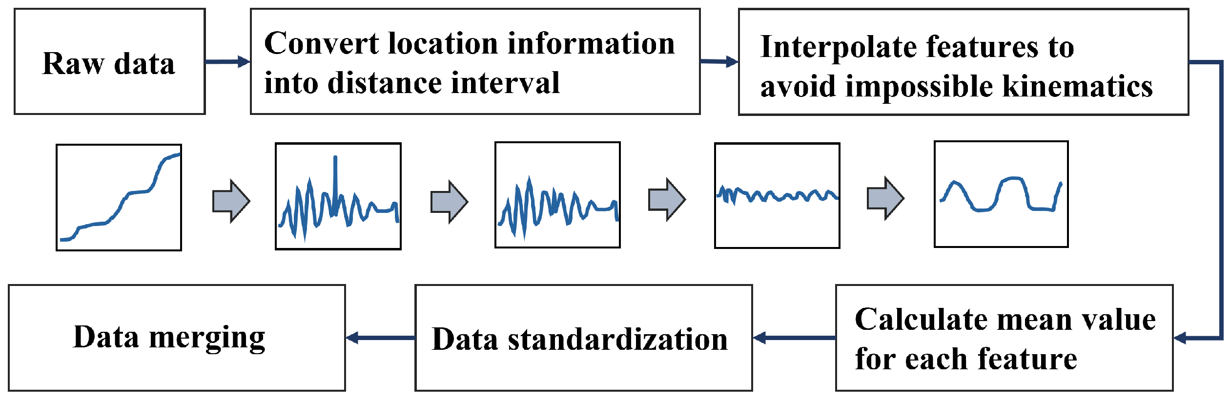
4.1. Data Processing

This study uses Chengdu Metro Line 6 data to generate our model. In order to accurately record the potential patterns of train operation, train data are collected at different times on the same track. The minimum and maximum velocities for the raw data sampling at 200 ms are 0 and 22.15 m/s, respectively. Therefore, we set the time of track prediction as when the train can cover the service breaking from the maximum speed in the next 15 s.
In our previous work, we made a preliminary data mutual promotion that the position data is processed within walking distance within the time interval. In order to test the generalization ability of the trajectory prediction model, these data sets are divided into two parts: the training set and the test set, and there is no data intersection. For example, 80% of the initial data of one dataset are used for training purposes, and the remaining 20% of the data are organized in the test set. Although we can get an accurate prediction when the future step size is less than 20 (the prediction time is less than 4 s), the prediction time of 15 s requires that the prediction step size be set to 75. In the simulation test in our debugging stage, we find that the prediction result in step 75 deviated significantly from the actual data, as shown in Figure 4a. Therefore, we preprocess the data to convert the original data set, as shown in Figure 5.
As shown in Figure 5, we detect the abnormal data (such as the speed suddenly dropping to 0) and interpolate the abnormal data points based on the nearby data. Then, these data are processed by data standardization because the difference in single-column data is a large gap. We normalized the data to reduce the impact of numerically large data on model learning. Finally, we convert five 200 ms data into one 1 s data, which means that our prediction of the future can be shortened from 75-time steps to 15-time steps. The prediction error for these processed data is shown in Figure 4b. The MAE value is calculated, detailed data as shown in Table 1; the proposed data process method achieved a more accurate and more minor error.

4.2. Comparative Analysis of Experimental Results

In our model parameter setting, we input 50 steps of historical data information to predict the position of N time steps in the future, where N changes from 1 to 15. We use three evaluation indicators to evaluate the accuracy of the four model prediction trajectories, as shown in Table 2. All the models in our experiment were set to the same network structure except the LSTM model. Each model includes an input layer, standardization layer, full connection layer, and output layer. RNN, GRU, and LSTM models are all set as three hidden layers, each layer contains 128 cells. In order to improve the generalization ability of the prediction model, a drop layer is added between the hidden layers.
Given 50 historical points, we report the Root Mean Square Error (RMSE), MAE, and Mean Absolute Percentage Error (MAPE) for the future 15 steps (15 s). The results in Table 2 demonstrate the superior performance of the LSTM-KF model in capturing long-range dependencies. In our previous work, we compared our proposed model with several standard deep learning models, such as RNN, GRU, and LSTM. When the prediction time step is increased to 15 steps, the MAPE of the lstm-kf model is 9.1%, while that of RNN and LSTM are 13.8% and 11.1%, respectively. It can be observed that the lstm-kf model has improved in MAE, RMSE, and MAPE compared with the LSTM model. Our model has apparent advantages in dealing with the long-time problem of train trajectory prediction.
According to the approach proposed in Section 3, We use real data to simulate the motion process of the pilot train and establish a dynamic model to control the operation of the rear vehicle. The simulation runs under the dynamic headway model and the traditional moving-block model, respectively, and the results are shown in Table 3.
In order to show the change of train headway in Table 3 clearly, the headways between two train trips in the optimized dynamic headway model and traditional moving block are calculated in Figure 6, where each time unit represents the operation time (s) in the experiment, and the track distance represents the distance (m) from the leading train minus the length of the body of the leading train. Comparing the dynamic headway mode and the traditional moving-block mode in the two cases, we find evidence to demonstrate the advantages and improvements of our proposed model. The train track distance of the proposed model could reach 27.5 m, while the minimum track distance of the traditional moving block is 100 m.
In case 1, the mean headway, max headway, and mean velocity of the proposed dynamic headway model are slightly higher than the traditional moving-block mode, while the actual distances between two trains of the dynamic headway model are much lower than the traditional moving-block mode.
A more detailed observation can be obtained from Figure 7; the following train runs faster under the dynamic headway policy than in the traditional moving-block mode.
Figure 6a shows that the real-time interval between the train and the leading train under the dynamic headway model is smaller than the traditional moving block, which proves that our method reduces the train-tracking distance and achieves higher density security tracking. In this case, case 2, the headway of our proposed model is 67% higher than the traditional moving-block model, and the actual distance of the dynamic headway model is 64.33% less than the traditional method. As shown in Figure 6, the actual distance between the trains under the dynamic headway model is presented with a trend of monotonous decline and rise as the increasing and decreasing of the interval between the gap between these two methods. The effect of the model in the case 1 experiment is not as prominent as case 2. The main possible reason is that the leading train in case 2 has a higher velocity, and the trajectory prediction can better compensate for the position and movement within the prediction time. In other words, our model is more efficient under higher-speed operating conditions.
The results indicate that the dynamic headway model based on the LSTM-KF trajectory prediction can improve the headway and reduce the track distance. The model achieved consistent and better results than the traditional moving-block mode. The results show that integrating long-time accurate trajectory prediction into headway calculation can generate a more advanced dynamic headway model.

5. Conclusions

In this study, a dynamic headway model based on the LSTM-KF trajectory prediction model is proposed for moving-block mode in the CBTC system. The future trajectory prediction of the train can be improved by the hybrid model that combined the LSTM of a deep learing model and the KF of a model-based method. Moreover, a dynamic headway policy for CBTC is proposed. We showed how to incorporate dynamic headway into the moving-block mode of trains to shorten train spacing and minimize running time.
Since the dynamic headway relies on communications, we also address the situation of temporary or permanent communication or permanent communication loss. We use the simulation model of Chengdu Metro Line 6 to demonstrate our proposed method. The results show that the running distance between trains is significantly shortened due to the use of our dynamic headway model. The track distance between two trains achieved a reduction of 69% on average. The dynamic headway model is believed to be also effective when considering emergencies due to the combination of deep learning and model-based methods for trajectory prediction and the security-oriented headway algorithm. Future works will concentrate on the security verification of the proposed model and some simulation-based test and algorithm optimization methods.

Author Contributions

Conceptualization, T.T.; methodology, Y.H.; software, J.L.; validation, Y.H. and J.L.; formal analysis, Y.H. and J.L.; investigation, Y.H. and J.L.; resources, Y.H. and J.L.; data curation, J.L.; writing—original draft preparation, Y.H.; writing—review and editing, Y.H. and J.L.; visualization, J.L.; supervision, Y.H. and J.L.; project administration, Y.H. and J.L.; funding acquisition, Y.H. All authors have read and agreed to the published version of the manuscript.

Funding

This research was funded by Beijing National Science Foundation (L201004, L211019).

Institutional Review Board Statement

Not applicable.

Informed Consent Statement

Not applicable.

Data Availability Statement

Not applicable.

Conflicts of Interest

The authors declare no conflict of interest.

References

  1. Quaglietta, E.; Wang, M.; Goverde, R. A multi-state train-following model for the analysis of virtual coupling railway operations. J. Rail Transp. Plan. Manag. 2020, 15, 100195. [Google Scholar] [CrossRef]
  2. Zhao, Y.; Ioannou, P. Positive Train Control with Dynamic Headway Based on an Active Communication System. IEEE Trans. Intell. Transp. Syst. 2015, 16, 3095–3103. [Google Scholar] [CrossRef]
  3. Niu, H.; Zhou, X.; Gao, R. Train scheduling for minimizing passenger waiting time with time-dependent demand and skip-stop patterns: Nonlinear integer programming models with linear constraints. Transp. Res. Part B 2015, 76, 117–135. [Google Scholar] [CrossRef]
  4. Khoshniyat, F.; Peterson, A. Improving train service reliability by applying an effective timetable robustness strategy. J. Intell. Transp. Syst. 2017, 21, 525–543. [Google Scholar] [CrossRef]
  5. Xun, J.; Li, K.P.; Cao, Y. An Optimization Approach for Real-Time Headway Control of Railway Traffic. IEICE Trans. Inf. Syst. 2015, E98D, 140–147. [Google Scholar] [CrossRef]
  6. Yang, X.; Li, X.; Ning, B.; Tang, T. An optimisation method for train scheduling with minimum energy consumption and travel time in metro rail systems. Transp. B 2015, 3, 79–98. [Google Scholar] [CrossRef]
  7. Li, S.; Schutter, B.D.; Yang, L.; Gao, Z. Robust Model Predictive Control for Train Regulation in Underground Railway Transportation. IEEE Trans. Control Syst. Technol. 2016, 24, 1075–1083. [Google Scholar] [CrossRef]
  8. Sanchez-Martinez, G.E.; Koutsopoulos, H.N.; Wilson, N. Real-time holding control for high-frequency transit with dynamics. Transp. Res. Part B Methodol. 2016, 83, 1–19. [Google Scholar] [CrossRef]
  9. Dong, H.; Gao, S.; Ning, B. Cooperative Control Synthesis and Stability Analysis of Multiple Trains Under Moving Signaling Systems. IEEE Trans. Intell. Transp. Syst. 2016, 17, 2730–2738. [Google Scholar] [CrossRef]
  10. Li, S.; Yang, L.; Gao, Z. Adaptive coordinated control of multiple high-speed trains with input saturation. Nonlinear Dyn. 2016, 3, 2157–2169. [Google Scholar] [CrossRef]
  11. Li, S.; Yang, L.; Gao, Z. Coordinated cruise control for high-speed train movements based on a multi-agent model. Transp. Res. Part C 2015, 56, 281–292. [Google Scholar] [CrossRef]
  12. Zhao, Y.; Wang, T.; Karimi, H.R. Distributed cruise control of high-speed trains. J. Frankl. Inst. 2017, 354, 6044–6061. [Google Scholar] [CrossRef]
  13. Ye, H.; Liu, R. A multiphase optimal control method for multi-train control and scheduling on railway lines. Transp. Res. Part B Methodol. 2016, 93, 377–393. [Google Scholar] [CrossRef]
  14. Ye, H.; Liu, R. Nonlinear programming methods based on closed-form expressions for optimal train control. Transp. Res. Part C Emerg. Technol. 2017, 82, 102–123. [Google Scholar] [CrossRef]
  15. Shi, F.; Zhao, S.; Zhou, Z.; Wang, P.; Bell, M. Optimizing train operational plan in an urban rail corridor based on the maximum headway function. Transp. Res. Part C Emerg. Technol. 2017, 74, 51–80. [Google Scholar] [CrossRef]
  16. Le, Z.; Li, K.; Ye, J.; Xu, X. Optimizing the train timetable for a subway system. Proc. Inst. Mech. Eng. Part F J. Rail Rapid Transit. 2015, 229, 852–862. [Google Scholar] [CrossRef]
  17. Zhou, Y.; Bai, Y.; Li, J.; Mao, B.; Li, T. Integrated Optimization on Train Control and Timetable to Minimize Net Energy Consumption of Metro Lines. J. Adv. Transp. 2018, 2018, 7905820. [Google Scholar] [CrossRef]
  18. Sangphong, O.; Siridhara, S.; Ratanavaraha, V. Determining Critical Rail Line Blocks and Minimum Train Headways for Equal and Unequal Block Lengths and Various Train Speed Scenarios. Eng. J. 2017, 21, 281–293. [Google Scholar] [CrossRef]
  19. Zhang, J.; Han, B. Research on the optimization of train headway for the high-speed railway network. In Proceedings of the ICSSSM11, Tianjin, China, 25–27 June 2011; pp. 1–6. [Google Scholar] [CrossRef]
  20. Li, X.; Zhang, B.; Liu, Y. A little bit flexibility on headway distribution is enough: Data-driven optimization of subway regenerative energy. Inf. Sci. 2021, 554, 276–296. [Google Scholar] [CrossRef]
  21. Kong, J.; Yang, C.; Wang, J.; Wang, X.; Zuo, M.; Jin, X.; Lin, S. Deep-Stacking Network Approach by Multisource Data Mining for Hazardous Risk Identification in IoT-Based Intelligent Food Management Systems. Comput. Intell. Neurosci. 2021, 2021, 1194565. [Google Scholar] [CrossRef]
  22. Liu, Q.; Wu, S.; Wang, L.; Tan, T. Predicting the Next Location: A Recurrent Model with Spatial and Temporal Contexts; AAAI Press: Palo Alto, CA, USA, 2016. [Google Scholar]
  23. Al-Molegi, A.; Jabreel, M.; Ghaleb, B. STF-RNN: Space-Time Features-based Recurrent Neural Network for Predicting People’s Next Location. In Proceedings of the Computational Intelligence, Athens, Greece, 6–9 December 2016. [Google Scholar]
  24. Kim, B.D.; Kang, C.M.; Lee, S.H.; Chae, H.; Kim, J.; Chung, C.C.; Choi, J.W. Probabilistic Vehicle Trajectory Prediction over Occupancy Grid Map via Recurrent Neural Network; IEEE: Piscataway, NJ, USA, 2017. [Google Scholar]
  25. Park, S.H.; Kim, B.D.; Kang, C.M.; Chung, C.C.; Choi, J.W. Sequence-to-Sequence Prediction of Vehicle Trajectory via LSTM Encoder-Decoder Architecture; IEEE: Piscataway, NJ, USA, 2018. [Google Scholar]
  26. Berenguer, A.D.; Alioscha-Perez, M.; Oveneke, M.C.; Sahli, H. Context-aware human trajectories prediction via latent variational model. IEEE Trans. Circuits. Syst. Video Technol. 2020, 31, 1876–1889. [Google Scholar] [CrossRef]
  27. Gao, C. Long Short-Term Memory Neural Network Applied to Train Dynamic Model and Speed Prediction. Algorithms 2019, 12, 173. [Google Scholar]
  28. Gupta, A.; Johnson, J.; Li, F.F.; Savarese, S.; Alahi, A. Social GAN: Socially Acceptable Trajectories with Generative Adversarial Networks. In Proceedings of the 2018 IEEE/CVF Conference on Computer Vision and Pattern Recognition (CVPR), Salt Lake City, UT, USA, 18–23 June 2018. [Google Scholar]
  29. Jin, X.B.; Gong, W.T.; Kong, J.L.; Bai, Y.T.; Su, T.L. PFVAE: A Planar Flow-Based Variational Auto-Encoder Prediction Model for Time Series Data. Mathematics 2022, 10, 610. [Google Scholar] [CrossRef]
  30. Chen, D.; Yan, X.; Liu, X.; Li, S.; Tian, X. A Multiscale-Grid-Based Stacked Bidirectional GRU Neural Network Model for Predicting Traffic Speeds of Urban Expressways. IEEE Access 2020, 9, 1321–1337. [Google Scholar] [CrossRef]
  31. Zhao, T.; Xu, Y.; Monfort, M.; Choi, W.; Baker, C.; Zhao, Y.; Wang, Y.; Wu, Y.N. Multi-Agent Tensor Fusion for Contextual Trajectory Prediction. In Proceedings of the IEEE/CVF Conference on Computer Vision and Pattern Recognition, Long Beach, CA, USA, 15–20 June 2019; IEEE: Piscataway, NJ, USA, 2019. [Google Scholar]
  32. Deo, N.; Trivedi, M.M. Convolutional Social Pooling for Vehicle Trajectory Prediction. In Proceedings of the 2018 IEEE/CVF Conference on Computer Vision and Pattern Recognition Workshops (CVPRW), Salt Lake City, UT, USA, 18–23 June 2018. [Google Scholar]
  33. He, Y.; Lv, J.; Zhang, D.; Chai, M.; Liu, H.; Dong, H.; Tang, T. Trajectory Prediction of Urban Rail Transit Based on Long Short-Term Memory Network. In Proceedings of the 2021 IEEE International Intelligent Transportation Systems Conference (ITSC), Indianapolis, IN, USA, 19–22 September 2021; pp. 3945–3950. [Google Scholar] [CrossRef]
Figure 1. Concrete and soft wall of CBTC system.
Actuators 11 00237 g001
Figure 2. Headway control loop.
Actuators 11 00237 g002
Figure 3. The process of trajectory prediction.
Actuators 11 00237 g003
Figure 4. The prediction error for 15 s. (a) The prediction error of 75 steps for 15 s. (b) The prediction error of 15 steps for 15 s.
Actuators 11 00237 g004
Figure 5. Data pre-processing procedure.
Actuators 11 00237 g005
Figure 6. The comparison of dynamic headway model and the traditional moving block. (a) The track distance between trains. (b) The track distance between trains.
Actuators 11 00237 g006
Figure 7. Illustration of comparison between the dynamic headway and the traditional moving block.
Actuators 11 00237 g007
Table 1. Prediction error for the processed data.
ErrorMaxmum (cm)Minimum (cm)Mean Error (cm)
75 steps—15 s1718−682.1251.00
15 steps—15 s165.31−150.839.38
Table 2. Trajectory prediction.
IndicatorsRMSEMAEMAPE
ModelRNNGRULSTMLSTM-KFRNNGRULSTMLSTM-KFRNNGRULSTMLSTM-KF
126.522.234.524.316.016.828.019.91.92.03.42.4
227.516.223.725.321.813.718.019.92.71.72.22.4
327.119.427.027.223.617.421.021.22.92.12.62.6
441.023.629.829.835.621.225.224.24.32.63.13.0
550.429.737.035.144.127.232.029.45.43.33.93.6
655.033.634.537.443.330.629.231.75.33.73.63.9
762.840.036.740.054.434.530.834.06.64.23.84.2
872.851.944.644.959.047.337.738.27.25.84.64.7
983.159.749.850.165.054.641.342.07.96.75.05.1
1093.266.557.356.376.259.447.847.09.37.25.85.7
11101.673.567.363.782.664.857.553.610.17.97.06.5
12112.083.967.069.292.173.355.057.911.28.96.77.1
13119.489.076.675.895.777.164.163.311.79.47.87.7
14122.199.580.481.8100.386.866.468.112.210.68.18.3
15137.6106.095.289.7112.990.780.874.713.811.19.99.1
Table 3. Performance comparsion.
CaseCase 1Case 2
Performance IndicatorTraditional Moving BlockDynamic HeadwayTraditional Moving BlockDynamic Headway
Track distance (m)184.6474.66319.22113.85
Min Track distance (m)99.6927.52106.1759.75
Mean Headway (m)146.15149.99220.34221.18
Max Headway (m)300.00306.53415.49696.43
Min Headway (m)99.6898.48102.2078.60
Mean Velocity (m/s)6.166.6611.8410.51
Max Velocity (m/s)12.9913.1917.7921.93
Min Velocity (m/s)0.000.001.001.00
Publisher’s Note: MDPI stays neutral with regard to jurisdictional claims in published maps and institutional affiliations.

