Adaptive Neural Control of a 2DOF Helicopter with Input Saturation and Time-Varying Output Constraint

Abstract

An adaptive neural control for uncertain 2DOF helicopter systems with input saturation and time-varying output constraints is provided. A radial basis function neural network is used to estimate the uncertainty terms present in the system. The saturation error and the external disturbance are considered as a composite disturbance, and an adaptive auxiliary parameter is introduced to compensate it. An asymmetric barrier Lyapunov function is employed to address the constraint violation of the system output. The closed-loop stability of the system is then demonstrated by Lyapunov theory analysis. Simulation results demonstrate the effectiveness of the control strategy.

1. Introduction

Helicopters not only have the characteristics of small size, strong adaptability, and ease of use, but also have the functions of vertical lifting, hovering, and low-altitude flight in a small area. They have been widely used in military investigation, civil transportation, surveying and mapping, and disaster relief [1,2,3]. However, the helicopter system is a highly nonlinear multiple-input, multiple-output (MIMO) system, and the difficulties of system control stability are exacerbated by the presence of uncertainties in the system, high coupling between axes, and time-varying parameters [4,5]. To improve the control stability of the helicopter system, it is practical to design an excellent robust control strategy.

Many control methods for helicopter systems have been proposed in the last few decades. These include linear quadratic regulator-based control, PID control, slip control, and fuzzy control [6,7,8,9]. For example, in [6], for a three-degree of freedom (DOF) helicopter model, the authors used LQR control to deal with the error system caused by the control strategy and linearization approximation. In [7], a new proportional-integral derivative controller based on a new quadrotor model was proposed and comparative tests demonstrated that the introduced nonlinear PID algorithm has good tracking accuracy. In [8], the attitude stabilization problem of a tilting three-rotor aircraft was solved by proposing a nonsingular timed sliding mode surface and designing a continuous fast timed sliding mode control law. In [9], the nonlinear behavior of the fuzzy controller and the absence of complex computations were used to test the performance of interference suppression for a single-azimuth helicopter model. However, in previous studies, the uncertainty in the helicopter system was neglected, which may lead to the design of helicopter control strategies that are not well suited for practical situations. Thus, the uncertainty of helicopter systems is necessary to be considered when designing high performance controllers.

In the last few years, researchers have proposed many outstanding control strategies for nonlinear systems with uncertainty [10,11,12]. For instance, in [11], subjected to unmodeled uncertainty in nonlinear systems, the authors presented a novel output feedback control strategy. In [12], an adaptive integral robust control method was designed in order to provide high precision trajectory tracking control of the two-bar hydraulic mechanism. Although there has been a good development of control research for nonlinear systems with uncertainty, these control strategies require very accurate system models. However, in practice, the models of many nonlinear systems are not usually accurate. Therefore, in recent years, neural network (NN) control has been used to solve the control of nonlinear systems with uncertainty [13,14]. Radial basis function NNs (RBFNNs) are widely used in control design for uncertain nonlinear systems due to their general approximation capability on compact sets [15]. For example, in [16], the RBFNN was used to eliminate the effects of input nonlinearities and external disturbances on the vibration problems of belt systems. In [17], to improve the tracking performance of the output force of the spacecraft, the authors developed an innovative multilayer NN adaptive control algorithm. In [18], the uncertainty and chattering problems of a nonlinear 2DOF helicopter control system were solved by NN approximation, and the trajectory tracking of the system was achieved. In [19], an adaptive neural fault-tolerant control strategy was presented for helicopter nonlinear systems with output error constraints and actuator failures. Although numerous NN control applications in helicopters and other nonlinear systems have been studied, few output constraints have been reported for helicopter systems, which prompts us to investigate further.

In practice, the output of helicopter systems is affected by various constraints, and violation of constraints may reduce the stability of the system and even lead to serious safety accidents [20]. Therefore, in order to overcome the effects of various constraints on the system output, researchers have proposed many brilliant control methods [21,22]. For example, in [23], the hybrid problem of input backlash and system uncertainty of a 2DOF helicopter nonlinear system model was dealt with by approximating the nonlinear error and unknown function used the RBFNN. In [24], the RBFNN was used to estimate the uncertainty of a 2DOF helicopter and solve the problem with unknown backlash-like hysteresis and output constraints. However, the output constraints mentioned above were studied for constant constraints, while in real situations, most of the systems were subjected to time-varying constraints, so it is necessary to examine the time-varying output constraints. In [25], for a nonlinear uncertain continuous stirred reactor model, a time-varying barrier Lyapunov function (TVBLF) was used to handle the time-varying output constraints to ensure that all signals in the system are bounded. In [26], an asymmetric time-varying BLF was designed to remove the effect of the time-varying output constraint and keep the deflection of the ship within the prescribed constraints. In [27], an NN control strategy with a prescribed performance function was developed in order to meet the output performance requirements of a real plant. Although there have been many studies on time-varying output constraints for the above-mentioned nonlinear systems, to our knowledge, there are few reports on time-varying output constraints for 2DOF helicopter systems. Moreover, in practical situations, neglecting input saturation may affect the system stability. Therefore, it is worthwhile to explore the design of a control strategy to compensate for the saturation nonlinearity for helicopter systems with input saturation.

In a real helicopter system, the input signal is always limited to a certain range due to the physical limitations of the actuator. Among them, input saturation is a common input constraint limitation in control design, and if the effect of saturation nonlinearity is neglected, it will lead to reduced control performance and stability of the system [28,29,30]. Therefore, researchers have conducted extensive investigations on the effects of input saturation. For instance, in [31], the authors introduced an auxiliary system to solve the input saturation problem in a quadrotor UAV trajectory tracking control scheme. In [32], the authors presented a discrete-time neural control of a quadrotor UAS with external disturbances and input saturation. In [33], the authors introduced an adaptive NN fault-tolerant control to solve the input saturation and external disturbances in an unmanned helicopter system. In [34], for quadrotor UAV tracking control with external disturbances and input saturation, an anti-jamming filter control was proposed. Although there have been abundant studies on the control of helicopters and other nonlinear systems with input saturation, few studies have been conducted for 2DOF helicopter systems with both time-varying output constraints and input saturation, which deserves further exploration.

With the above analysis and discussion, the objective of this paper is to propose an adaptive NN control for the 2DOF helicopter systems with time-varying output constraints and input saturation. The main contributions of this work compared to existing studies are as follows:

(i)

The time-varying output of the system is solved using TVBLF to keep the system output within a time-varying region.

(ii)

Unlike [28,29,30,32,33], in this study, we consider the input saturation error and external perturbation as a composite perturbation and compensate it using adaptive parameters.

(iii)

In the simulation results, the superiority of the control strategy proposed in this study is demonstrated based on the comparison results of multiple sets of simulations.

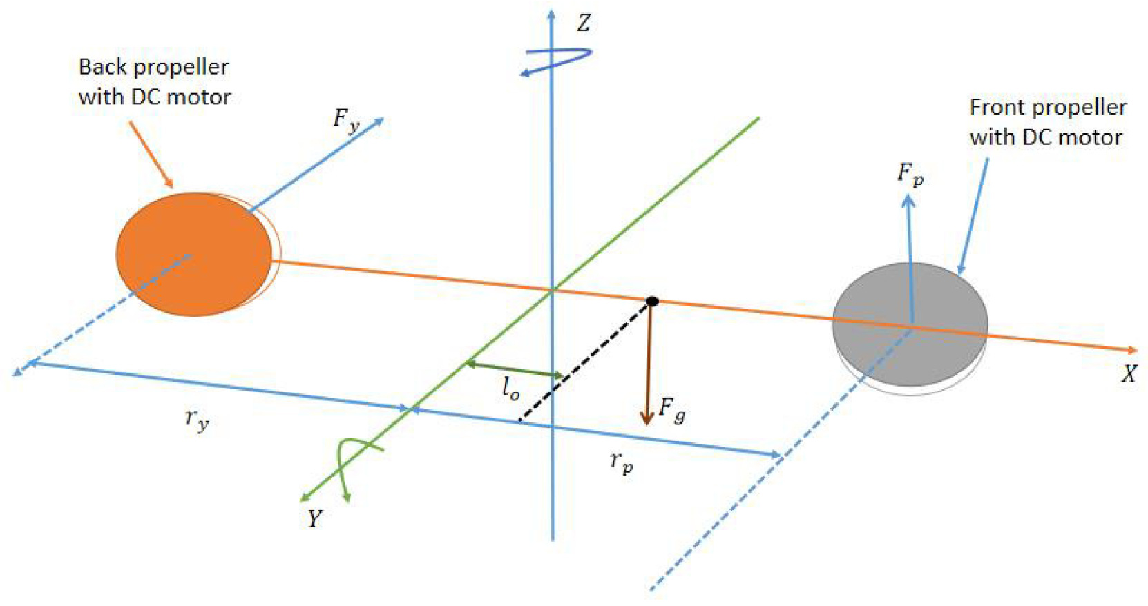
2. Problem Formulation and Preliminaries

2.1. Problem Formulation

Figure 1 displays the model for the 2DOF helicopter. Based on [35], we know the following equations for the dynamics of a 2DOF helicopter:

$$\begin{array}{cc}\hfill \ddot{\theta }& =\frac{-M_o{g}_o{l}_{o}cos\theta -D_{opp}\dot{\theta }-M_o{l}_o^2{\dot{\psi }}^{2}sin\theta cos\theta }{(J_{opp}+M_o{l}_o^2)}+\frac{K_{opp}{V}_p+K_{opy}{V}_y}{(J_{opp}+M_o{l}_o^2)},\hfill \end{array}$$

(1)

$$\begin{array}{cc}\hfill \ddot{\psi }& =\frac{-D_{oyy}\dot{\psi }+2M_o{l}_o^2\dot{\psi }\dot{\theta }sin\theta cos\theta }{(J_{oyy}+M_o{l}_o^2{cos}^2\theta )}+\frac{K_{oyp}{V}_p+K_{oyy}{V}_y}{(J_{oyy}+M_o{l}_o^2{cos}^2\theta )},\hfill \end{array}$$

(2)

where $\theta$ and $\psi$ denote pitch and yaw angle, respectively. $V_p$ and $V_y$ represent the voltages of the front and back motors, respectively. In addition, the parameters $M_o$, $g_o$, $l_o$, $D_{opp}$, $D_{oyy}$, $J_{opp}$, $J_{oyy}$, $K_{opp}$, $K_{opy}$, $K_{oyy}$, and $K_{oyp}$ are available in the Quanser Technical Manual [36].

Let $x={[x_1,x_2]}^T$, $x_1={[\theta ,\psi ]}^T$, and $x_2={[\dot{\theta },\dot{\psi }]}^T$. According to the 2DOF helicopter system, it can be converted to the general form of MIMO as follows:

$${\dot{x}}_1=x_2,$$

(3)

$${\dot{x}}_2=N\left(x\right)+\Delta N\left(x\right)+M\left(x\right)u+d\left(t\right),$$

(4)

$$y=x_1,$$

(5)

where $\Delta N\left(x\right)$ represents an unknown smooth function vector, $u={[V_p,V_y]}^T$ denotes the control input, and $d\left(t\right)$ is unknown external disturbance. Moreover, $N\left(x\right)$ and $M\left(x\right)$ are given by

$$\begin{array}{cc}\hfill N\left(x\right)& =\left[\begin{array}{c}\frac{-M_o{g}_o{l}_{o}cos\left(x_{11}\right)-D_{opp}{x}_{21}-M_o{l}_o^2{\dot{x}}_{22}^{2}sin\left(x_{11}\right)cos\left(x_{11}\right)}{J_{opp}+M_o{l}_o^2}\\ \frac{-D_{oyy}{x}_{22}+2M_o{l}_o^2{x}_{22}{x}_{21}sin\left(x_{11}\right)cos\left(x_{11}\right)}{J_{oyy}+M_o{l}_o^2{cos}^2\left(x_{11}\right)}\end{array}\right],\hfill \end{array}$$

(6)

$$\begin{array}{cc}\hfill M\left(x\right)& =\left[\begin{array}{cc}\frac{K_{opp}}{J_{opp}+M_o{l}_o^2}& \frac{K_{opy}}{J_{opp}+M_o{l}_o^2}\\ \frac{K_{oyp}}{J_{oyy}+M_o{l}_o^2{cos}^2\left(x_{11}\right)}& \frac{K_{oyy}}{J_{oyy}+M_o{l}_o^2{cos}^2\left(x_{11}\right)}\end{array}\right].\hfill \end{array}$$

(7)

Remark 1. 

The aim is to design a controller in such a way that the output of the system follows the desired trajectory, $x_d$, while ensuring that the time-varying output constraint is not violated. In this paper, the system output is constrained as

$$\begin{array}{c}\hfill {\underline{\kappa }}_c\left(t\right)\le x_1\le {\overline{\kappa }}_c\left(t\right),\forall t\ge 0,\end{array}$$

(8)

where ${\underline{\kappa }}_c={[{\underline{\kappa }}_{c1},{\underline{\kappa }}_{c2}]}^T$ and ${\overline{\kappa }}_c={[{\overline{\kappa }}_{c1},{\overline{\kappa }}_{c2}]}^T$.

Consider the channel control input $u={[u_1,u_2]}^T$ subject to the following constraints:

$$\begin{array}{c}\hfill u_{Li}\le u_i\le u_{Hi},i=1,2,\end{array}$$

(9)

where $u_{Li}$ and $u_{Hi}$ are the upper and lower bounds of the control inputs. Thus, the control input $u_i$ is defined as

$$\begin{array}{c}\hfill u_i=\left\{\begin{array}{cc}{u}_{Hi}\hfill & \mathrm{if}{u}_i\ge u_{Hi}\hfill \\ u_{0i}\hfill & \mathrm{if}{u}_{Li}\le u_{0i}<u_{Hi}\hfill \\ u_{Li}\hfill & \mathrm{if}{u}_{0i}<u_{Li}.\hfill \end{array}\right.\end{array}$$

(10)

The control input u is rewritten as

$$\begin{array}{c}\hfill u=u_0+u_{\Delta },\end{array}$$

(11)

where $u_0={[u_{01},u_{02}]}^T$ is the controller input signal to be designed later, and the unknown part $u_{\Delta }$ is expressed as

$$\begin{array}{c}\hfill u_{\Delta }=\left\{\begin{array}{cc}{u}_{Hi}-u_{0i}\hfill & \mathrm{if}{u}_i\ge u_{Hi}\hfill \\ u_{0i}\hfill & \mathrm{if}{u}_{Li}\le u_{0i}<u_{Hi}\hfill \\ u_{Li}-u_{0i}\hfill & \mathrm{if}{u}_{0i}<u_{Li}.\hfill \end{array}\right.\end{array}$$

(12)

Substituting (11) into (4), we derive

$$\begin{array}{cc}\hfill {\dot{x}}_2& =N\left(x\right)+\Delta N\left(x\right)+M\left(x\right)u_0+M\left(x\right)u_{\Delta }+d\left(t\right).\hfill \end{array}$$

(13)

2.2. Preliminaries

Assumption A1 

([37]). The gain function $M\left(x\right)$ satisfies $\parallel M\left(x\right)\parallel \le \overline{M}$ with $\overline{M}$ being a positive constant.

Assumption A2 

([38]). Based on a practical environment, it is assumed that the external disturbance $d\left(t\right)$ is continuous and bounded.

Assumption A3 

([39]). We suppose that the unknown part $u_{\Delta }$ is bounded and satisfies $\left|\right|u_{\Delta }\left|\right|\le {\overline{u}}_{\Delta }$ with ${\overline{u}}_{\Delta }>0$ being an unknown constant.

Lemma 1 

([40]). For any $q\in R$ that satisfies $\left|x\right|<\left|q\right|$ and $x\in R$, the following inequalities hold:

$$\begin{array}{c}\hfill ln\frac{q^2}{q^2-x^2}\le \frac{x^2}{q^2-x^2}.\end{array}$$

(14)

Lemma 2 

([41]). For a continuous smooth function, we can use RBFNN to estimate the following:

$$\begin{array}{c}\hfill p\left(Z\right)={\Psi }^T\Phi \left(Z\right),\end{array}$$

(15)

where $\Phi \left(Z\right)={[{\Phi }_1\left(Z\right),{\Phi }_2\left(Z\right),\dots ,{\varphi }_m\left(Z\right)]}^T$ represents the basis function. In addition, $\Psi \in R^m$ and $Z\in R^q$ are the weight and input vector of the RBFNN, respectively.

As is well known, the RBFNN has the advantage of fast learning and strong estimation capability, so that the unknown continuous smooth function $p\left(Z\right)$ can be represented as

$$\begin{array}{c}\hfill p\left(Z\right)={\Psi }^{*T}\Phi \left(Z\right)+\delta \left(Z\right),\left|\right|\delta \left(Z\right)\left|\right|\le \overline{\delta },\end{array}$$

(16)

where ${\Psi }^{*}$ denotes an ideal weight vector, $\delta \left(Z\right)$ is an approximation error, and $\overline{\delta }$ is an unknown positive constant.

Lemma 3 

([42]). For $\varpi >0$ and $a\in R$, the following inequality holds

$$\begin{array}{c}\hfill 0\le \left|a\right|-atanh(\frac{a}{\varpi })\le 0.2785\varpi .\end{array}$$

(17)

3. Controller Design and Stability Analysis

We define the first error variable as $z_1\left(t\right)=x_1\left(t\right)-x_d\left(t\right)$, where $x_d\left(t\right)={[x_{d1}\left(t\right),x_{d2}\left(t\right)]}^T$ is the desired trajectory. The time derivative of $z_1\left(t\right)$ is given as

$$\begin{array}{c}\hfill {\dot{z}}_1\left(t\right)={\dot{x}}_1\left(t\right)-{\dot{x}}_d\left(t\right).\end{array}$$

(18)

We define the second error variable as $z_2\left(t\right)=x_2\left(t\right)-\alpha \left(t\right)$, where $\alpha \left(t\right)={[{\alpha }_1\left(t\right),{\alpha }_2\left(t\right)]}^T$ is a virtual control signal. The time derivative of $z_2\left(t\right)$ is given by

$$\begin{array}{c}\hfill {\dot{z}}_2\left(t\right)={\dot{x}}_2\left(t\right)-\dot{\alpha }\left(t\right).\end{array}$$

(19)

The time-varying boundary of $z_1$ is

$$\begin{array}{c}\hfill {\kappa }_a\left(t\right)\le z_1\left(t\right)\le {\kappa }_b\left(t\right),\end{array}$$

(20)

where ${\kappa }_a\left(t\right)=x_d\left(t\right)-{\underline{\kappa }}_c\left(t\right)$ and ${\kappa }_b\left(t\right)={\overline{\kappa }}_c\left(t\right)-x_d\left(t\right)$. Consider a TVBLF as follows [43]:

$$\begin{array}{c}\hfill V_1=\sum _{i=1}^2(\frac{h\left(i\right)}{2}ln\frac{{\kappa }_{bi}^2}{{\kappa }_{bi}^2+z_{1i}^2}-\frac{1-h\left(i\right)}{2}ln\frac{{\kappa }_{ai}^2}{{\kappa }_{ai}^2-z_{1i}^2}),\end{array}$$

(21)

where

$$\begin{array}{c}\hfill h\left(i\right)=\left\{\begin{array}{cc}0\hfill & \mathrm{if}{z}_{1i}\le 0\hfill \\ 1\hfill & \mathrm{if}{z}_{1i}>0.\hfill \end{array}\right.\end{array}$$

(22)

Define the transformation of error coordinates as follows:

$$\begin{array}{c}\hfill {\xi }_{ai}=\frac{z_{1i}}{{\kappa }_{ai}},{\xi }_{bi}=\frac{z_{1i}}{{\kappa }_{bi}},{\xi }_i=h\left(i\right){\xi }_{bi}+(1-h\left(i\right)){\xi }_{bi}.\end{array}$$

(23)

We rewrite (21) as follows [43]:

$$\begin{array}{c}\hfill V_1=\sum _{i=1}^2(\frac{1}{2}ln\frac{1}{1-{\xi }_i^2}).\end{array}$$

(24)

We know from (22) and (23) that $|{\xi }_i|<1$. In addition, the time derivative of $V_1$ is given as

$$\begin{array}{cc}\hfill {\dot{V}}_1& =\sum _{i=1}^2(\frac{{\xi }_{bi}h\left(i\right)}{(1-{\xi }_{bi}^2){\kappa }_{bi}}(z_{2i}+{\alpha }_i-{\dot{x}}_{di}-z_{1i}\frac{{\dot{\kappa }}_{bi}}{{\kappa }_{bi}})\hfill \\ & +\frac{{\xi }_{ai}h\left(i\right)}{(1-{\xi }_{ai}^2){\kappa }_{ai}}(z_{2i}+{\alpha }_i-{\dot{x}}_{di}-z_{1i}\frac{{\dot{\kappa }}_{ai}}{{\kappa }_{ai}})).\hfill \end{array}$$

(25)

The virtual control signal is designed as

$$\begin{array}{cc}\hfill \alpha & =\left[\begin{array}{c}{x}_{d1}-k_{11}{z}_{11}-{\overline{k}}_{11}{z}_{11}\\ x_{d2}-k_{12}{z}_{12}-{\overline{k}}_{12}{z}_{12}\end{array}\right],\hfill \end{array}$$

(26)

and

$$\begin{array}{c}\hfill {\overline{k}}_{1i}=\sqrt{{\gamma }_i+{(\frac{{\dot{\kappa }}_{bi}}{{\kappa }_{bi}})}^2+{(\frac{{\dot{\kappa }}_{ai}}{{\kappa }_{ai}})}^2},\end{array}$$

(27)

where ${\gamma }_i$ is a small positive constant. In addition, inserting (26) and (27) into (25), we obtain

$$\begin{array}{cc}\hfill {\dot{V}}_1& =\sum _{i=1}^2(\frac{{\xi }_{bi}h\left(i\right)}{(1-{\xi }_{bi}^2){\kappa }_{bi}}(z_{2i}-c_{1i}{z}_{1i}-({\overline{k}}_{1i}+\frac{{\dot{\kappa }}_{bi}}{{\kappa }_{bi}})z_{1i})\hfill \\ & +\frac{{\xi }_{ai}h\left(i\right)}{(1-{\xi }_{ai}^2){\kappa }_{ai}}(z_{2i}-c_{1i}{z}_{1i}-({\overline{k}}_{1i}+\frac{{\dot{\kappa }}_{ai}}{{\kappa }_{ai}})z_{1i}))\hfill \\ \hfill & \le -\sum _{i=1}^2{c}_{1i}\frac{{\xi }_i^2}{1-{\xi }_i^2}+\sum _{i=1}^2{\phi }_i{z}_{1i}{z}_{2i},\hfill \end{array}$$

(28)

where ${\phi }_i$ is set to

$$\begin{array}{c}\hfill {\phi }_i=(\frac{h\left(i\right)}{{\kappa }_{bi}^2-z_{1i}^2}+\frac{1-h\left(i\right)}{{\kappa }_{ai}^2-z_{1i}^2}),\end{array}$$

(29)

and $\phi =\mathrm{diag}\{{\phi }_1,{\phi }_2\}$.

Substituting (13) into (19) yields

$$\begin{array}{cc}\hfill {\dot{z}}_2& =N\left(x\right)+\Delta N\left(x\right)+M\left(x\right)u_0+M\left(x\right)u_{\Delta }+d\left(t\right)-\dot{\alpha }\left(t\right)\hfill \\ \hfill & =N\left(x\right)+M\left(x\right)u_0+M\left(x\right)u_{\Delta }+d\left(t\right)+P(x,t),\hfill \end{array}$$

(30)

where $P(x,t)=\Delta N\left(x\right)-\dot{\alpha }$. Since $\Delta N\left(x\right)$ is an unknown smooth function vector, we use NN to estimate it:

$$\begin{array}{c}\hfill P(x,t)={\Psi }^{*T}\Phi \left(Z\right)+\delta \left(Z\right),\end{array}$$

(31)

where $Z={[x_1^T,x_2^T,{\dot{x}}_d^T,{\ddot{x}}_d^T,{\alpha }^T]}^T$ and ${\Psi }^{*}$ are the input and weight vectors of the NN, respectively. In addition, $\delta \left(Z\right)$ is the approximation error and satisfies $\left|\right|\delta \left(Z\right)\left|\right|\le \overline{\delta }$ with $\overline{\delta }$ being an unknown positive constant. Substituting (31) into (30), we obtain

$$\begin{array}{cc}\hfill {\dot{z}}_2& =N\left(x\right)+M\left(x\right)u_0+M\left(x\right)u_{\Delta }+d\left(t\right)+{\Psi }^{*T}\Phi \left(Z\right)+\delta \left(Z\right)\hfill \\ \hfill & =N\left(x\right)+M\left(x\right)u_0+{\Psi }^{*T}\Phi \left(Z\right)+D(x,t)+\delta \left(Z\right),\hfill \end{array}$$

(32)

where $D(x,t)=M\left(x\right)u_{\Delta }+d\left(t\right)$.

Remark 2. 

According to Assumption 1, we know that $M\left(x\right)$ is bounded and satisfies $\left|\right|M\left(x\right)\left|\right|\le \overline{M}$, with $\overline{M}$ being an unknown positive constant. Based on Assumption 2, we know that $d\left(t\right)$ is bounded. From Assumption 3, we conclude that $u_{\Delta }$ is bounded and satisfies $\left|\right|u_{\Delta }\left|\right|\le {\overline{u}}_{\Delta }$, with ${\overline{u}}_{\Delta }>0$ being an unknown constant.

Define $\tilde{\Psi }=\widehat{\Psi }-{\Psi }^{*}$ and $\tilde{\overline{D}}=\overline{D}-\widehat{\overline{D}}$. We design the controller input as follows:

$$\begin{array}{c}\hfill u_0=-M^{-1}(N+{\widehat{\Psi }}^T\Phi \left(Z\right)+\widehat{\overline{D}}tanh(\frac{z_2}{d_0})+\phi z_1+c_2{z}_2).\end{array}$$

(33)

Then, the adaptive laws are designed as

$$\begin{array}{c}\hfill \dot{\widehat{\Psi }}={\Gamma }_1(\Phi \left(Z\right)z_2^T-{\eta }_1\widehat{\Psi }),\end{array}$$

(34)

$$\begin{array}{c}\hfill \dot{\widehat{\overline{D}}}={\Gamma }_2(z_2^{T}tanh(\frac{z_2}{d_0})-{\eta }_2\widehat{\overline{D}}),\end{array}$$

(35)

where ${\Gamma }_1={\Gamma }_1^T\in R^{2\times 2}$ is a diagonal matrix, and ${\eta }_1>0$, ${\Gamma }_2>0$, ${\eta }_2>0$, and $d_0>0$ are design parameters.

Based on the adaptive neural control strategy designed above, we derive the following theorem.

Theorem 1. 

Considering a 2DOF helicopter system with input saturation and time-varying output constraints, we propose an adaptive neural control strategy. The update law of the adaptive parameters is (35), the update law of the NN weights is (34), and the controller input for adaptive neural control is (33). With the developed control strategy, the control signals in the closed-loop system are all consistently bounded. In addition, the outputs of the system remain with time constraints, and no constraints are violated.

Proof. 

Consider the Lyapunov function as follows:

$$\begin{array}{c}\hfill V_2=V_1+\frac{1}{2}{z}_2^T{z}_2+\frac{1}{2}\mathrm{tr}\{{\tilde{\Psi }}^T{\Gamma }_1^{-1}\tilde{\Psi }\}+\frac{1}{2{\Gamma }_2}{\tilde{\overline{D}}}^2.\end{array}$$

(36)

Substituting (32)–(35) into the time derivative of $V_2$ gives

$$\begin{array}{cc}\hfill {\dot{V}}_2& ={\dot{V}}_1+z_2^T{\dot{z}}_2+\mathrm{tr}\{{\tilde{\Psi }}^T{\Gamma }_1^{-1}\dot{\widehat{\Psi }}\}-\frac{1}{{\Gamma }_2}\tilde{\overline{D}}\dot{\widehat{\overline{D}}}\hfill \\ \hfill & \le {\dot{V}}_1-z_2^T{\tilde{\Psi }}^T\Phi \left(Z\right)-z_2^T\widehat{\overline{D}}tanh(\frac{z_2}{d_0})-z_2^T\phi z_1-z_2^T{c}_2{z}_2\hfill \\ & +z_2^{T}D+z_2^T\delta \left(Z\right)+\mathrm{tr}\{{\tilde{\Psi }}^T(\Phi \left(Z\right)z_2^T-{\eta }_1\widehat{\Psi })\}\hfill \\ & -\tilde{\overline{D}}(z_2^{T}tanh(\frac{z_2}{d_0})-{\eta }_2\widehat{\overline{D}}).\hfill \end{array}$$

(37)

We regard an inequality as follows:

$$\begin{array}{c}\hfill z_2^{T}D\le \sum _{i=1}^2\left|z_{2i}\right|\overline{D}.\end{array}$$

(38)

In addition, one has

$$\begin{array}{c}\hfill z_2^{T}tanh(\frac{z_2}{d_0})=\sum _{i=1}^2(z_{2i}tanh(\frac{z_{2i}}{d_0})).\end{array}$$

(39)

According to Lemma 3, we obtain

$$\begin{array}{c}\hfill \sum _{i=1}^2\left|z_{2i}\right|-\sum _{i=1}^2(z_{2i}tanh(\frac{z_{2i}}{d_0}))\le 0.557d_0.\end{array}$$

(40)

Putting (38)–(40) into (37) yields

$$\begin{array}{cc}\hfill {\dot{V}}_2& \le {\dot{V}}_1-z_2^T\phi z_1-z_2^T{c}_2{z}_2+z_2^T\delta \left(Z\right)-{\eta }_1\mathrm{tr}\{{\tilde{\Psi }}^T\widehat{\Psi }\}\hfill \\ & +0.557d_0\overline{D}+{\eta }_2\tilde{\overline{D}}\overline{D}-{\eta }_2{\tilde{\overline{D}}}^2.\hfill \end{array}$$

(41)

Applying Youth’s inequalities, one can obtain

$$\begin{array}{cc}\hfill -{\eta }_1\mathrm{tr}\{{\tilde{\Psi }}^T\widehat{\Psi }\}& \le -\frac{{\eta }_1}{2}\left|\right|\tilde{\Psi }{\left|\right|}_F^2+\frac{{\eta }_1}{2}\left|\right|{\Psi }^{*}{\left|\right|}_F^2,\hfill \end{array}$$

(42)

$$\begin{array}{cc}\hfill \tilde{\overline{D}}\overline{D}& \le \frac{1}{\iota }{\tilde{\overline{D}}}^2+\iota {\overline{D}}^2,\hfill \end{array}$$

(43)

$$\begin{array}{cc}\hfill z_2^T\left(Z\right)\delta & \le \frac{1}{2}{z}_2^T{z}_2+\frac{1}{2}{\overline{\delta }}^2.\hfill \end{array}$$

(44)

Inserting (28) and (42)–(44) into (41) and invoking Lemma 1, we can obtain

$$\begin{array}{cc}\hfill {\dot{V}}_2& \le \sum _{i=1}^2{c}_{1i}ln\frac{1}{1-{\xi }_i^2}-z_2^T(c_2-\frac{1}{2}{I}_{2\times 2})z_2-\frac{{\eta }_1}{2}\left|\right|\tilde{\Psi }{\left|\right|}_F^2\hfill \\ & -{\eta }_2(1-\frac{1}{\iota }){\tilde{\overline{D}}}^2+0.557d_0\overline{D}+\frac{{\eta }_1}{2}\left|\right|{\Psi }^{*}{\left|\right|}_F^2+\iota {\overline{D}}^2+\frac{1}{2}{\overline{\delta }}^2\hfill \\ \hfill & \le -\beta V_2+H,\hfill \end{array}$$

(45)

where

$$\begin{array}{cc}\hfill \beta =& min\{2{\lambda }_{min}\left(c_{1i}\right),2{\lambda }_{min}(c_2-\frac{1}{2}{I}_{2\times 2}),\frac{{\eta }_1}{{\lambda }_{max}({\Gamma }_1^{-1})},\hfill \end{array}$$

$$\begin{array}{c}\hfill 2{\Gamma }_2{\eta }_2(1-\frac{1}{\iota })\},\end{array}$$

(46)

$$\begin{array}{cc}\hfill H& =0.557d_0\overline{D}+\frac{{\eta }_1}{2}\left|\right|{\Psi }^{*}{\left|\right|}_F^2+\iota {\overline{D}}^2+\frac{1}{2}{\overline{\delta }}^2.\hfill \end{array}$$

(47)

In order to ensure that the closed-loop system is bounded, the parameters $c_{1i}$, $c_2$, ${\eta }_1$, ${\Gamma }_2$, and ${\eta }_2$ need to satisfy the following conditions:

$$\begin{array}{c}\hfill {\lambda }_{min}\left(c_{1i}\right)>0,{\lambda }_{min}(c_2-\frac{1}{2}{I}_{2\times 2})>0,\\ \hfill {\eta }_1>0,2{\Gamma }_2{\eta }_2(1-\frac{1}{\iota })>0.\end{array}$$

(48)

According to (45), we know that $z_1$, $z_2$, $\tilde{\Psi }$, and $\tilde{\overline{D}}$ are bounded. Moreover, invoking (45), we obtain

$$\begin{array}{c}\hfill 0\le V_2\le \frac{H}{\beta }+[V_2\left(0\right)-\frac{H}{\beta }]e^{-\beta t}.\end{array}$$

(49)

Considering (45), we derive $\underset{t\to \infty }{lim}{V}_2=\frac{H}{\beta }$, which yields that $V_2$ is bounded. Thus, $z_1$, $z_2$, $\tilde{\Psi }$, and $\tilde{\overline{D}}$ are uniformly bounded. Furthermore, according to (8) and (49), we know that the output variable $x_1$ of the system eventually converges to a smaller domain and does not violate the time-varying constraints. □

4. Simulation

For the 2DOF helicopter system represented by (1)–(5), simulations are conducted to prove the effectiveness of the developed adaptive NN control strategy.

Table 1. System parameters.

Symbol	Parameter	Value	Unit
$J_{opp}$	Pitch axis moment of inertia	0.0215	kg · m2
$J_{oyy}$	Yaw axis moment of inertia	0.0237	kg · m2
$M_o$	Weight of the body	1.0750	kg
$D_{opp}$	Pitch axial coefficient of viscous friction	0.0071	N/V
$D_{oyy}$	Yaw axial coefficient of viscous friction	0.0220	N/V
$l_o$	Length from the center of mass to the fixing point of the body frame	0.002	m
$K_{opp}$	Torque thrust gain	0.022	N·m/V
$K_{opy}$	Torque thrust gain	0.0221	N·m/V
$K_{oyp}$	Torque thrust gain	−0.0227	N·m/V
$K_{oyy}$	Torque thrust gain	0.0022	N·m/V
$g_o$	Gravitational acceleration	9.8	m/s2

represents the parameters of the 2DOF helicopter system. Moreover, we choose the initial value of the output variable to be $x_1\left(0\right)={[0.5,0.8]}^T$ (rad/s), and the desired trajectory is selected as $x_d={[1.4sin\left(0.5t\right),1.4cos\left(0.5t\right)]}^T$ (rad/s).

The design parameters in this control strategy are selected as $c_{11}=10$, $c_{12}=15$, $c_2=\mathrm{diag}\{15,15\}$, ${\Gamma }_1=64I_{64\times 64}$, ${\sigma }_1=0.1$, ${\Gamma }_2=1$, ${\sigma }_2=0.05$, $d_0=0.5$, and ${\gamma }_i=0.1$, $i=1,2$. In the time-varying output constraint, we choose ${\underline{\kappa }}_c={[-1.1+0.4sin\left(0.5t\right),-1.1+0.4cos\left(0.5t\right)]}^T$ and ${\overline{\kappa }}_c={[2+0.6cos\left(0.5t\right),2+0.6sin\left(0.5t\right)]}^T$. The external disturbance is selected as $d\left(t\right)={[1.5+0.3sin\left(t\right),1.8+0.9cos\left(t\right)]}^T$. The parameters of input saturation are chosen as $u_{Hi}=24$ and $u_{Li}=-24$, $i=1,2$.

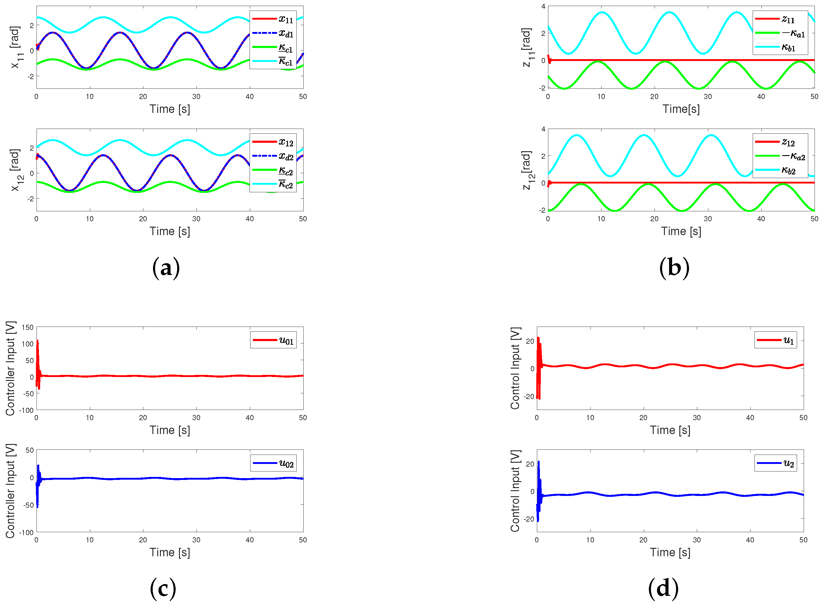
4.1. Case 1: Under the Proposed Control

Figure 2a represents the response of the output variable following the desired signal and that the output variables do not violate the time-varying constraint. Figure 2b shows the response of the tracking errors and satisfies ${\kappa }_a\le z_1\le {\kappa }_b$. Figure 2c,d depict the controller and control input signal, respectively. As can be seen from Figure 2d, the control input generates a large voltage at the start of system operation. However, the antisaturation compensator keeps the voltage within a certain range, while the system maintains good stability. In summary, the control strategy proposed in this study is both effective and reliable.

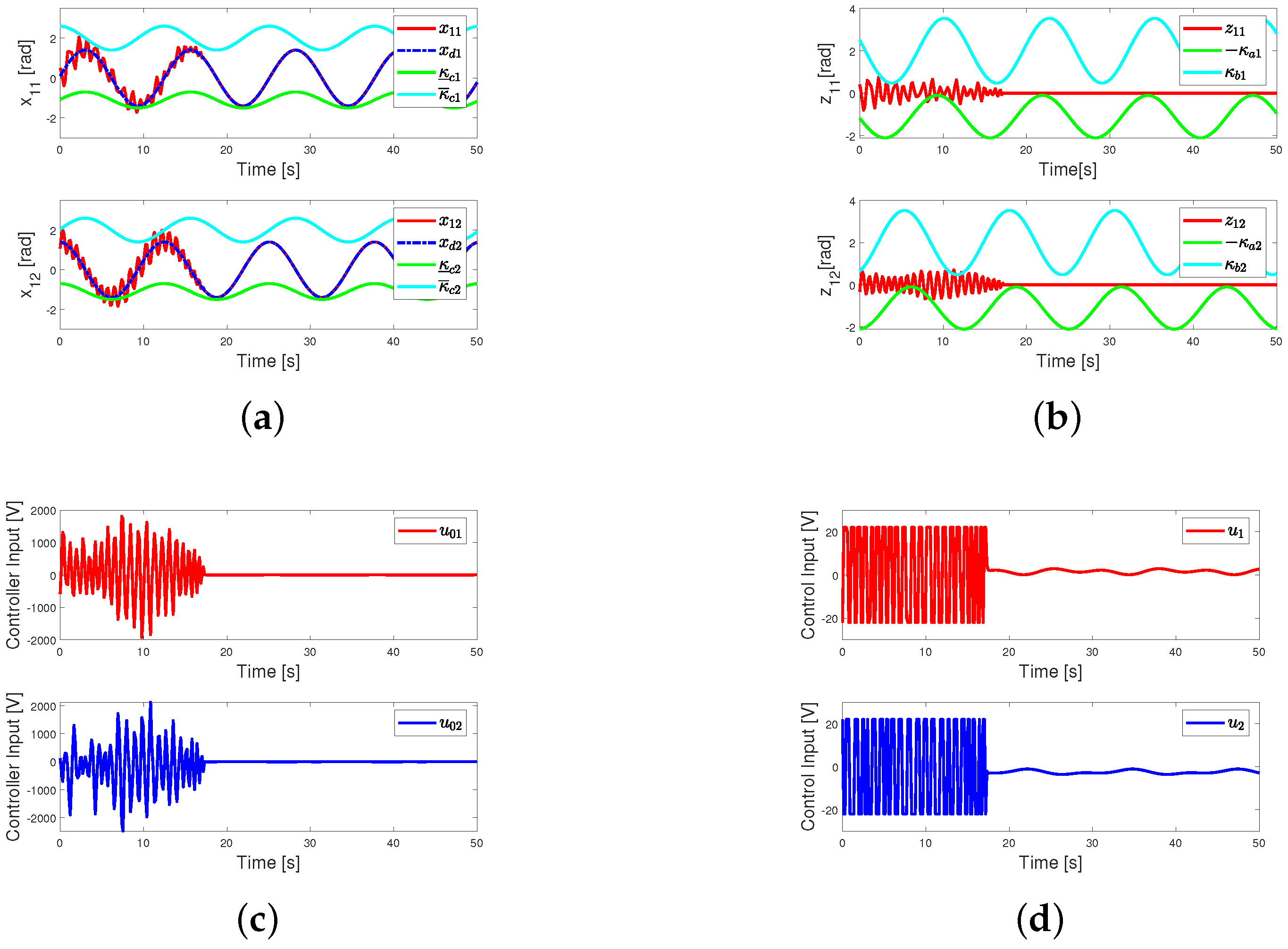
4.2. Case 2: Under the Proposed Control without Time-Varying Output Constraint

We disregard the time-varying output constraint in this case in order to demonstrate the superiority of Case 1. In addition, we choose the same design parameters as in Case 1. Figure 3a indicates the tracking response of the output variables against the desired trajectory. The tracking errors are shown in Figure 3b. The performance of the controller and control input signals are illustrated in Figure 3c,d.

In contrast to Case 1, we know that, when the condition of time-varying constraint is not regarded, the output variables of the system violate the constraint several times over a longer period of time at the beginning of the system run, and the tracking errors do not satisfy ${\kappa }_a\le z_1\le {\kappa }_b$. From Figure 3c, the controller input produces a larger overshoot over a long period of time. The control input in Figure 3d has an antisaturation effect for a period of 0–18 s, which may make the system very unstable during operation.

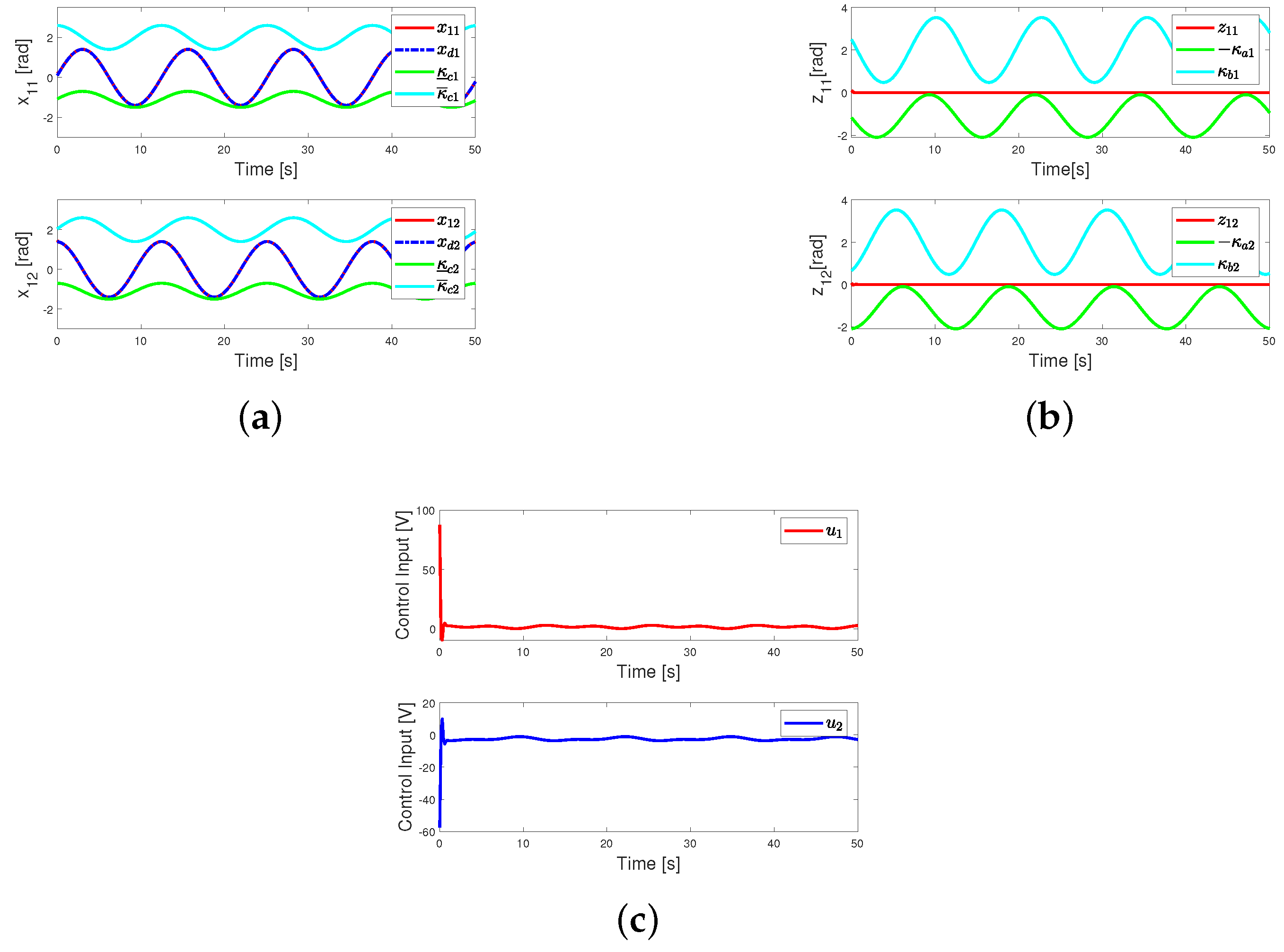
4.3. Case 3: Under the Proposed Control without Input Saturation

The impact of saturation nonlinearity is not considered in this subsection. According to (4), we can treat the external disturbance and the error of the NN as a composite disturbance D and compensate it using bounded estimation and a smooth function.

Let

$$\begin{array}{c}\hfill {\zeta }_{max}=\underset{t\ge 0}{sup}\left|\right|D\left|\right|\end{array}$$

(50)

We consider the following inequality

$$\begin{array}{c}\hfill z_2^{T}D\le j{z}_2^T{z}_2+\frac{1}{4j}{\zeta }_{max}^2.\end{array}$$

(51)

where j is a design parameter.

The adaptive neural controller is designed as follows:

$$\begin{array}{c}\hfill u=-M^{-1}(N+{\widehat{\Psi }}^T\Phi \left(Z\right)+\phi z_1+c_2{z}_2+j{z}_2)\end{array}$$

(52)

where the design parameters of the system are selected as $c_{11}=10$, $c_{12}=18$, $c_2=\mathrm{diag}\{20,20\}$, and $j=0.5$, and other design parameters remain the same as Case 1.

Figure 4a–c show the simulation results of Case 3. The tracking performance of the system output variables with respect to the desired signal is presented in Figure 4a. Figure 4b,c indicate the tracking errors and control input performance.

Although in the proposed control strategy the output variables do not violate the time-varying constraint boundaries, the control input to the system generates a large overshoot at the beginning, potentially leading to an excessive input voltage to the system with no antisaturation compensator for regulation, which could make the system operation unstable or even damage the components of the helicopter system.

5. Conclusions

An adaptive neural control scheme was proposed considering the effects of time-varying output constraints and input saturation. The RBFNN was used to estimate the uncertainty in the system. The saturation error and external disturbances were considered as composite disturbances and an adaptive auxiliary parameter was introduced to compensate it. The effect of time-varying output was handled using TVBLF. The Lyapunov stability proved that the closed-loop system was bounded. Finally, simulation results verified the superiority and effectiveness of the control strategy proposed in this study. Motivated by [44,45], in the future, we will focus on the study of model-free sliding mode control of 2DOF helicopters with prescribed performance that treats the whole model and external perturbations as uncertainties.

References

1. Luo, B.; Wu, H.N.; Huang, T. Optimal Output Regulation for Model-Free Quanser Helicopter with Multistep Q-Learning. IEEE Trans. Ind. Electron. 2018, 65, 4953–4961. [Google Scholar] [CrossRef]
2. Kim, S.K.; Ahn, C.K. Performance-Boosting Attitude Control for 2DOF Helicopter Applications via Surface Stabilization Approach. IEEE Trans. Ind. Electron. 2022, 69, 7234–7243. [Google Scholar] [CrossRef]
3. Kim, S.K.; Kim, K.S.; Ahn, C.K. Order Reduction Approach to Velocity Sensorless Performance Recovery PD-Type Attitude Stabilizer for 2DOF Helicopter Applications. IEEE Trans. Ind. Informatics 2022, 18, 6848–6856. [Google Scholar] [CrossRef]
4. Zhao, Z.; He, W.; Mu, C.; Zou, T.; Hong, K.S.; Li, H.X. Reinforcement Learning Control for a 2DOF Helicopter with State Constraints: Theory and Experiments. IEEE Trans. Autom. Sci. Eng. 2022, 1–11. [Google Scholar] [CrossRef]
5. Chen, M.; Shi, P.; Lim, C.C. Adaptive Neural Fault-Tolerant Control of a 3-DOF Model Helicopter System. IEEE Trans. Syst. Man Cybern. Syst. 2016, 46, 260–270. [Google Scholar] [CrossRef] [Green Version]
6. Wang, Z.; Groß, R.; Zhao, S. Aerobatic Tic-Toc Control of Planar Quadcopters via Reinforcement Learning. IEEE Robot. Autom. Lett. 2022, 7, 2140–2147. [Google Scholar] [CrossRef]
7. Moreno-Valenzuela, J.; Pérez-Alcocer, R.; Guerrero-Medina, M.; Dzul, A. Nonlinear PID-Type Controller for Quadrotor Trajectory Tracking. IEEE/ASME Trans. Mechatron. 2018, 23, 2436–2447. [Google Scholar] [CrossRef]
8. Yu, L.; He, G.; Wang, X.; Zhao, S. Robust Fixed-Time Sliding Mode Attitude Control of Tilt Trirotor UAV in Helicopter Mode. IEEE Trans. Ind. Electron. 2022, 69, 10322–10332. [Google Scholar] [CrossRef]
9. Rodriguez Castellanos, J.E.; Cote Ballesteros, J.E. Implementation of a Direct Fuzzy Controller Applied to a Helicopter with one Degree of Freedom. IEEE Lat. Am. Trans. 2019, 17, 1808–1814. [Google Scholar] [CrossRef]
10. Liu, Z.; He, X.; Zhao, Z.; Ahn, C.K.; Li, H.X. Vibration Control for Spatial Aerial Refueling Hoses with Bounded Actuators. IEEE Trans. Ind. Electron. 2021, 68, 4209–4217. [Google Scholar] [CrossRef]
11. Yang, G.; Zhu, T.; Yang, F.; Cui, L.; Wang, H. Output feedback adaptive RISE control for uncertain nonlinear systems. Asian J. Control 2022, in press. [Google Scholar] [CrossRef]
12. Yang, G.; Yao, J.; Le, G.; Ma, D. Adaptive integral robust control of hydraulic systems with asymptotic tracking. Mechatronics 2016, 40, 78–86. [Google Scholar] [CrossRef]
13. Zhao, Z.; Ren, Y.; Mu, C.; Zou, T.; Hong, K.S. Adaptive Neural-Network-Based Fault-Tolerant Control for a Flexible String with Composite Disturbance Observer and Input Constraints. IEEE Trans. Cybern. 2021, 1–11. [Google Scholar] [CrossRef] [PubMed]
14. Zhang, S.; Yang, P.; Kong, L.; Chen, W.; Fu, Q.; Peng, K. Neural Networks-Based Fault Tolerant Control of a Robot via Fast Terminal Sliding Mode. IEEE Trans. Syst. Man Cybern. Syst. 2021, 51, 4091–4101. [Google Scholar] [CrossRef]
15. Zhao, Z.; He, W.; Zhang, F.; Wang, C.; Hong, K.S. Deterministic Learning from Adaptive Neural Network Control for a 2DOF Helicopter System With Unknown Backlash and Model Uncertainty. IEEE Trans. Ind. Electron. 2022, 1–10, in press. [Google Scholar] [CrossRef]
16. Liu, Y.; Liu, F.; Mei, Y.; Wan, W. Adaptive Neural Network Vibration Control for an Output-Tension-Constrained Axially Moving Belt System with Input Nonlinearity. IEEE/ASME Trans. Mechatron. 2022, 27, 656–665. [Google Scholar] [CrossRef]
17. Yang, G.; Yao, J. Multilayer neuroadaptive force control of electro-hydraulic load simulators with uncertainty rejection. Appl. Soft Comput. 2022, 130, 109672. [Google Scholar] [CrossRef]
18. Zou, T.; Wu, H.; Sun, W.; Zhao, Z. Adaptive neural network sliding mode control of a nonlinear two-degrees-of-freedom helicopter system. Asian J. Control 2022, in press. [Google Scholar] [CrossRef]
19. Cao, L.; Zhang, J.; Liu, S.; Zhao, Z. Adaptive neural fault-tolerant control of an uncertain 2DOF helicopter system with actuator faults and output error constrains. IET Control Theory Appl. 2022, in press. [Google Scholar] [CrossRef]
20. Yu, X.; He, W.; Li, H.; Sun, J. Adaptive Fuzzy Full-State and Output-Feedback Control for Uncertain Robots with Output Constraint. IEEE Trans. Syst. Man Cybern. Syst. 2021, 51, 6994–7007. [Google Scholar] [CrossRef]
21. Zhang, Z.; Wu, Y. Adaptive Fuzzy Tracking Control of Autonomous Underwater Vehicles With Output Constraints. IEEE Trans. Fuzzy Syst. 2021, 29, 1311–1319. [Google Scholar] [CrossRef]
22. Fang, L.; Ding, S.; Park, J.H.; Ma, L. Adaptive Fuzzy Output-Feedback Control Design for a Class of p-Norm Stochastic Nonlinear Systems With Output Constraints. IEEE Trans. Circuits Syst. I Regul. Pap. 2021, 68, 2626–2638. [Google Scholar] [CrossRef]
23. Zhao, Z.; He, W.; Yang, J.; Li, Z. Adaptive neural network control of an uncertain 2DOF helicopter system with input backlash and output constraints. Neural Comput. Appl. 2022, 34, 18143–18154. [Google Scholar] [CrossRef]
24. Zhao, Z.; Zhang, J.; Liu, Z.; Mu, C.; Hong, K.S. Adaptive Neural Network Control of an Uncertain 2-DOF Helicopter with Unknown Backlash-Like Hysteresis and Output Constraints. IEEE Trans. Neural Netw. Learn. Syst. 2022, 34, 1–10. [Google Scholar] [CrossRef] [PubMed]
25. Li, D.; Wang, D.; Liu, L.; Gao, Y. Adaptive Finite-Time Tracking Control for Continuous Stirred Tank Reactor with Time-Varying Output Constraint. IEEE Trans. Syst. Man Cybern. Syst. 2021, 51, 5929–5934. [Google Scholar] [CrossRef]
26. Zhao, Z.; Liu, Y.; Zou, T.; Hong, K.S.; Li, H.X. Robust Adaptive Fault-Tolerant Control for a Riser-Vessel System with Input Hysteresis and Time-Varying Output Constraints. IEEE Trans. Cybern. 2022, 1–12. [Google Scholar] [CrossRef]
27. Yang, G.; Yao, J.; Dong, Z. Neuroadaptive learning algorithm for constrained nonlinear systems with disturbance rejection. Int. J. Robust Nonlinear Control 2022, in press. [Google Scholar] [CrossRef]
28. Hu, Y.; Yan, H.; Zhang, H.; Wang, M.; Zeng, L. Robust Adaptive Fixed-Time Sliding-Mode Control for Uncertain Robotic Systems with Input Saturation. IEEE TRansactions Cybern. 2022, 1–11. [Google Scholar] [CrossRef]
29. Zhang, J.; Yang, Y.; Zhao, Z.; Hong, K.S. Adaptive Neural Network Control of a 2DOF Helicopter System with Input Saturation. Int. J. Control Autom. Syst. 2022, 1–10, in press. [Google Scholar]
30. Yu, J.; Shi, P.; Lin, C.; Yu, H. Adaptive Neural Command Filtering Control for Nonlinear MIMO Systems With Saturation Input and Unknown Control Direction. IEEE Trans. Cybern. 2020, 50, 2536–2545. [Google Scholar] [CrossRef]
31. Zhu, B.; Chen, M.; Li, T. Prescribed performance–based tracking control for quadrotor UAV under input delays and input saturations. Trans. Inst. Meas. Control 2022, 44, 2049–2062. [Google Scholar] [CrossRef]
32. Shao, S.; Chen, M.; Hou, J.; Zhao, Q. Event-Triggered-Based Discrete-Time Neural Control for a Quadrotor UAV Using Disturbance Observer. IEEE/ASME Trans. Mechatron. 2021, 26, 689–699. [Google Scholar] [CrossRef]
33. Chen, M.; Yan, K.; Wu, Q. Multiapproximator-Based Fault-Tolerant Tracking Control for Unmanned Autonomous Helicopter with Input Saturation. IEEE Trans. Syst. Man Cybern. Syst. 2022, 52, 5710–5722. [Google Scholar] [CrossRef]
34. Liu, K.; Wang, R. Antisaturation Command Filtered Backstepping Control-Based Disturbance Rejection for a Quadarotor UAV. IEEE Trans. Circuits Syst. II Express Briefs 2021, 68, 3577–3581. [Google Scholar] [CrossRef]
35. Kim, B.M.; Yoo, S.J. Approximation-Based Quantized State Feedback Tracking of Uncertain Input-Saturated MIMO Nonlinear Systems with Application to 2DOF Helicopter. Mathematics 2021, 9, 1062. [Google Scholar] [CrossRef]
36. Quanser inc. Quanser AERO Laboratory Guide; Technical Report; Quanser: Markham, ON, Canada, 2016. [Google Scholar]
37. Chen, Z.; Li, Z.; Chen, C.L.P. Adaptive Neural Control of Uncertain MIMO Nonlinear Systems With State and Input Constraints. IEEE Trans. Neural Netw. Learn. Syst. 2017, 28, 1318–1330. [Google Scholar] [CrossRef]
38. Chen, M.; Tao, G. Adaptive Fault-Tolerant Control of Uncertain Nonlinear Large-Scale Systems with Unknown Dead Zone. IEEE Trans. Cybern. 2016, 46, 1851–1862. [Google Scholar] [CrossRef]
39. Cao, S.; Sun, L.; Jiang, J.; Zuo, Z. Reinforcement Learning-Based Fixed-Time Trajectory Tracking Control for Uncertain Robotic Manipulators with Input Saturation. IEEE Trans. Neural Netw. Learn. Syst. 2021, 1–12. [Google Scholar] [CrossRef]
40. Lu, S.M.; Li, D.P.; Liu, Y.J. Adaptive Neural Network Control for Uncertain Time-Varying State Constrained Robotics Systems. IEEE Trans. Syst. Man Cybern. Syst. 2019, 49, 2511–2518. [Google Scholar] [CrossRef]
41. Ren, Y.; Zhao, Z.; Zhang, C.; Yang, Q.; Hong, K.S. Adaptive Neural-Network Boundary Control for a Flexible Manipulator with Input Constraints and Model Uncertainties. IEEE Trans. Cybern. 2021, 51, 4796–4807. [Google Scholar] [CrossRef]
42. Ren, Y.; Zhu, P.; Zhao, Z.; Yang, J.; Zou, T. Adaptive Fault-Tolerant Boundary Control for a Flexible String With Unknown Dead Zone and Actuator Fault. IEEE Trans. Cybern. 2022, 52, 7084–7093. [Google Scholar] [CrossRef] [PubMed]
43. He, W.; Huang, H.; Ge, S.S. Adaptive Neural Network Control of a Robotic Manipulator With Time-Varying Output Constraints. IEEE Trans. Cybern. 2017, 47, 3136–3147. [Google Scholar] [CrossRef]
44. Zhu, Q. Complete model-free sliding mode control (CMFSMC). Sci. Rep. 2021, 11, 1–15. [Google Scholar] [CrossRef] [PubMed]
45. Ebrahimi, N.; Ozgoli, S.; Ramezani, A. Model-free sliding mode control, theory and application. Proc. Inst. Mech. Eng. Part I J. Syst. Control Eng. 2018, 232, 1292–1301. [Google Scholar] [CrossRef]
Figure 1. Schematic of the 2DOF helicopter model.
Actuators 11 00336 g001
Figure 2. The control performance. (a) tracking performance of x 1 ; (b) tracking error: z 1 ; (c) controller input signal: u 0 ; (d) control input: u.
Actuators 11 00336 g002
Figure 3. The control performance. (a) tracking performance of x 1 ; (b) tracking error: z 1 ; (c) controller input signal: u 0 ; (d) control input: u.
Actuators 11 00336 g003
Figure 4. The control performance. (a) tracking performance of x 1 ; (b) tracking error: z 1 ; (c) control input: u.
Actuators 11 00336 g004