Analytical Modeling of Density and Young’s Modulus Identification of Adsorbate with Microcantilever Resonator

Abstract

Density and Young’s modulus are critical parameters in biological research, which can be used to characterize molecules, cells, or tissues in the diagnosis of severe diseases. Microcantilever resonators are ideal tools to measure the physical parameters of small objects at the micro/nanoscale. In this study, a mathematical model was built based on the Rayleigh–Ritz method with the consideration of the first five-order bending natural frequencies. The mathematical model can be used to detect the density and Young’s modulus of an adsorbate on a cantilever resonator with a single measurement. The influence of different order natural frequencies and the adsorbate position on the measurement accuracy and reliability was analyzed. This study revealed that the frequency pairs and the relative position of the adsorbate on the cantilever are two important factors that affect the accuracy and reliability of the measurement. Choosing appropriate frequency pairs can help to improve the accuracy and reliability of measurement. Finally, the results of finite element analysis verified the proposed method.

1. Introduction

The microcantilever resonator has shown high versatility, sensitivity, and flexibility in the characterization of micro/nano-scale matters in chemistry and biology research [1]. It shows potential applications in particle detection [2,3,4,5,6,7,8], biochemical reactions [9], magnetics [10], force research [11], humidity sensing [12], liquid characterization [13], and biomolecular detection [14,15]. It is proved that the Young’s modulus of cancer cells is dramatically different from that of normal ones [16]. It could be possible to diagnose cancer at an early stage by measuring the Young’s modulus of the cells.

Young’s modulus and density can be deciphered from the dynamic process of the measurement [17]. The adsorbate on the cantilever resonator increases the natural frequency of the vibration system, especially when it is located at the fixed end. At the free end, the mass of the adsorbate takes a significant role and decreases the natural frequency [18,19]. In previous research, without considering the stiffness effect, the mass of the added sample could be obtained with high accuracy [5,20,21,22]. Gil-Santos took nanowires as the carrier and measured the mass and stiffness of an adsorbate with high sensitivity by investigating the frequencies of the first two vibration directions caused by the imperfect axisymmetry of the nanowire [23]. In Belardinelli’s study, the combination of the first and fifth-order natural frequencies improved the measurement accuracy of the density and Young’s modulus of the polymer located at the fixed end of the cantilever [24]. However, it is still unclear whether higher frequency pairs can bring better results. For adsorbates with different sizes located at different positions on the resonator, the best frequency pairs to measure Young’s modulus and density may vary, which is another question that needs to be investigated. Moreover, there are few studies about the impact of unexpected frequency shifts on the accuracy and stability of mechanical properties measurement. Hence, challenges remain to measure the mechanical properties of adsorbates with any size and at any position with high accuracy and reliability.

In this study, we built a novel mathematical model to measure the Young’s modulus and density of a single adsorbate on a resonator based on the Rayleigh-Ritz method by using multiple order vertical bending mode natural frequencies. We considered adsorbates with different sizes and located at different positions along the cantilever. We further discussed the frequency error effects on measurement results and provided an elaborate method to obtain more accurate and reliable results by selecting specific frequency pairs. The study revealed that the best frequency pairs may vary when the adsorbate is located at different relative positions on the cantilever, but they are hardly affected by the geometry or mechanical parameters of the adsorbate or the resonator.

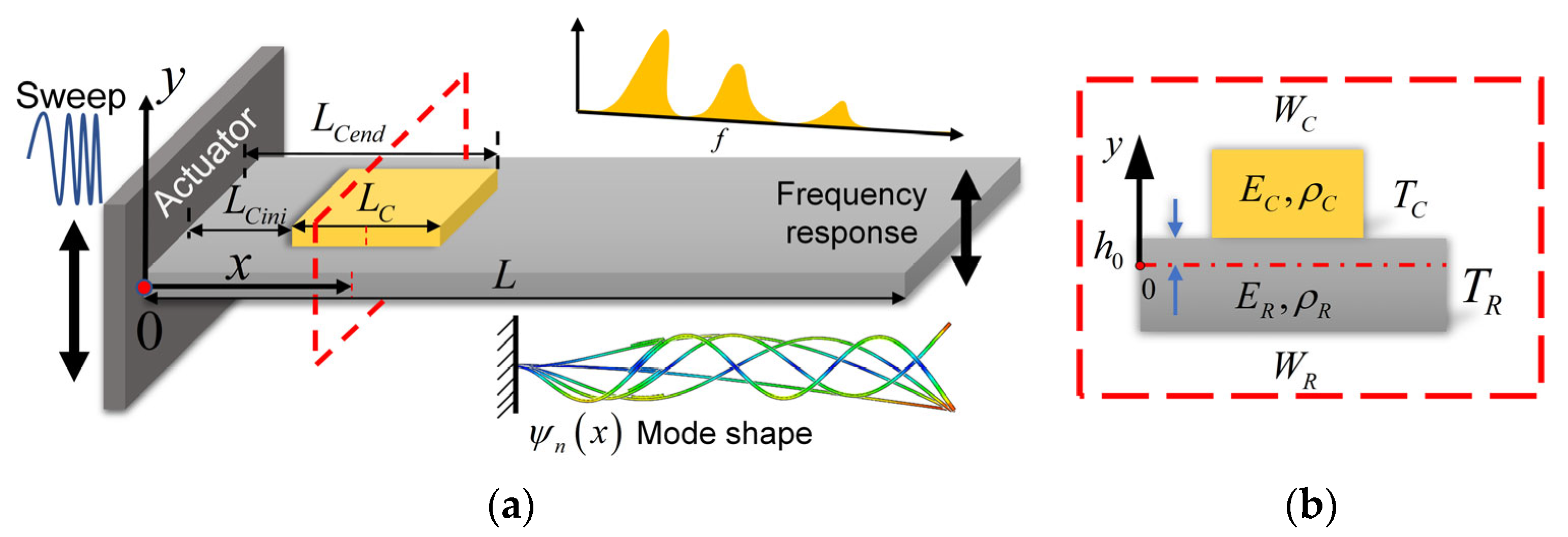
2. Mathematical Modeling

To calculate the Young’s modulus and density of an adsorbate, the first step is to obtain the mode shapes of the resonator. Based on the Euler equation for a beam, the vertical bending vibration of the cantilever resonator can be obtained. The natural frequencies in torsion, lateral bending, and longitudinal vibration modes of the cantilevers are higher than in vertical bending mode, and these mode shapes are more challenging to be measured in the real world than the vertical bending mode shape. To simplify the measurement of vibration frequency and the mathematical calculation, this study focused on the vertical bending vibration modes of the cantilever resonator, thus the vibration modes in torsion, lateral bending, and longitudinal directions are ignored. For simplification and without loss of generality, mode shape changes of the resonator are ignored when the mass and stiffness of the adsorbate are significantly less than that of the resonator [24]. The air-damping effect is complex and unclear [25]. In an atmospheric environment, air damping causes an insignificant effect on the resonator vibration [26]. Furthermore, resonators are commonly applied in vacuum or low atmosphere environments to achieve high-quality factors, which realize high sensitivity and accuracy measurement [27]. So, the damping effect of air is ignored in this study. Materials of both the resonator and the adsorbate are assumed to be linearly elastic, one-layer, and isotropic. Damping, residual stress, and temperature are assumed not to affect the Young’s modulus or density of the resonator and the adsorbate. The minimum dimensions of the mathematical model are larger than the nanoscale. In other words, the mathematical model is based on the assumption that the Young’s modulus and the density of the resonator and the adsorbate are constant. The vertical mode shapes of the cantilever resonator are given as

$${\psi }_n\left(x\right)=A_n\left(\cos {\kappa }_{n}x-\cosh {\kappa }_{n}x\right)+B_n\left(\sin {\kappa }_{n}x-\sinh {\kappa }_{n}x\right)$$

(1)

where ${\psi }_n\left(x\right)$ is the time-independent vibration mode shape of the nth order natural frequency, $x$ is the position along the length of the cantilever from the fixed end. The modal wavenumbers ${\kappa }_n$ are the solutions to $\cos \left({\kappa }_{n}L\right)\cosh \left({\kappa }_{n}L\right)=-1$, and ${\kappa }_{n}L$ = 1.875, 4.694, 7.855, 10.996, 14.137, respectively. $L$ is the length of the cantilever. The mode coefficients fulfill $A_n/B_n=\left(\cos {\kappa }_{n}L+\cosh {\kappa }_{n}L\right)/\left(\sin {\kappa }_{n}L-\sinh {\kappa }_{n}L\right)$ and $A_n/B_n$ = −1.362, −0.982, −1.001, −1.000, −1.000, respectively [5].

In this study, the adsorbate is assumed to be a cuboid. When it is coated on the resonator, it caused both mass and stiffness to increase in the system. The natural frequencies of the vibration system would increase as the stiffness increases and would decrease as the mass increases.

The schematic diagram of the resonator and the adsorbate is shown in Figure 1, where $W_R$, $T_R$, $E_R$, and ${\rho }_R$ are the width, thickness, Young’s modulus, and density parameters of the resonator, respectively. $L_C$, $W_C$, $T_C$, $E_C$ and ${\rho }_C$ are the length, width, thickness, Young’s modulus and density of the adsorbate, respectively. In this study, $E_C$ and ${\rho }_C$ are the parameters that need to be measured. $L_{Cini}$ is the start position of the adsorbate on the cantilever, and $L_{Cend}$ is the end position of the adsorbate on the resonator. $h_0$ is the position of the neutral surface. $y$ is the axis along the thickness direction and the zero point is set on the neutral surface of the section.

Next, the Rayleigh–Ritz method is used to calculate the natural frequencies of the resonator with an adsorbate. The numerator in Equation (2) denotes the total effective stiffness of the resonator and the adsorbate, while the denominator denotes the total effective mass of the resonator and the adsorbate from the fixed end to the free end of the cantilever [18,24].

$${\omega }_n^2=\frac{{\displaystyle {\int }_0^{L_R}D(x)}{\left(\frac{{\partial }^2{\psi }_n(x)}{\partial x^2}\right)}^{2}dx}{{\displaystyle {\int }_0^{L_R}\rho \left(x\right)}{\psi }_n^2(x)dx}$$

(2)

where ${\omega }_n$ is the nth-order angular natural frequency of the vibration system. $D\left(x\right)$ means the bending rigidity of the section. According to the mechanics of materials, the bending rigidity of the resonator section without the adsorbate equals the Young’s modulus of the resonator multiplied by the moment of inertia of the resonator section.

$$D\left(x\right)=E_R\frac{W_R{T}_R^3}{12}\left(0\le x<L_{Cini},L_{Cend}<x\le L\right)$$

(3)

Figure 1b shows the section of the resonator where the adsorbate is located. The position of the neutral surface $h_0$ should be determined first. The position of the neutral surface is found from the condition that the resultant axial force acting on the cross-section is zero [28]. Therefore,

$$E_C{\displaystyle {\int }_{C}ydA}+E_R{\displaystyle {\int }_{R}ydA}=0$$

(4)

In this study, the widths of the adsorbate and the resonator are constant along the length direction of the resonator. So, Equation (4) can be expressed below

$$E_C{W}_C{\displaystyle {\int }_{h_0}^{h_0+T_C}ydy}+E_R{W}_R{\displaystyle {\int }_{h_0-T_R}^{h_0}ydy}=0$$

(5)

Then $h_0$ can be solved as,

$$h_0=\frac{E_R{W}_R{T}_R^2-E_C{W}_C{T}_C^2}{2(E_C{W}_C{T}_C+E_R{W}_R{T}_R)}$$

(6)

The flexural rigidity of the section is expressed as [28]

$$D\left(x\right)=E_C{I}_{C{h}_0}+E_R{I}_{R{h}_0}\left(L_{Cini}\le x\le L_{Cend}\right)$$

(7)

where $I_{C{h}_0}$ and $I_{R{h}_0}$ are the moments of inertia of the adsorbate and resonator. Then $D\left(x\right)$ is expressed as [18]

$$D\left(x\right)=\frac{E_C^2{W}_C^2{T}_C^4+E_R^2{W}_R^2{T}_R^4+E_C{W}_C{T}_C{E}_R{W}_R{T}_R\left(4T_C^2+4T_R^2+6T_C{T}_R\right)}{12\left(E_C{W}_C{T}_C+E_R{W}_R{T}_R\right)}\left(L_{Cini}\le x\le L_{Cend}\right)$$

(8)

$\rho (x)$ means the linear density of the section, presented as

$$\rho \left(x\right)=\{\begin{array}{l}{\rho }_R{W}_R{T}_R\left(0\le x<L_{Cini},L_{Cend}<x\le L\right)\\ {\rho }_R{W}_R{T}_R+{\rho }_C{W}_C{T}_C\left(L_{Cini}\le x\le L_{Cend}\right)\end{array}$$

(9)

Commonly in experiments, the geometry parameters of the resonator and the adsorbate can be measured easily with a scanning electron microscope with nanoscale precision [24]. Resonators are built at nano precision with rigorously selected material, such as high-purity silicon. To calculate the density and Young’s modulus of the adsorbate, it is necessary to obtain the relationship between the Young’s modulus and the density of the adsorbate. Equation (8) contains the relationship between $D\left(x\right)$ and $E_C$. Hence, the next step is to find the relationship between $D\left(x\right)$ and ${\rho }_C$ for different order natural frequencies. Here, Equation (2) is transformed into the following formula.

$$D\left(x\right)=\frac{{\omega }_n^2\left[\left({\rho }_R{W}_R{T}_R\right){\displaystyle {\int }_0^L{\psi }_n^2(x)dx}+{\rho }_C{W}_C{T}_C{\displaystyle {\int }_{L_{Cini}}^{L_{Cend}}{\psi }_n^2(x)}dx\right]-E_R\frac{W_R{T}_R^3}{12}\left[{\displaystyle {\int }_0^{L_{Cini}}{\left(\frac{{\partial }^2{\psi }_n(x)}{\partial x^2}\right)}^2}dx+{\displaystyle {\int }_{L_{Cend}}^L{\left(\frac{{\partial }^2{\psi }_n(x)}{\partial x^2}\right)}^2}dx\right]}{{\displaystyle {\int }_{L_{Cini}}^{L_{Cend}}{\left(\frac{{\partial }^2{\psi }_n(x)}{\partial x^2}\right)}^2}dx}$$

(10)

By combining Equations (8) and (10), the relationship between the density and Young’s modulus of the adsorbate for different order natural frequency is obtained and expressed as

$$E_C=f({\rho }_C,{\omega }_n)$$

(11)

As $E_C$ and ${\rho }_C$ are the material properties of the adsorbate, they should fulfill Equation (11) for different order natural frequencies. The results can be calculated by solving equation sets generated from Equation (11) of different order natural frequency curves. Thus, the determined values of $E_C$ and ${\rho }_C$ can be read out from the intersection of the curves drawn from Equation (11).

3. Results and Discussion

3.1. Numerical Simulation with No Frequency Error

Based on Equation (2) and the parameters in

Table 1. The parameters of the silicon resonator and polymer adsorbate.

Resonator	Material	$L$	$W_R$	$T_R$	$E_R$	${\rho }_R$
	Silicon	400 μm	40 μm	2 μm	168 GPa	2329 kg/m3
Adsorbate	Material	$L_C$	$W_C$	$T_C$	$E_C$	${\rho }_C$
	Polymer	30 μm	30 μm	2 μm	1.36 GPa	746 kg/m3

, a simulation model was built to describe the effect of Young’s modulus and density of the adsorbate on the natural frequencies of the resonator. The geometry and physical parameters of the resonator referred to the size and characteristics of an atomic force microscope silicon cantilever in common usage. The material of the adsorbate referred to the polymer mentioned in Belardinelli’s experiment [24].

Table 2. The natural frequency values when adsorbate located at various positions on the resonator.

${\mathit{L}}_{\mathit{C}\mathit{i}\mathit{n}\mathit{i}}$	0 μm	100 μm	200 μm	370 μm
${\omega }_1 (\mathrm{rad}/\mathrm{s})$	108,892	108,160	107,296	104,421
${\omega }_2 (\mathrm{rad}/\mathrm{s})$	680,706	669,885	668,214	659,332
${\omega }_3 (\mathrm{rad}/\mathrm{s})$	1,901,794	1,863,729	1,889,331	1,847,176
${\omega }_4 (\mathrm{rad}/\mathrm{s})$	3,722,077	3,679,178	3,669,068	3,697,473
${\omega }_5 (\mathrm{rad}/\mathrm{s})$	6,141,323	6,117,132	6,102,113	6,114,159

shows the calculated natural frequencies of the resonator with an adsorbate located at various positions from the fixed end toward the free end of the cantilever. Then the obtained natural frequencies in Table 2 and the parameters in Table 1 except $E_C$ and ${\rho }_C$ were substituted into Equation (11). The Young’s modulus-density curves are shown in Figure 2.

It is noted in Figure 2 that the $E_C$-${\rho }_C$ curves of the first five order natural frequencies intersect at the same point in these figures, and thus the density and Young’s modulus values of the adsorbate can be obtained as $E_C=1.36 \mathrm{GPa}$ and ${\rho }_C=746{ \mathrm{kg}/\mathrm{m}}^3$. The results are consistent with the pre-set ${\rho }_C$ and $E_C$ values in Table 1.

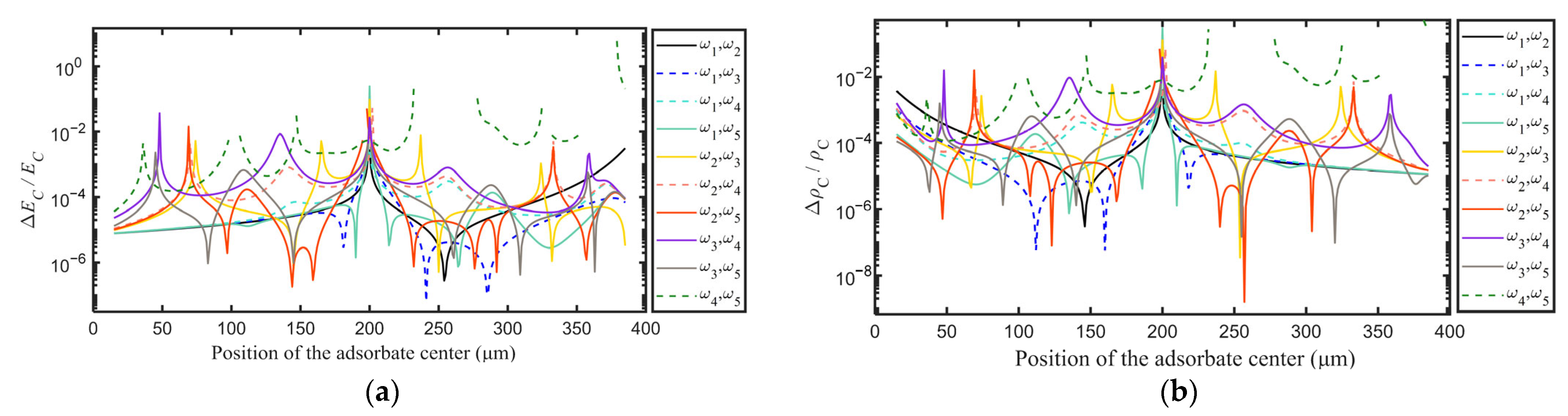
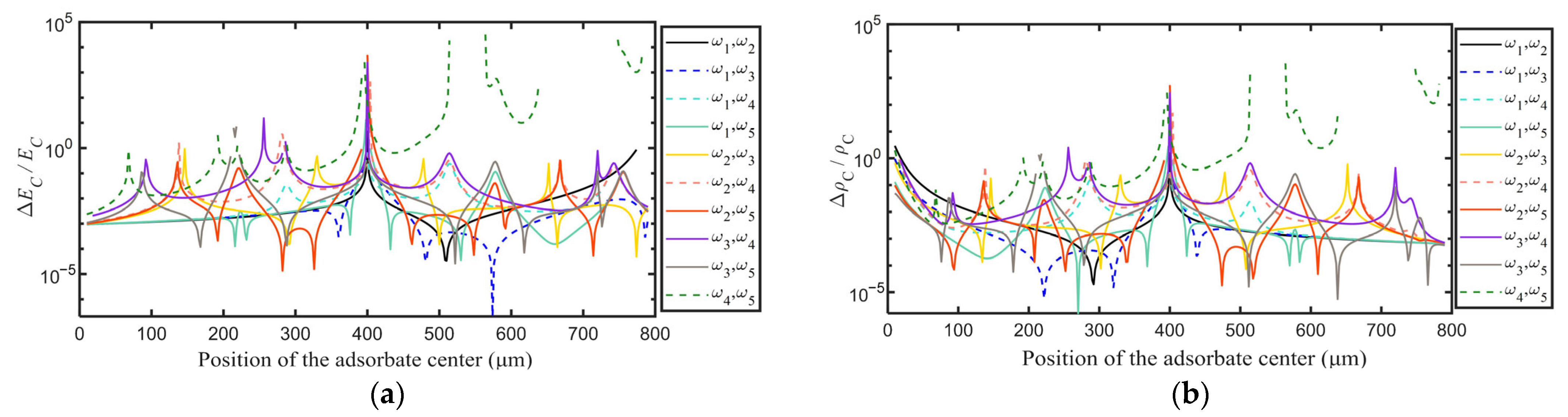
3.2. Analysis of Numerical Simulation Results with Frequency Errors

Errors in the size and material properties are inevitable in the measurement and manufacturing process, which will cause frequency errors in the resonator. So, it is necessary to evaluate how frequency errors affect the calculated $E_C$ and ${\rho }_C$ values. Due to frequency error, the intersections of different order natural frequency $E_C$-${\rho }_C$ curves will not coincide at the same point.

The errors of Young’s modulus values can be presented as $\mathsf{\Delta }{E}_C=|E_{C\left({\omega }_i,{\omega }_j\right)}-E_C|$, in which $E_C=1.36 \mathrm{GPa}$ is the ideal value and $E_{C\left({\omega }_i,{\omega }_j\right)}$ is the Young’s modulus value obtained from the ith and jth order natural frequencies. A relative frequency error of 0.001% was put into each of the first five order natural frequencies. Figure 3a illustrates the relative Young’s modulus errors of the adsorbate calculated from different natural frequency pairs at different positions on the resonator. Similarly, the density error is $\mathsf{\Delta }{\rho }_C=|{\rho }_{C\left({\omega }_i,{\omega }_j\right)}-{\rho }_C|$, in which ${\rho }_C=746{ \mathrm{kg}/\mathrm{m}}^3$ is the ideal value and ${\rho }_{C\left({\omega }_i,{\omega }_j\right)}$ is the density value obtained from the ith and jth order natural frequencies. The relative density errors are shown in Figure 3b. Secondly, the Young’s modulus and density errors caused by 0.01% frequency error are shown in Figure 4a,b.

It can be clearly seen that higher frequency errors will lead to higher Young’s modulus and density errors. Furthermore, by comparing Figure 3a with Figure 4a and Figure 3b with Figure 4b, it is obvious that the curves drawn from different frequency errors show the same trend along the longitude direction. All the peaks in the two relative figures are perfectly located at the same positions. Hence, Figure 3 and Figure 4 proved that the value of the natural frequency error will not change the most appropriate location and frequency pairs for both Young’s modulus and density measurement. It should be noted that some curves appear to be discontinuous in Figure 3 and Figure 4. This is caused by the fact that for specific frequency pairs, their $E_C$-${\rho }_C$ curves did not intersect at the adsorbate positions so there were no available values.

Another simulation with different geometry dimensions of the adsorbate and the resonator was carried out. The material of the adsorbate was set as platinum in this simulation. The parameters of the adsorbate and the resonator are shown in

Table 3. The parameters of the silicon cantilever resonator and platinum adsorbate.

Resonator	Material	$L$	$W_R$	$T_R$	$E_R$	${\rho }_R$
	Silicon	800 μm	40 μm	1 μm	168 GPa	2329 kg/m3
Adsorbate	Material	$L_C$	$W_C$	$T_C$	$E_C$	${\rho }_C$
	Platinum	20 μm	20 μm	1 μm	168 GPa	21,450 kg/m3

.

By comparing Figure 5a with Figure 4a and Figure 5b with Figure 4b, it can be noticed that the curves drawn from different materials or geometry sizes of the adsorbate and resonator show almost the same trend along the longitude direction. For example, the highest peaks all appear at 50% of the length of the cantilever. All the peaks in the two relative figures are perfectly located at the same relative positions. Hence, Figure 4 and Figure 5 proved that the parameters of the adsorbate and resonator do not make a difference to the most appropriate location or frequency pairs for either Young’s modulus or the density measurement.

The numerical simulation results revealed that the measurement accuracy and reliability are affected by the relative position of the adsorbate on the cantilever and the frequency pairs applied. The best frequency pairs for the measurement can be obtained by the following principles. (1) The $\mathsf{\Delta }{E}_C/E_C$ and $\mathsf{\Delta }{\rho }_C/{\rho }_C$ are smallest at the corresponding adsorbate location. This means the calculated Young’s modulus and density are close to the ideal values. (2) The curves change smoothly along the longitudinal axis. As frequency errors are always random, small slopes make the results less sensitive to position errors, as the position is highly related to frequency error.

Based on the principles, the suggestions for Young’s modulus and density measurement are as follows, when the adsorbate is located at a specific position on the resonator, the corresponding best frequency pair for the Young’s modulus measurement can be found in Figure 4a. For example, when the distance between the adsorbate center and the fixed end of the resonator is less than 44% $L$, the results from $\left({\omega }_1,{\omega }_2\right)$, $\left({\omega }_1,{\omega }_3\right)$, and $\left({\omega }_1,{\omega }_5\right)$ change smoothly within a low level. From 56% to 79% $L$, the result from $\left({\omega }_1,{\omega }_3\right)$ appears to be smooth with low error. From 79% $L$ to the free end, $\left({\omega }_1,{\omega }_5\right)$ can provide more accurate results.

As for the measurement of density, the best frequency pair can be found in Figure 4b. From the fixed end to about 23% $L$, $\left({\omega }_1,{\omega }_5\right)$ could provide a better result. From 23% to 35%$L$, $\left({\omega }_1,{\omega }_3\right)$ will be the best choice. Beyond 54% $L$, $\left({\omega }_1,{\omega }_2\right)$, $\left({\omega }_1,{\omega }_3\right)$, and $\left({\omega }_1,{\omega }_5\right)$ can provide good results and their results will get closer as the adsorbate move to the free end of the resonator.

By combining Figure 4a,b, several recommended positions on the resonator and relative natural frequency pairs can be found to measure the density and the Young’s modulus of the adsorbate with good results. The recommended choices are given in

Table 4. Recommended adsorbate center positions and relative natural frequency pairs to measure Young’s modulus and density.

Position	Young’s Modulus	Density
Fixed end-23% $L$	$\left({\omega }_1,{\omega }_2\right)$$,\left({\omega }_1,{\omega }_3\right)$$,\left({\omega }_1,{\omega }_5\right)$	$\left({\omega }_1,{\omega }_5\right)$
23–35% $L$	$\left({\omega }_1,{\omega }_2\right)$$,\left({\omega }_1,{\omega }_3\right)$$,\left({\omega }_1,{\omega }_5\right)$	$\left({\omega }_1,{\omega }_3\right)$
56–79% $L$	$\left({\omega }_1,{\omega }_3\right)$	$\left({\omega }_1,{\omega }_2\right)$$,\left({\omega }_1,{\omega }_3\right)$$,\left({\omega }_1,{\omega }_5\right)$
79% $L$-Free end	$\left({\omega }_1,{\omega }_5\right)$	$\left({\omega }_1,{\omega }_2\right)$$,\left({\omega }_1,{\omega }_3\right)$$,\left({\omega }_1,{\omega }_5\right)$

.

3.3. The Relationship between Error Peaks and the Density to Young’s Modulus Frequency Shift Ratio

To find out what affects the error of density and Young’s modulus measurement of the adsorbate, a simulation was performed and revealed the effects of the density and Young’s modulus on the natural frequencies of the resonator. The result of the polymer adsorbate is shown in Figure 6a. Another simulation result with a platinum adsorbate is shown in Figure 6b.

${\omega }_{{\rho }_n}$ represents the nth order natural frequency of the resonator only affected by the density of the adsorbate, while ${\omega }_{E_n}$ means the nth order natural frequency only affected by the Young’s modulus of the adsorbate. ${\omega }_{Bar{e}_n}$ is the nth-order natural frequency of the cantilever without the adsorbate. $\mathsf{\Delta }{\omega }_{E_n}/\mathsf{\Delta }{\omega }_{{\rho }_n}$ is the ratio of the frequency shift caused by the added Young’s modulus to the frequency shift caused by added density. ${\omega }_{{\rho }_n}$,${\omega }_{E_n}$, and ${\omega }_{Bar{e}_n}$ can be acquired with Equation (2) by using relative parameters.

$$\mathsf{\Delta }{\omega }_{{\rho }_n}/\mathsf{\Delta }{\omega }_{E_n}=\left|{\omega }_{{\rho }_n}-{\omega }_{Bar{e}_n}\right|/\left|{\omega }_{E_n}-{\omega }_{Bar{e}_n}\right|$$

(12)

In Figure 6a, red points are the intersections of different order natural frequency curves. Curves of the fourth and fifth order natural frequencies coincided with each other as the adsorbate moved toward the free end of the resonator.

Interestingly, the horizontal coordinate values of the interactions in Figure 6a matched perfectly with those of the peaks in Figure 4a,b, which means when the adsorbate is located at these positions, the calculated Young’s modulus and density will be inaccurate. Especially for the central point on the resonator, or the middle of the cantilever, all the five order natural frequency curves were almost crossing at the same point in Figure 6a, causing the peaks in Figure 3 and Figure 4 for all different order frequency pairs. Hence, it will be better to locate the adsorbate away from the center of the resonator in the longitudinal direction.

Furthermore, comparing Figure 6a with Figure 6b, the geometry parameters and mechanical properties of the adsorbate and resonator mainly influence the amplitude of the plots in Figure 6a but hardly affect the trend of the plots and the positions of the interactions. As a result, the suggestions provided for the choice of adsorbate position and frequency pair are capable of measuring adsorbates with different materials and different dimensions.

4. Measurement Procedures and Finite Element Analysis Simulation Validation

The detailed procedures to measure Young’s modulus and density of the adsorbate on a cantilever in a real-world application are listed as follows.

4.1. The Procedures of Young’s Modulus and Density Measurement

• Firstly, prepare a large length-to-thickness ratio rectangle cantilever resonator with known Young’s modulus and density values.
• Place the adsorbate that needs to be measured on one surface of the cantilever resonator. The adsorbate should be securely fixed to the cantilever so it will not separate or change its location during frequency measurement. Commonly, the fixed end of the cantilever is better for Young’s modulus measurement, while the free end of the resonator performs better for density measurement. Furthermore, avoid putting the adsorbate in the center of the longitudinal direction of the cantilever.
• Measure the geometry parameters of the resonator and the adsorbate, including the length, width, thickness, and relative position in a scanning electron microscope.
• Measure the vertical bending mode natural frequencies of the cantilever and the adsorbate with a contactless method. The measurement device can be atomic force microscopy or a laser doppler vibrometer.
• Find the best frequency pairs for the Young’s modulus and density measurement from Table 4 according to the relative position of the adsorbate measured in step 3.
• Input the length, width, and thickness of the adsorbate and the resonator, the location of the adsorbate center on the resonator, the first five order natural frequencies, and the Young’s modulus and density of the cantilever into Equation (11) to plot the Young’s modulus and density curves of the adsorbate for different order natural frequencies. The interaction of the frequency pairs chosen in step 5 will be the determined Young’s modulus and density.

In real-world applications, air damping will decrease the natural frequencies of the cantilever. The best way is to carry out the experiment in a vacuum. If not, it is better to measure the natural frequency of the cantilever without the adsorbate in the air to evaluate the effect of the air damping. The residual stress in the microcantilever may make the mode shape of the cantilever different from the theoretical result and affect the measurement accuracy. It is recommended to use the resonator after its residual stress has been released. Temperature may affect the mechanical properties of the cantilever and the adsorbate. It may cause residual stress between the adsorbate and resonator, and change the density, and the stiffness. Therefore, keeping the temperature stable during the experiment would help to improve the measurement accuracy and reliability.

To validate the proposed method, an FEA model was applied in this research.

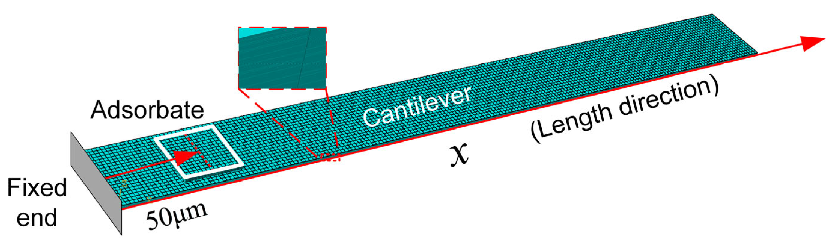
4.2. Finite Element Analysis Validation

The parameters of the adsorbate and resonator were set according to Table 1. The length, width, and thickness of the cantilever were 400 μm, 40 μm, and 2 μm, respectively. The length, width, and thickness of the adsorbate were 30 μm, 30 μm, and 2 μm, respectively. The Poisson’s ratio of them was set as 0. The interface between the adsorbate and the resonator was constrained as a Tie type in Abaqus software. The fixed-end surface of the cantilever was constrained with no displacement in any direction. The center of the adsorbate was located at 50 μm from the fixed end of the cantilever. The mesh element shape was Hexahedron. The FEA model is shown in Figure 7.

The first five order vertical bending angular natural frequencies and relative mode shapes simulated with the FEA method are shown in Figure 8.

Putting these bending natural frequencies into Equation (11), the Young’s modulus and density of the adsorbate were calculated from each frequency pair, as shown in

Table 5. The Young’s modulus and density calculated from different natural frequency pairs.

Parameters	$\left({\omega }_1,{\omega }_2\right)$	$\left({\omega }_1,{\omega }_3\right)$	$\left({\omega }_1,{\omega }_4\right)$	$\left({\omega }_1,{\omega }_5\right)$	$\left({\omega }_2,{\omega }_3\right)$
$E_C$ (GPa)	1.309	1.037	1.306	1.306	1.087
${\rho }_C$ (kg/m3)	1180	862.2	775.0	760.5	853.4
Parameters	$\left({\omega }_2,{\omega }_4\right)$	$\left({\omega }_2,{\omega }_5\right)$	$\left({\omega }_3,{\omega }_4\right)$	$\left({\omega }_3,{\omega }_5\right)$	$\left({\omega }_4,{\omega }_5\right)$
$E_C$ (GPa)	1.022	1.003	5.502	2.918	1.650
${\rho }_C$ (kg/m3)	757.7	729.0	1027	926.0	795.9

.

Based on the curves in Figure 9a, the $\mathsf{\Delta }{E}_C/E_C$ values calculated from $\left({\omega }_1,{\omega }_2\right)$, $\left({\omega }_1,{\omega }_3\right)$, $\left({\omega }_1,{\omega }_4\right)$, and $\left({\omega }_1,{\omega }_5\right)$ are relatively lower than other frequency pairs at the 50 μm position. As for the $\mathsf{\Delta }{\rho }_C/{\rho }_C$ curves of different frequency pairs shown in Figure 9b, $\left({\omega }_1,{\omega }_5\right)$ and $\left({\omega }_2,{\omega }_5\right)$ can provide better results at this location. However, the curves of $\left({\omega }_1,{\omega }_5\right)$ changed more gently without sudden change, making the calculated result less sensitive, so the result from this frequency pair will be more stable and reliable. Additionally, these frequency pairs coincided with the recommended frequency pairs mentioned in Table 3.

Finally, $\left({\omega }_1,{\omega }_2\right)$ was picked out for the Young’s modulus measurement and $\left({\omega }_1,{\omega }_5\right)$ was picked out for the density measurement of the adsorbate. The $E_C$ was calculated as 1.309 GPa, with an error of 3.75% compared with the ideal value of 1.36 GPa. Furthermore, the ${\rho }_C$ was calculated as 760.5 kg/m³, with an error of −1.94% compared with the ideal density value of 746 kg/m³. The selected frequency pairs and the relative Young’s modulus and density result are shown in Figure 10.

5. Conclusions

In summary, a mathematical model based on the Rayleigh–Ritz method was built to determine the Young’s modulus and density of an adsorbate by measuring several vertical vibration natural frequencies of the resonator and extracting the intersections of their nonlinear Young’s modulus and density curves. Ideally, the intersections of different natural frequency curves would coincide, which revealed the Young’s modulus and density of the adsorbate simultaneously. This research revealed a vital conclusion, that when there were errors in the measurement of natural frequencies, the position of the adsorbate had a complicated and nonlinear effect on the measurement accuracy of Young’s modulus and density. Furthermore, this study revealed that frequency pairs and the relative position of the adsorbate on the cantilever are two important factors that affect the accuracy and reliability of the measurement. Using appropriate frequency pairs can improve the accuracy and reliability of measurement. This study provided a method to set the adsorbate at specific positions and choose suitable natural frequency pairs to obtain more accurate and stable results. Finally, the method was validated by the finite element analysis method.

The results from this study show the potential application of combining several high-order natural frequencies to improve measurement accuracy. It can be applied in real-time micro/nano-scale research and provide researchers with intensive data to monitor the mechanical properties variation in the experimental process. It is a non-invasive and label-free scheme that works to monitor the biological reaction or to distinguish the cell by its mechanical properties without destroying the sample.

References

1. Johnson, B.N.; Mutharasan, R. Biosensing using dynamic-mode cantilever sensors: A review. Biosens. Bioelectron. 2012, 32, 1–18. [Google Scholar] [CrossRef] [PubMed]
2. Wang, K.; Wang, B. Vibration modeling of carbon-nanotube-based biosensors incorporating thermal and nonlocal effects. J. Vib. Control. 2014, 22, 1405–1414. [Google Scholar] [CrossRef]
3. Dohn, S.; Schmid, S.; Amiot, F.; Boisen, A. Position and mass determination of multiple particles using cantilever based mass sensors. Appl. Phys. Lett. 2010, 97, 044103. [Google Scholar] [CrossRef]
4. Ekinci, K.L.; Huang, X.M.H.; Roukes, M.L. Ultrasensitive nanoelectromechanical mass detection. Appl. Phys. Lett. 2004, 84, 4469–4471. [Google Scholar] [CrossRef] [Green Version]
5. Dohn, S.; Svendsen, W.; Boisen, A.; Hansen, O. Mass and position determination of attached particles on cantilever based mass sensors. Rev. Sci. Instrum. 2007, 78, 103303. [Google Scholar] [CrossRef] [Green Version]
6. Sader, J.E.; Hanay, M.S.; Neumann, A.P.; Roukes, M.L. Mass Spectrometry Using Nanomechanical Systems: Beyond the Point-Mass Approximation. Nano Lett. 2018, 18, 1608–1614. [Google Scholar] [CrossRef] [Green Version]
7. Yuksel, M.; Orhan, E.; Yanik, C.; Ari, A.B.; Demir, A.; Hanay, M.S. Nonlinear Nanomechanical Mass Spectrometry at the Single-Nanoparticle Level. Nano Lett. 2019, 19, 3583–3589. [Google Scholar] [CrossRef] [Green Version]
8. Tsai, T.-T.; Fang, Y.-C.; Wu, S.-K.; Chang, R.-H.; Chien, W.-C.; Chang, Y.-H.; Wu, C.-S.; Kuo, W. High throughput and label-free particle sensor based on microwave resonators. Sens. Actuators A Phys. 2019, 285, 652–658. [Google Scholar] [CrossRef]
9. Fritz, J.; Baller, M.K.; Lang, H.P.; Rothuizen, H.; Vettiger, P.; Meyer, E.; Guntherodt, H.; Gerber, C.; Gimzewski, J.K. Translating biomolecular recognition into nanomechanics. Science 2000, 288, 316–318. [Google Scholar] [CrossRef] [Green Version]
10. Majstrzyk, W.; Mognaschi, M.E.; Orłowska, K.; di Barba, P.; Sierakowski, A.; Dobrowolski, R.; Grabiec, P.; Gotszalk, T. Electromagnetic cantilever reference for the calibration of optical nanodisplacement systems. Sens. Actuators A Phys. 2018, 2018, 149–156. [Google Scholar] [CrossRef]
11. Chen, F.; Gao, J.; Tian, W. Force-frequency characteristics of multi-electrode quartz crystal resonator cluster. Sens. Actuators A Phys. 2018, 269, 427–434. [Google Scholar] [CrossRef]
12. Ekmekci, E.; Kose, U.; Cinar, A.; Ertan, O.; Ekmekci, Z. The use of metamaterial type double-sided resonator structures in humidity and concentration sensing applications. Sens. Actuators A Phys. 2019, 297, 111559. [Google Scholar] [CrossRef]
13. Laidoudi, F.; Kanouni, F.; Assali, A.; Caliendo, C.; Amara, S.; Nezzari, H.; Boubenider, F. Thickness shear SMR resonator based on Yttrium-doped AlN for high sensitive liquid sensors. Sens. Actuators A Phys. 2021, 333, 113238. [Google Scholar] [CrossRef]
14. Eom, K.; Park, H.S.; Yoon, D.S.; Kwon, T. Nanomechanical resonators and their applications in biological/chemical detection: Nanomechanics principles. Phys. Rep. 2011, 503, 115–163. [Google Scholar] [CrossRef] [Green Version]
15. Parmar, J.; Patel, S.K. Tunable and highly sensitive graphene-based biosensor with circle/split ring resonator metasurface for sensing hemoglobin/urine biomolecules. Phys. B Condens. Matter 2022, 624, 413399. [Google Scholar] [CrossRef]
16. Suresh, S. Biomechanics and biophysics of cancer cells. Acta Biomater. 2007, 3, 413–438. [Google Scholar] [CrossRef] [PubMed]
17. Garcia, R.; Herruzo, E.T. The emergence of multifrequency force microscopy. Nat. Nanotechnol. 2012, 7, 217–226. [Google Scholar] [CrossRef] [Green Version]
18. Ramos, D.; Tamayo, J.; Mertens, J.; Calleja, M.; Villanueva, L.G.; Zaballos, A. Detection of bacteria based on the thermomechanical noise of a nanomechanical resonator: Origin of the response and detection limits. Nanotechnology 2008, 19, 035503. [Google Scholar] [CrossRef]
19. Calleja, M.; Kosaka, P.M.; San Paulo, A.; Tamayo, J. Challenges for nanomechanical sensors in biological detection. Nanoscale 2012, 4, 4925–4938. [Google Scholar] [CrossRef] [Green Version]
20. Teva, J.; Abadal, G.; Torres, F.; Verd, J.; Perez-Murano, F.; Barniol, N. A femtogram resolution mass sensor platform based on SOI electrostatically driven resonant cantilever. Part II: Sensor calibration and glycerine evaporation rate measurement. Ultramicroscopy 2006, 106, 808–914. [Google Scholar] [CrossRef]
21. Jensen, K.; Kim, K.; Zettl, A. An atomic-resolution nanomechanical mass sensor. Nat. Nanotechnol. 2008, 3, 533–537. [Google Scholar] [CrossRef] [PubMed]
22. Lassagne, B.; Garcia-Sanchez, D.; Aguasca, A.; Bachtold, A. Ultrasensitive mass sensing with a nanotube electromechanical resonator. Nano Lett. 2008, 8, 3735–3738. [Google Scholar] [CrossRef] [PubMed]
23. Gil-Santos, E.; Ramos, D.; Martinez, J.; Fernandez-Regulez, M.; Garcia, R.; San Paulo, A.; Calleja, M.; Tamayo, J. Nanomechanical mass sensing and stiffness spectrometry based on two-dimensional vibrations of resonant nanowires. Nat. Nanotechnol. 2010, 5, 641–645. [Google Scholar] [CrossRef] [PubMed] [Green Version]
24. Belardinelli, P.; Hauzer, L.M.F.R.; Šiškins, M.; Ghatkesar, M.K.; Alijani, F. Modal analysis for density and anisotropic elasticity identification of adsorbates on microcantilevers. Appl. Phys. Lett. 2018, 113, 143102. [Google Scholar] [CrossRef] [Green Version]
25. Lavrik, N.V.; Sepaniak, M.J.; Datskos, P.G. Cantilever transducers as a platform for chemical and biological sensors. Rev. Sci. Instrum. 2004, 75, 2229–2253. [Google Scholar] [CrossRef]
26. Zhang, Y. Detecting the stiffness and mass of biochemical adsorbates by a resonator sensor. Sens. Actuators B Chem. 2014, 202, 286–293. [Google Scholar] [CrossRef]
27. Keeler, E.G.; Jing, P.; Wu, J.; Zou, C.; Lin, L.Y. MEMS Resonant Mass Sensor With Integrated Optical Manipulation. IEEE Trans. Nanotechnol. 2018, 17, 714–718. [Google Scholar] [CrossRef]
28. Goodno, B.J.; Gere, J.M. Mechanics of Materials, 9th ed.; Cengage Learning: South Melbourne, VIC, Australia, 2018; pp. 553–637. [Google Scholar]
Figure 1. (a) The schematic diagram of the cantilever resonator with an adsorbate. (b) The cross-section of the adsorbate and the resonator.
Actuators 11 00335 g001
Figure 2. The first five order natural frequency E C - ρ C curves. The red points denote the ideal Young’s modulus and density values of the adsorbate. The left side of the adsorbate L C i n i on the resonator was: (a) the fixed end. (b) 100 μm from the fixed end. (c) 200 μm from the fixed end. (d) the free end.
Actuators 11 00335 g002
Figure 3. The relative physical parameter errors of the polymer adsorbate when 0.001% frequency error were added to the first five order natural frequencies. (a) Young’s modulus errors, (b) Density errors.
Actuators 11 00335 g003
Figure 4. The relative physical parameter errors of the polymer adsorbate when 0.01% frequency error were added to the first five order natural frequencies. (a) Young’s modulus errors, (b) Density errors.
Actuators 11 00335 g004
Figure 5. The relative physical parameter errors of the platinum adsorbate when 0.01% frequency error were added to the first five order natural frequencies. (a) Young’s modulus errors, (b) Density errors.
Actuators 11 00335 g005
Figure 6. The ratio of the frequency shift caused by added density to the frequency shift caused by added Young’s modulus. (a) The curves are simulated with parameters in Table 1, the material of the adsorbate is polymer (b) The curves are simulated with parameters in Table 3, the material of the adsorbate is platinum.
Actuators 11 00335 g006
Figure 7. The FEA model of the cantilever resonator and adsorbate.
Actuators 11 00335 g007
Figure 8. The first five order bending angular natural frequencies and relative mode shapes.
Actuators 11 00335 g008
Figure 9. The partial zoom of Figure 4 contains the curves of different frequency pairs of the adsorbate locating at 50 μm from the fixed end of the resonator. (a) Young’s modulus errors, (b) Density errors.
Actuators 11 00335 g009
Figure 10. E C - ρ C curves of the first five order natural frequencies and the recommended frequency pairs to calculate the Young’s modulus and density values of the adsorbate.
Actuators 11 00335 g010