Article

Adaptive Robust Tracking Control for Near Space Vehicles with Multi-Source Disturbances and Input–Output Constraints

1
Key Laboratory of Applied Mathematics and Artificial Intelligence Mechanism, Hefei University, Hefei 230601, China
2
School of Mechanical and Electrical Engineering, Zaozhuang University, Zaozhuang 277160, China
3
Huawei Technologies Co., Ltd., Shenzhen 518129, China
*
Author to whom correspondence should be addressed.
Actuators 2022, 11(10), 273; https://doi.org/10.3390/act11100273
Submission received: 29 August 2022 / Revised: 14 September 2022 / Accepted: 20 September 2022 / Published: 23 September 2022
(This article belongs to the Special Issue Intelligent Control of Flexible Manipulator Systems and Robotics)

Abstract

:
In this paper, considering the simultaneous influence of multi-source disturbances, system modeling uncertainties and input–output constraints, an adaptive robust attitude tracking control scheme is proposed for near space vehicles (NSVs) which is expressed as a stochastic nonlinear system. A multi-dimensional Taylor polynomial network (MTPN) is utilized to handle the system uncertainties, and the nonlinear disturbance observer (NDO) based on MTPN is designed to estimate the external disturbances. Furthermore, by constructing the auxiliary system to tackle the input saturation and introducing the Tan-type barrier Lyapunov function (TBLF) to solve the output constraint, the constrained control strategy can be obtained. Combining with backstepping control (BC) technique and stochastic control method, an adaptive robust stochastic control scheme is developed based on NDO, MTPN, and auxiliary system, and the closed-loop system stability in the sense of probability is analyzed based on stochastic Lyapunov stability theory. Finally, numerical simulations further demonstrate the feasibility of the proposed tracking control scheme.

1. Introduction

Near space generally refers to the airspace between 20 km and 100 km above the surface. As a new space for military science and technology applications, near space has very important application and development value and far-reaching strategic significance. As the focus of international space technology, near space vehicle (NSV) is an aircraft that can continuously work in near space to perform some predefined tasks. It has the characteristics of strong survivability, strong mobility, reusability and wide coverage. The research and development of NSV is not only the embodiment of national comprehensive strength, but also the guarantee for the rational use of near space resources to ensure national security [1]. In order to improve the flight performance and the ability to carry out the given tasks, many advanced control theories and methods have been applied to the design of flight control systems, and the satisfactory flight control performance has been achieved, such as sliding mode control [2,3,4], H control [5], robust adaptive control [6,7,8,9,10] and so on.
In all the actual control systems, there exist various forms of disturbances, which will not only affect the control performance of the system, but even cause the instability of the whole control system. As such, the research on disturbance suppression in control system design has always been particularly important [11]. In order to solve the disturbance suppression problem of the control system with unmeasurable disturbance, many different types of disturbance observer (DO) with the help of the known information of the control system were designed [12,13,14,15,16]. The output of DO is used to compensate for the influence of disturbance on the control system, and the ideal control effect can be achieved. Therefore, the control method based on DO can be well applied to study the anti-disturbance control of aircraft. In [12], a robust control scheme based on the nonlinear DO and dynamic inverse method was proposed for the missile longitudinal control system. In [13], the output feedback controller of hypersonic vehicle was designed by combining the neural network and high gain DO. In [14], a robust flight control scheme based on DO was proposed to realize the longitudinal dynamic control of hypersonic vehicle with mismatched disturbance. A novel adaptive neural network control scheme based on the sliding mode DO was proposed in [15]. In [16], the coupling effect caused by wind was regarded as an unknown disturbance, and an adaptive neural control strategy based on DO was designed. However, when the uncertain external disturbance exists in the control input channel, the control method is relatively conservative, which can only attenuate the disturbance and cannot effectively offset the influence of the external disturbance. In order to better handle this problem, a hybrid H 2 / H robust fuzzy controller based on disturbance observer was designed in [17], and combined with disturbance observer technology to realize longitudinal tracking control of hypersonic vehicle.
With the increasingly high requirements for the control system, it is necessary to take into account some different types of external disturbances, such as the external environment noise and the measurement noise of the system, external time-varying disturbance and so on to improve the robustness of the NSV flight control system. In the field of flight control, some stochastic control methods have also been studied [7,18,19,20,21]. For example, a stochastic optimal sliding mode control scheme was proposed in [18], which can realize active control of flexible aircraft. A robust stochastic control scheme based on state observer was proposed in [19] and applied to the flight control system. In [20], a robust attitude motion stabilization controller was designed by using a geometric stochastic feedback control method for rigid body aircraft with random input torque. In [21], a fuzzy adaptive robust stochastic control scheme was proposed for the multiple input multiple output stochastic Poisson jump diffusion system with continuous and discontinuous random fluctuations, and the control strategy was applied to the trajectory tracking control of four rotor aircraft.
From another perspective, the practical engineering systems need to meet many constraint requirements, which also means that the constrained control problems have obtained a lot of attention and research. In [22], the state constraints problem was studied, and a finite-time adaptive fuzzy control scheme was developed for hypersonic vehicles. By constructing an auxiliary system to tackle the input saturation, an adaptive fault-tolerant control strategy based on the composite DO and neural networks was proposed in [23]. In [24], by introducing the smooth nonlinear function based on Sigmoid function to approximate the input saturation function, a robust constrained control scheme based on fuzzy logic systems and high-order DO was presented for a class of uncertain nonlinear systems. In [25], based on DO and neural networks, an adaptive discrete-time fractional-order controller was designed with prescribed performance for UAV with external disturbances and input constraints. In [26], a robust adaptive boundary control based on neural network was proposed for flexible manipulator with uncertainties and input saturation. In order to handle the output constraint problem, on the basis of a barrier Lyapunov function, an adaptive neural network control scheme was proposed for the helicopter system with hysteresis in [27]. However, considering the simultaneous influence of multi-source disturbances, system modeling uncertainties and input–output constraints, the research on flight control technology for NSV is relatively less developed. Therefore, the robust anti-disturbance constrained flight control problem of NSV needs to be further studied.
Motivated by the above analysis, we consider the simultaneous influence of multi-source disturbances, system modeling uncertainties and input–output constraints acting on the NSV attitude control system in this paper. The attitude tracking control problem is studied and an adaptive robust stochastic control scheme is proposed based on MTPN, disturbance observer and auxiliary system. The main contributions of this manuscript are as follows:
(1)
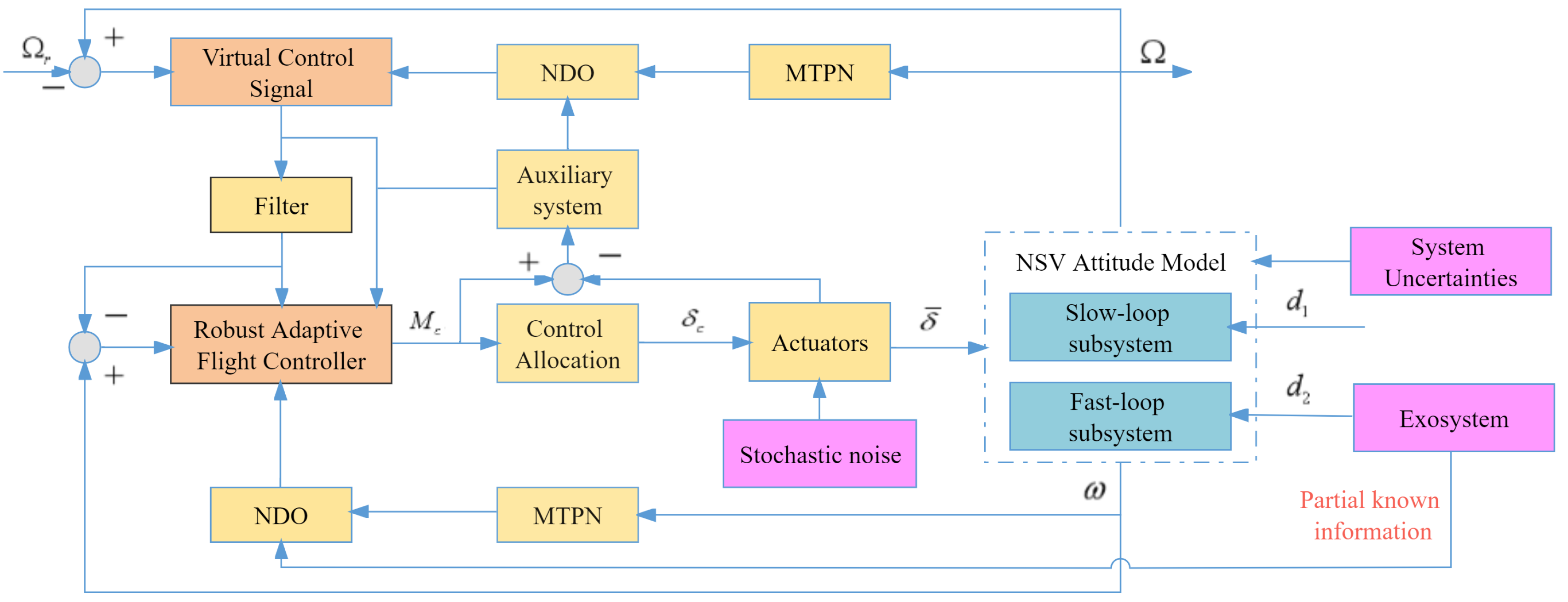
Considering the simultaneous influence of multi-source disturbances, system modeling uncertainties and input–output constraints acting on the NSV attitude control system, and according to stochastic theory, a novel attitude motion dynamic of the NSVs is modeled as the MIMO stochastic nonlinear system.
(2)
To improve the control time-effectiveness, MTPN is utilized to handle the system uncertainties. The interactive design is realized by incorporating MTPN and DO, and a nonlinear DO based on MTPN is designed to estimate the external time-varying disturbances.
(3)
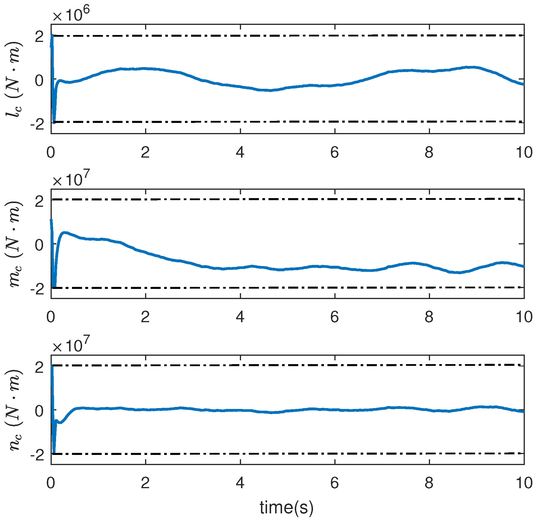
By constructing the auxiliary system to tackle the input saturation and introducing TBLF to solve the output constraint, the constrained control strategy can be obtained. The adaptive robust stochastic control scheme is developed based on NDO, MTPN, and auxiliary system, and the closed-loop system stability in the sense of probability is analyzed based on stochastic Lyapunov stability theory.
The rest of this paper is organized according to the following framework. Section 2 and Section 3 present the preliminaries and problem formulation, respectively. The robust constrained controller design and stability analysis are given in Section 4. Section 5 provides the simulation results. Finally, the conclusions are given in Section 6.

2. Preliminaries

Consider the following I t o ^ type stochastic differential equation (SDE) [28]:
d x = f ( x ) d t + g ( x ) d w , x ( 0 ) = x 0 R n ,
where x R n is the system state vector, and w denotes the appropriate dimensional standard wiener process defined in complete probability space. The nonlinear functions f ( x ) : R n R n and g ( x ) : R n R n × m are Borel measurable functions and satisfy the local Lipschitz condition with respect to x.
Definition 1
([28]). For any given twice continuously differentiable function V C 2 ( R n , R ) , the infinite differential operator along with SDE (1) is defined as the following form:
L V = V x f ( x ) + 1 2 t r { g T ( x ) 2 V x 2 g ( x ) }
where t r { · } denotes the trace of a matrix.
Lemma 1
([7]). Consider the stochastic nonlinear system (1), if there exists a positive definite, radially unbounded, twice continuously differentiable Lyapunov function V : R n R + and constants a 0 > 0 , b 0 0 such that
L V ( x ) a 0 V ( x ) + b 0
then (i) the system has a unique solution almost surely, and (ii) the system is bounded in probability.
Because of the strong approximation ability, neural networks are often used to deal with system uncertainties, and many adaptive neural network control schemes were developed. Meanwhile, as a network structure, a multi-dimensional Taylor polynomial network (MTPN) is composed with multivariable polynomials [29,30]. It has the characteristics of simple structure, strong learning ability and adaptability, which is advantageous to improve the control time-effectiveness. The typical expression is as follows:
f ^ ( z ) = W T P m ( z )
where z = [ z 1 , , z n ¯ ] T R n ¯ is the network input of MTPN, and W = [ w 1 , , w l ] T R l is the weight vector of the MTPN. P m ( z ) denotes the basis vector function, and the element of P m ( z ) is expressed as i , j = 1 n ¯ z i n i z j n j , where n i 0 , n j 0 satisfying 0 n i + n j m .
Lemma 2
([29]). Suppose that f ( z ) is a continuous function defined in the compact set Θ R n . For any given positive constant ε ¯ > 0 , there exists an MTPN W T P m ( z ) such that
f ( z ) = W T P m ( z ) + ϵ ( z ) , | ϵ ( z ) | ε ¯
where ϵ ( z ) is the approximation error vector.
Lemma 3
([31]). (Young Inequality) For any x ¯ , y ¯ R and positive constant > 0 , there exist constants > 1 and > 1 with ( 1 ) ( 1 ) = 1 , such that the following inequality holds:
x ¯ y ¯ | x ¯ | + 1 | y ¯ |

3. Problem Formulation

In [7], considering the stochastic noise disturbances acting on the control input channel, and the attitude model of the NSV system is described in the following form:
d Ω = ( F 1 ( Ω ) + G 1 ( Ω ) ω + Δ F 1 ) d t d ω = ( F 2 ( Ω , ω ) + G 2 ( Ω , ω ) s a t ( u ) + Δ F 2 ) d t + G 2 ( Ω , ω ) G δ Σ d w y = Ω
where Ω = [ α , β , μ ] T and ω = [ p , q , r ] T are the attitude angle and angular rate, respectively. F 1 and F 2 are known nonlinear system functions. G 1 and G 2 are known control gain matrices. Δ F 1 = [ Δ f 11 , Δ f 12 , Δ f 13 ] T and Δ F 2 = [ Δ f 21 , Δ f 22 , Δ f 23 ] T denote the unknown nonlinear smoothly functions which are system uncertainties caused by the modeling error; s a t ( u ) = [ s a t ( u 1 ) , s a t ( u 2 ) , s a t ( u 3 ) ] T is the saturation control input with s a t ( · ) being defined as follows:
s a t ( u i ) = u ¯ i M s i g n ( u i ) , | u i | u ¯ i M u i , | u i | < u ¯ i M
where u ¯ i M is the known bound of the saturation control input. In view of the limited space, the detailed definitions of variables, aerodynamic parameters and relevant system functions can be found in [7,32].
In this paper, further consider the influence of multi-source disturbances and input–output constraints acting on the NSV attitude control system in the actual flight process, and denoting x 1 = Ω ,   x 2 = ω ,   x ¯ 2 = [ Ω T ,   ω T ] T , H = G 2 G δ . The NSV attitude dynamics model can be further rewritten under the formula:
d x 1 = ( F 1 ( x 1 ) + G 1 ( x 1 ) x 2 + Δ F 1 ( x 1 ) + d 1 ( t ) ) d t d x 2 = ( F 2 ( x ¯ 2 ) + G 2 ( x ¯ 2 ) s a t ( u ) + Δ F 2 ( x ¯ 2 ) + d 2 ( t ) ) d t + H Σ d w y = x 1
where d 1 ( t ) denotes the external time-varying disturbance, and d 2 ( t ) denotes the external disturbance with partial known information.
To facilitate the attitude tracking controller design of the system (9), the following assumptions need to be given:
Assumption 1.
The external time-varying disturbance d 1 is piecewise smooth and bounded; that is, there exist positive constants d ˇ 1 > 0 and d ¯ 1 > 0 , such that d 1 d ˇ 1 and d ˙ 1 d ¯ 1 .
Assumption 2.
Considering that the partial information of the external disturbance d 2 = [ d 21 , d 22 , d 23 ] T is known, it always is assumed that the external disturbance d 2 i ( i = 1 , 2 , 3 ) is generated by the following exosystem:
ϖ ˙ i = M i ϖ i + N i ξ ¯ i , d 2 i = L i ϖ i
where the intermediate variable ϖ i is the system vector of the exosystem, ξ ¯ i denotes a Gaussian white noise vector, M i ,   N i and L i are known constant matrices.
Remark 1.
In practical engineering systems, a large number of external disturbances have inherent characteristics such as harmonic and unknown constant load, and can be regarded as being generated by a neutral and stable external interference model (10). According to the different cases of the system state matrices, different types of external disturbances can be obtained and listed as follows.
(1)
When M i = 0 ,   L i = 1 ,   N i = 0 , d 2 i is an unknown constant disturbance.
(2)
When M i = 0 2.5 2.5 0 , N i = 0 0 0 0 , L i = [ 0 , 3 ] , d 2 i is an harmonic disturbance with known frequencies as shown in Figure 1a.
(3)
When M i = 0 2.5 2.5 0 , N i = 2 0 0 2 , L i = [ 2 , 0 ] , d 2 i is a external disturbance with random excitation term as shown in Figure 1b.
Assumption 3.
According to controllability and safety of the actual flight, the intensity of white noises σ i ,   i = 1 , 2 , 3 are considered to be finite. Furthermore, the matrix Σ is norm bounded, and there exists a positive constant σ ¯ > 0 such that Σ 2 σ ¯ .
Assumption 4.
For the NSV attitude nonlinear system (9) with multiple disturbances, G 1 and G 2 are invertible and norm bounded, i.e., G j g j * ,   j = 1 , 2 , where g j * > 0 are unknown positive constants.
Assumption 5.
The output constraint signal k d ( t ) and the expected reference signal y r are second-order derivable, and their respective derivatives are bounded.
According to Assumption 2, and combining with stochastic system theory by taking d w ¯ i d t instead of ξ ¯ i , where w ¯ i denotes a standard wiener process. Therefore, the NSV attitude nonlinear system (9) can be rewritten to the following MIMO stochastic nonlinear system:
d x 1 = ( F 1 + G 1 x 2 + Δ F 1 + d 1 ) d t d x 2 = ( F 2 + G 2 s a t ( u ) + Δ F 2 + d 2 ) d t + H Σ d w y = x 1
d ϖ = M ϖ d t + N d w ¯ , d 2 = L ϖ
where ϖ = [ ϖ 1 T , ϖ 2 T , ϖ 3 T ] T is the state vector of the exosystem; w ¯ = [ w ¯ 1 T , w ¯ 2 T , w ¯ 3 T ] T , M = d i a g { M 1 , M 2 , M 3 } , N = d i a g { N 1 , N 2 , N 3 } , L = d i a g { L 1 , L 2 , L 3 } .
In this paper, our main goal is to design an adaptive robust constrained tracking control strategy for the NSV system models (11) and (12) based on NDO, auxiliary system and TBLF. The proposed scheme can guarantee that the system output y can track the desired reference signal y r , and meets the constraint requirements of tracking error. Moreover, all the signals of the closed-loop system are semi-globally uniform and ultimately bounded in the probability sense. The adaptive robust control structural diagram is shown in Figure 2.

4. Adaptive Robust Stochastic Controller Design Based on NDO and TBLF

4.1. Adaptive Constrained Controller Design

In this section, an adaptive robust stochastic control scheme based on NDO, MTPN and auxiliary system is proposed for the NSV attitude control system (11) and (12).
Due to the input saturation nonlinearity in the control system, there is a gap between the system actual control input of the NSV and the saturation control input s a t ( u ) , Δ ( u ) = [ Δ 1 ( u 1 ) , Δ 2 ( u 2 ) , Δ 3 ( u 3 ) ] T , and s a t ( u ) = u Δ ( u ) . To handle the input saturation and compensate for the saturation phenomenon, the following auxiliary system is constructed.
ζ ˙ 1 = C 1 ζ 1 + G 1 ζ 2 ζ ˙ 2 = C 2 ζ 2 + G 2 Δ ( u )
where ζ 1 and ζ 2 denote the system states. C 1 > 0 and C 2 > 0 are positive definite matrices.
In order to adopt the BC method, the new error variables are defined as follows:
e 1 = x 1 y r ζ 1 , e 2 = x 2 ζ 2
where = [ 1 , 2 , 3 ] T , j ( j = 1 , 2 , 3 ) are the output of the first-order filter to be designed.
Step 1: According to the NSV attitude nonlinear system (11) and the transformed error variables (14), the error dynamic can be expressed in the following form:
d e 1 = ( F 1 + G 1 x 2 + Δ F 1 + d 1 y ˙ r ζ ˙ 1 ) d t
Based on Lemma 2, by using MTPN to approximate the unknown nonlinear functions ( 1 / ι 1 j ) Δ f 1 j , ( j = 1 , 2 , 3 ) with ι 1 j > 0 . Thus, one has
Δ F 1 = A 1 + ϵ 1
where A 1 = [ ι 11 W 11 * T P 11 , ι 12 W 12 * T P 12 , ι 13 W 13 * T P 13 ] T , ϵ 1 = [ ι 11 ϵ 11 , ι 12 ϵ 12 , ι 13 ϵ 13 ] T , W 1 i * is the optimal weight vector of the MTPN, P 1 i is the basis function vector of the MTPN, and ϵ 1 i denotes the minimum approximation error.
Substituting (16) into (15), we have
d e 1 = ( F 1 + G 1 x 2 + A 1 + D 1 y ˙ r ζ ˙ 1 ) d t
where D 1 = ϵ 1 + d 1 is the compound disturbance.
Remark 2.
Considering that Δ F 1 is an unknown nonlinear smooth function, according to (16), it is obvious that ϵ 1 is also smooth. Furthermore, we assumed that there exist positive constants ε ¯ 1 > 0 and ε ¯ ¯ 1 > 0 such that ϵ 1 ε ¯ 1 and ϵ ˙ 1 ε ¯ ¯ 1 . Additionally, on the basis of Assumption 1, the compound distubance D 1 and D ˙ 1 are norm bounded, i.e., D 1 D 1 , D ˙ 1 D ¯ 1 , where D 1 > 0 and D ¯ 1 > 0 are unknown positive constants.
To design an NDO to estimate the compound disturbance D 1 , we define the following auxiliary variable:
ϑ 1 = D 1 S 1 x 1
where S 1 is the gain matrix of the NDO.
On the basis of (11), the auxiliary variable ϑ 1 can be expressed as follows:
d ϑ 1 = d D 1 S 1 d x 1 = d D 1 S 1 ( F 1 + G 1 x 2 + A 1 + ϑ 1 + S 1 x 1 ) d t
Define D ^ 1 and ϑ ^ 1 to be the estimates of D 1 and ϑ 1 , respectively. Based on (18), one has
D ^ 1 = ϑ ^ 1 + S 1 x 1
Furthermore, the NDO is constructed in the following form:
D ^ 1 = ϑ ^ 1 + S 1 x 1 d ϑ ^ 1 = S 1 ( ϑ ^ 1 + S 1 x 1 + F 1 + G 1 x 2 + A ^ 1 ) d t
where A ^ 1 = [ ι 11 W ^ 11 T P 11 , ι 12 W ^ 12 T P 12 , ι 13 W ^ 13 T P 13 ] T , and W ^ 1 i is the estimate of W 1 i * .
Denoting the estimation error ϑ ˜ 1 = ϑ 1 ϑ ^ 1 , we have
d ϑ ˜ 1 = d ϑ 1 d ϑ ^ 1 = d D 1 S 1 ( F 1 + G 1 x 2 + A 1 ) d t S 1 ( ϑ 1 + S 1 x 1 ) d t + S 1 ( ϑ ^ 1 + S 1 x 1 + F 1 + G 1 x 2 + A ^ 1 ) d t = S 1 ϑ ˜ 1 d t + S 1 A ˜ 1 d t + D ˙ 1 d t
Consider the following TBLF:
V 1 = k b 4 2 π tan ( E 1 ) + 1 2 t r ( W ˜ 1 T Γ 1 1 W ˜ 1 ) + 1 2 ϑ ˜ 1 T ϑ ˜ 1 + 1 2 ζ 1 T ζ 1
where k b is a preset time-varying function that depends on the limited system output. E 1 = π ( e 1 T e 1 ) 2 2 k b 4 , and W ˜ 1 = W ^ 1 W 1 * denotes the estimation error of the optimal weight.
Remark 3.
According to the flight physical characteristics of the NSV, the tracking error vector of attitude angle needs to meet certain constraint requirements, i.e., e 1 ( t ) < k b ( t ) . In this section, in order to research the attitude control problem under output constraints, a Tan-type Lyapunov function k b 4 2 π tan ( E 1 ) is introduced, which satisfies the condition e 1 ( 0 ) < k b ( 0 ) . When the output constraint requirements are not considered, k b . Furthermore, one has
lim k b k b 4 2 π tan ( E 1 ) = 1 4 ( e 1 T e 1 ) 2 ,
This shows that it is consistent with the analysis without output constraints.
Based on Definition 1, we have
L V 1 = 1 cos 2 ( E 1 ) [ e 1 T e 1 e 1 T ( F 1 + G 1 x 2 + A 1 + D 1 y ˙ r ζ ˙ 1 ) k ˙ b k b ( e 1 T e 1 ) 2 ] + 2 k b 3 k ˙ b π tan ( E 1 ) + t r ( W ˜ 1 T Γ 1 1 W ^ ˙ 1 ) + ϑ ˜ 1 T ϑ ^ ˙ 1 + ζ 1 T ( C 1 ζ 1 + G 1 ζ 2 )
Substituting (21) and (22) into (25), one has
L V 1 = C 1 ( F 1 + G 1 x 2 + A 1 + D 1 y ˙ r ζ ˙ 1 k ˙ b k b e 1 ) + 2 k b 3 k ˙ b π tan ( E 1 ) + t r ( W ˜ 1 T Γ 1 1 W ^ ˙ 1 ) ϑ ˜ 1 T S 1 ϑ ˜ 1 + ϑ ˜ 1 T S 1 A ˜ 1 + ϑ ˜ 1 T D ˙ 1 ζ 1 T C 1 ζ 1 + ζ 1 T G 1 ζ 2
where C 1 = e 1 T e 1 e 1 T / cos 2 ( E 1 ) .
Define k ¯ 1 = sup ( k ˙ b k b ) 2 + υ , where υ > 0 is a sufficiently small constant, and thus the following inequalities hold:
2 k b 3 k ˙ b π tan ( E 1 ) 4 k ¯ 1 k b 4 2 π tan ( E 1 )
k ˙ b k b ( e 1 T e 1 ) 2 cos 2 ( E 1 ) k ¯ 1 C 1 e 1
Combining with (27) and (28), we have
L V 1 C 1 ( F 1 + G 1 x 2 + A 1 + D 1 y ˙ r ζ ˙ 1 ) + k ¯ 1 C 1 e 1 + 4 k ¯ 1 k b 4 2 π tan ( E 1 ) + t r ( W ˜ 1 T Γ 1 1 W ^ ˙ 1 ) ϑ ˜ 1 T S 1 ϑ ˜ 1 + ϑ ˜ 1 T S 1 A ˜ 1 + ϑ ˜ 1 T D ˙ 1 ζ 1 T C 1 ζ 1 + ζ 1 T G 1 ζ 2 K 1 k b 4 2 π tan ( E 1 ) + C 1 ( F 1 + G 1 x 2 + A 1 + D 1 y ˙ r ζ ˙ 1 ) + C 1 Λ 1 + t r ( W ˜ 1 T Γ 1 1 W ^ ˙ 1 ) ϑ ˜ 1 T S 1 ϑ ˜ 1 + ϑ ˜ 1 T S 1 A ˜ 1 + ϑ ˜ 1 T D ˙ 1 ζ 1 T C 1 ζ 1 + ζ 1 T G 1 ζ 2
where Λ 1 = ( 4 k ¯ 1 + K 1 ) k b 4 2 π e 1 e 1 4 sin ( E 1 ) cos ( E 1 ) + k ¯ 1 e 1 .
Remark 4.
In light of the basic limit theory, lim x 0 sin x x = 1 . Obviously, we have lim e 1 0 sin ( E 1 ) e 1 4
= π 2 k b 4 , and
lim e 1 j 0 e 1 j e 1 4 sin ( E 1 ) cos ( E 1 ) = 0 , j = 1 , 2 , 3 ,
This means that the singularity problem will not occur in the small neighborhood of e 1 j = 0 .
Next, the virtual control law α 1 and adaptive updating law W ^ ˙ 1 are designed as follows:
α 1 = G 1 1 ( Λ 1 + ( η 11 2 + η 12 2 G 1 2 ) C 1 T + F 1 + A ^ 1 y ˙ r + C 1 ζ 1 + D ^ 1 )
W ^ ˙ 1 = Γ 1 ( P 1 C 1 I 1 λ 1 W ^ 1 ) ,
where I 1 = d i a g { ι 11 , ι 12 , ι 13 } , η 11 > 0 , η 12 > 0 and λ 1 are the design positive constants.
In order to avoid the influence of repeated derivation for the virtual control law α 1 , by introducing dynamic surface control technique, α 1 passes through the first-order filter, which is designed as follows:
F ˙ + = α 1 , ( 0 ) = α 1 ( 0 ) ,
where F = d i a g { ς 1 , ς 2 , ς 3 } > 0 with ς 1 , ς 2 and ς 3 being the design positive parameters.
Defining χ = α 1 , one has ˙ = F 1 χ . Based on (33), we have
χ ˙ = F 1 χ + B ( e 1 , y r , y ˙ r , y ¨ r , W ^ 1 , D ^ 1 , k b )
where B ( e 1 , y r , y ˙ r , y ¨ r , W ^ 1 , D ^ 1 , k b ) = α 1 e 1 e ˙ 1 α 1 y r y ˙ r α 1 W ^ 1 W ^ ˙ 1 α 1 y ˙ r y ¨ r α 1 D ^ 1 D ^ ˙ 1 α 1 k b k ˙ b , and B ( · ) are continuous function vectors satisfying B ( · ) B ¯ .
Furthermore, substituting (31) and (32) into (29), one has
L V 1 K 1 k b 4 2 π tan ( E 1 ) ϑ ˜ 1 T S 1 ϑ ˜ 1 η 11 C 1 2 2 η 12 2 G 1 2 C 1 2 + C 1 G 1 χ + C 1 G 1 e 2 + C 1 D ˜ 1 λ 1 t r ( W ˜ 1 T W ^ 1 ) + ϑ ˜ 1 T S 1 A ˜ 1 + ϑ ˜ 1 T D ˙ 1 ζ 1 T C 1 ζ 1 + ζ 1 T G 1 ζ 2
According to Lemma 3, it is easy to know that the following inequalities hold:
C 1 D ˜ 1 = C 1 ϑ ˜ 1 η 11 2 C 1 2 + 1 2 η 11 ϑ ˜ 1 2
C 1 G 1 χ η 12 2 G 1 2 C 1 2 + 1 2 η 12 χ 2
C 1 G 1 e 2 3 η 13 3 4 4 + 1 4 η 13 4 G 1 4 C 1 4 e 2 4
t r ( W ˜ 1 T W ^ 1 ) = W ˜ 1 2 2 + W ^ 1 2 2 W 1 * 2 2 W ˜ 1 2 2 W 1 * 2 2
ϑ ˜ 1 T S 1 A ˜ 1 = ϑ ˜ 1 T S 1 I 1 W ˜ 1 T P 1 η 14 2 ϑ ˜ 1 2 + S 1 2 P 1 2 I 1 2 2 η 14 W ˜ 1 2
ϑ ˜ 1 T D ˙ 1 η 15 2 ϑ ˜ 1 2 + 1 2 η 15 d ¯ 1 2
ζ 1 T G 1 ζ 2 η 16 g 1 * 2 ζ 1 T ζ 1 + g 1 * 2 η 16 ζ 2 T ζ 2
where η 13 > 0 , η 14 > 0 , η 15 > 0 and η 16 > 0 are the design positive constants.
So substituting (36)–(42) into (35), we have
L V 1 K 1 k b 4 2 π tan ( E 1 ) ( λ m i n ( S 1 ) 1 2 η 11 η 14 2 η 15 2 ) ϑ ˜ 1 T ϑ ˜ 1 ( λ 1 2 S 1 2 P 1 2 I 1 2 2 η 14 ) w ˜ 2 ζ 1 T C 1 ζ 1 + 1 4 η 13 4 G 1 4 C 1 4 e 2 4 + 1 2 η 12 χ 2 + λ 1 W 1 * 2 2 + 3 η 13 3 4 4 + 1 2 η 15 d ¯ 1 2 + η 16 g 1 * 2 ζ 1 T ζ 1 + g 1 * 2 η 16 ζ 2 T ζ 2
Step 2: According to (14) and It o ^ formula, the dynamic of error variable e 2 can be expressed as:
d e 2 = ( F 2 + G 2 u + Δ F 2 + d 2 ˙ + C 2 ζ 2 ) d t + H Σ d w
Based on Lemma 2, by utilizing MTPN to approximate the unknown nonlinear functions ( 1 / ι 2 j ) Δ f 2 j , ( j = 1 , 2 , 3 ) , ι 2 j > 0 , we have
Δ F 2 = A 2 + ϵ 2
where A 2 = [ ι 21 W 21 * T P 21 , ι 22 W 22 * T P 22 , ι 23 W 23 * T P 23 ] T , ϵ 2 = [ ι 21 ϵ 21 , ι 22 ϵ 22 , ι 23 ϵ 23 ] T , and W 2 i * are the optimal weight vectors. P 2 i are the basis functions of the MTPN; ϵ 2 i are the minimum approximation errors, and ϵ 2 ε ¯ 2 with ε ¯ 2 being positive constant.
Substituting (45) into (44), one has
d e 2 = ( F 2 + G 2 u + A 2 + ϵ 2 + d 2 ˙ + C 2 ζ 2 ) d t + H Σ d w
To design an NDO to estimate the external disturbance d 2 , define the following auxiliary variable:
ϑ 2 = ϖ S 2 e 2
where S 2 is the design gain matrix of the NDO.
Based on (12) and (46), the dynamic of ϑ 2 can be expressed as:
d ϑ 2 = d ϖ S 2 d e 2 = ( M ϖ d t + N d w ¯ ) S 2 [ ( F 2 + G 2 u + A 2 + ϵ 2 ˙ + C 2 ζ 2 ] d t S 2 H Σ d w S 2 L ( ϑ 2 + S 2 e 2 ) d t = M ϖ d t S 2 ( F 2 + G 2 u + A 2 + ϵ 2 ˙ + C 2 ζ 2 ) d t S 2 L ( ϑ 2 + S 2 e 2 ) d t + N d w ¯ S 2 H Σ d w
Define d ^ 2 and ϑ ^ 2 to be the estimates of d 2 and ϑ 2 , respectively. According to (47), we have
d ^ 2 = L ( ϑ ^ 2 + S 2 e 2 )
Next, the NDO is designed in the following form:
d ^ 2 = L ϖ ^ ϖ ^ = ϑ ^ 2 + S 2 e 2 d ϑ ^ 2 = ( M S 2 L ) ( ϑ ^ 2 + S 2 e 2 ) d t S 2 ( F 2 + G 2 u ˙ + C 2 ζ 2 + A ^ 2 ) d t
Denoting the estimation error ϑ ˜ 2 = ϑ 2 ϑ ^ 2 , one has
d ϑ ˜ 2 = d ϑ 2 d ϑ ^ 2 = M ϖ d t S 2 ( F 2 + G 2 u + A 2 + ϵ 2 ˙ + C 2 ζ 2 ) d t ( M S 2 L ) ( ϑ ^ 2 + S 2 e 2 ) d t + S 2 ( F 2 + G 2 u + C 2 ζ 2 ˙ + A ^ 2 ) d t S 2 L ( ϑ 2 + S 2 e 2 ) d t + N d w ¯ S 2 H Σ d w = ( S 2 L M ) ϑ ˜ 2 d t + S 2 ( A ˜ 2 ϵ 2 ) d t + H d w ˇ
where H = d i a g { N , S 2 H Σ } , w ˇ = [ w ¯ T , w T ] T .
To carry out the stability analysis of the closed-loop system, the following TBLF is selected:
V = V 1 + V 2 + V 3
where
V 2 = V T + V D + 1 2 t r ( W ˜ 2 T Γ 2 1 W ˜ 2 ) + 1 2 ι 2 ε ¯ ˜ 2 2 + 1 2 τ ¯ σ ¯ ˜ 2 + 1 2 ϕ 2 V T = k b 4 2 π tan ( E 2 ) , E 2 = π ( e 2 T e 2 ) 2 2 k b 4 , V D = 1 2 ϑ ˜ 2 T ϑ ˜ 2 V 3 = 1 2 χ T χ + 1 2 ζ 2 T ζ 2
where W ˜ 1 = W ^ 1 W 1 * denotes the estimation error of the optimal weight matrix; ε ¯ ˜ 2 = ε ¯ 2 ε ¯ ^ 2 and σ ¯ ˜ = σ ¯ σ ¯ ^ are the adaptive estimation errors; τ ¯ > 0 is the design constant parameter.
On the basis of Definition 1, we have
L V = L V 1 + C 2 ( F 2 + G 2 u + A 2 + ϵ 2 + d 2 ˙ + C 2 ζ 2 k ˙ b k b e 2 ) + 2 k b 3 k ˙ b π tan ( E 2 ) + 1 2 t r { Σ H T Υ H Σ } + ϑ ˜ 2 T [ ( S 2 L M ) ϑ ˜ 2 + S 2 A ˜ 2 S 2 ϵ 2 ] + 1 2 t r { H T H } + t r { W ˜ 2 T Γ 2 1 W ^ ˙ 2 } 1 ι 2 ε ¯ ˜ 2 ε ¯ ^ ˙ 2 1 τ ¯ σ ¯ ˜ σ ¯ ^ ˙ + ϕ ϕ ˙ + χ T ( F 1 χ + B ( · ) ) ζ 2 T C 2 ζ 2 + ζ 2 T G 2 Δ ( u )
where C 2 = e 2 T e 2 e 2 T / cos 2 ( E 2 ) , Υ = 8 π 2 k b 8 sin ( E 2 ) cos 3 ( E 2 ) ( e 2 T e 2 ) 2 e 2 e 2 T + 1 cos 2 ( E 2 ) ( 2 e 2 e 2 T + e 2 T e 2 I ) .
Similar to (27) and (28), it is easy to obtain the following inequalities:
2 k b 3 k ˙ b π tan ( E 2 ) 4 k ¯ 1 k b 4 2 π tan ( E 2 )
k ˙ b k b C 2 e 2 k ¯ 1 C 2 e 2
In the light of the definition of the Frobenius norm and norm compatibility, and combining with Lemma 3, one has
ϑ ˜ 2 T S 2 A ˜ 2 η 21 ϑ ˜ 2 T ϑ ˜ 2 2 + S 2 2 A ˜ 2 2 2 η 21
ϑ ˜ 2 T S 2 ϵ 2 η 21 ϑ ˜ 2 T ϑ ˜ 2 2 + S 2 2 ϵ 2 2 2 η 21
t r { Σ G δ T G 2 T Υ H Σ } H Σ 2 Υ H 2 Υ ¯ e 2 2 σ ¯ H 2 Υ ¯ σ ¯ ς + H 2 Υ ¯ e 2 4 σ ¯ e 2 4 + ς 2 H 4 Υ ¯ 2 ς 2 2 + σ ¯ 2 2 + H 2 Υ ¯ e 2 4 σ ¯ cos 2 ( E 2 ) e 2 4 + ς 2
t r { H T H } 2 N 2 + 2 S 2 G 2 G δ 2 σ ¯ 2 N 2 + η 22 S 2 G 2 G δ 4 + σ ¯ 2 η 22
χ T B ( · ) η 23 2 χ 2 + B ¯ 2 2 η 23
ζ 2 T G 2 Δ ( u ) η 24 g 2 * 2 ζ 2 T ζ 2 + g 2 * Δ ¯ 2 2 η 24
where Υ ¯ = 8 π 2 k b 8 sin ( E 2 ) cos 3 ( E 2 ) ( e 2 T e 2 ) e 2 e 2 T + 3 cos 2 ( E 2 ) I , η 21 > 0 , η 22 > 0 , η 23 > 0 , η 24 > 0 and ς > 0 are the design constant parameters. Δ ¯ > 0 denotes the bound of Δ ( u ) .
To facilitate the subsequent controller design, define
Ψ = H 4 Υ ¯ 2 ς 2 2 + 2 N 2 + η 22 S 2 G 2 G δ 4
Substituting (54)–(61) into (53), one has
L V L V 1 K 2 k b 4 2 π tan ( E 2 ) 1 4 η 13 4 G 1 4 C 1 4 e 2 4 C 2 2 L 2 2 C 2 e 2 2 cos 2 ( E 2 ) + C 2 ( F 2 + G 2 u + A 2 + ϵ 2 + d 2 ˙ + C 2 ζ 2 ) + C 2 Λ 2 ϑ ˜ 2 T ( S 2 L M ) ϑ ˜ 2 + Ψ + H 2 Υ ¯ e 2 4 σ ¯ cos 2 ( E 2 ) e 2 4 + ς 2 + η 21 ϑ ˜ 2 T ϑ ˜ 2 + S 2 2 A ˜ 2 2 2 η 21 + S 2 2 ϵ 2 2 2 η 21 + σ ¯ 2 2 + σ ¯ 2 η 22 + t r { W ˜ 2 T Γ 2 1 W ^ ˙ 2 } 1 ι 2 ε ¯ ˜ 2 ε ¯ ^ ˙ 2 1 τ ¯ σ ¯ ˜ σ ¯ ^ ˙ + ϕ ϕ ˙ ζ 2 T C 2 ζ 2 χ T F 1 χ + η 23 2 χ 2 + B ¯ 2 2 η 23 + η 24 g 2 * 2 ζ 2 T ζ 2 + g 2 * Δ ¯ 2 2 η 24
where
Λ 2 = ( 4 k ¯ 1 + K 2 ) k b 4 2 π sin ( E 2 ) cos ( E 2 ) e 2 e 2 4 + C 2 T L 2 2 η 21 + e 2 2 cos 2 ( E 2 )
+ G 1 4 C 1 4 cos 2 ( E 2 ) e 2 4 η 13 4 + k ¯ 1 e 2 .
Proceed to the next step, the adaptive robust stochastic controller, adaptive updating law and auxiliary system are constructed as follows:
u = G 2 1 [ Λ 2 + F 2 + A ^ 2 ˙ + C 2 ζ 2 + ε ¯ ^ 2 T a n h ( e 2 b 2 ) + H 2 Υ ¯ e 2 σ ¯ ^ e 2 4 + ς 2 + e 2 Ψ cos 2 ( E 2 ) ϕ 2 + ( e 2 T e 2 ) 2 ] d ^ 2
W ^ ˙ 2 = Γ 2 ( P 2 C 2 I 2 λ 2 W ^ 2 ) ,
ε ¯ ^ ˙ 2 = ι 2 ( e 2 T e 2 cos 2 ( E 2 ) i = 1 3 e 2 i tanh ( e 2 i b 2 i ) ε ¯ ^ 2 )
σ ¯ ^ ˙ = τ ¯ ( H 2 Υ ¯ e 2 4 cos 2 ( E 2 ) e 2 4 + ς 2 λ σ σ ¯ ^ )
ϕ ˙ = ϕ Ψ ϕ 2 + ( e 2 T e 2 ) 2 κ ϕ ϕ , e 2 ι 0 , e 2 < ι
where κ ϕ > 0 is the design positive constant.

4.2. Stability Analysis of the Closed-Loop System

In this section, in order to analyze the stability of the whole closed-loop system, the above design process of adaptive robust stochastic controller based on the NDO, auxiliary system and TBLF is summarized as the following theorem.
Theorem 1.
For the attitude nonlinear system of the NSV with multi-source disturbances, input and output constraints and system uncertainties (11) and (12), satisfying Assumptions 1–5, the NDO based on MTPN (21) and (50), the virtual controller (31), the adaptive robust stochastic controller based on the NDO and auxiliary system (64), the adaptive updating laws (32), (65)–(67), and the compensation system (68) are proposed, the following conclusion is established:
(1)
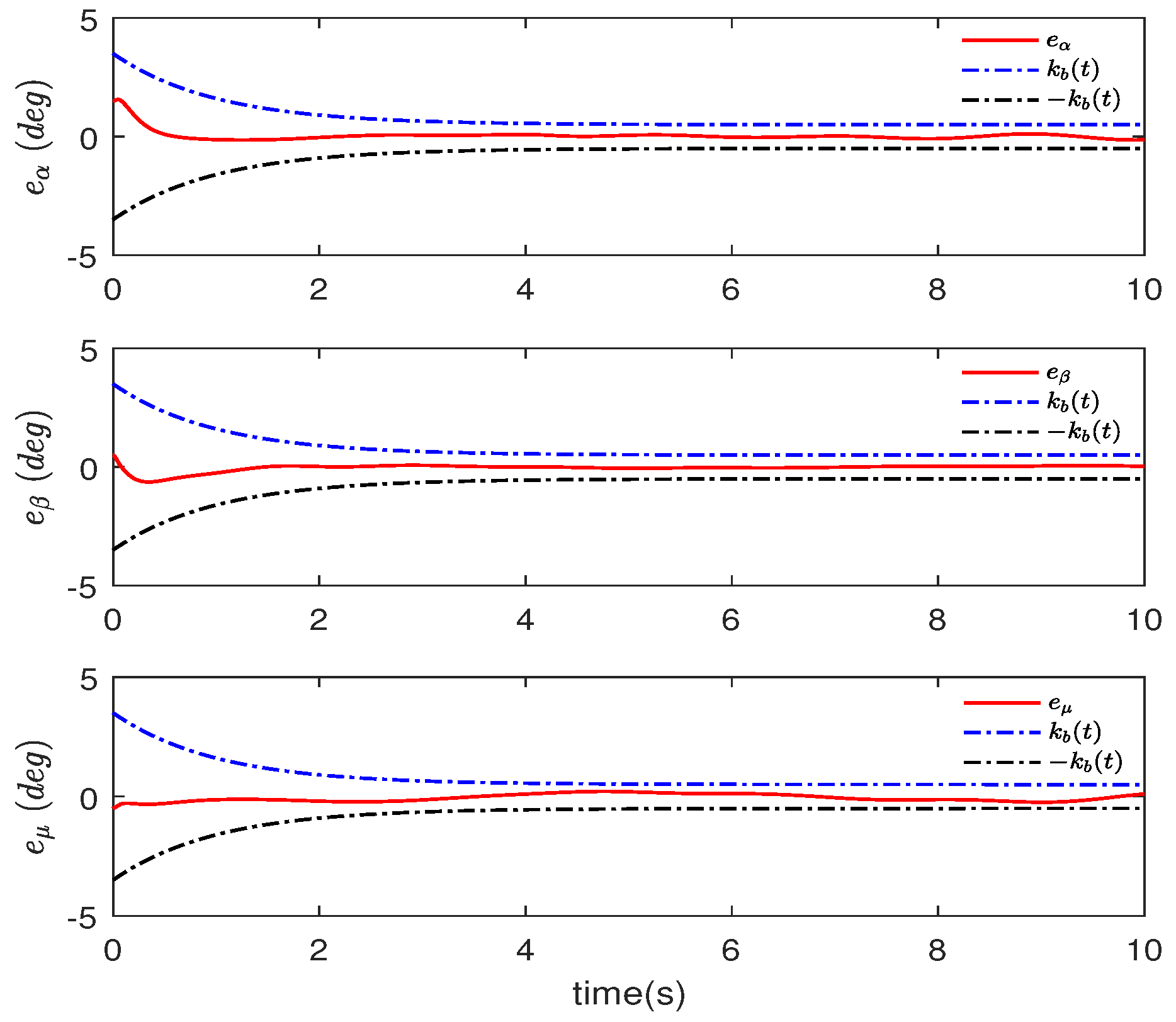
The tracking errors meet the output constraint requirements in the sense of probability.
(2)
All the closed-loop system signals are semi-globally uniform and ultimately bounded in the sense of probability. In particular, by selecting appropriate design parameters, the tracking error signals can converge to a small neighborhood ℵ in the sense of fourth-order moments, and ℵ is defined in the following form:
= { e 1 j ( t ) | E [ e 1 j 4 ] 8 Ξ ρ , t > T 0 , j = 1 , 2 , 3 }
where T 0 = max { 0 , 1 ρ ln ( ρ V ( 0 ) Ξ ) } .
Proof 
(1) When e 2 ι , selecting the Lyapunov candidate function as (52), according to (63), and combining with the proposed controller (64), the adaptive laws (65)–(67) and the compensation system (68), we have
L V L V 1 K 2 k b 4 2 π tan ( E 2 ) 1 4 η 13 4 G 1 4 C 1 4 e 2 4 C 2 2 L 2 2 η 21 C 2 e 2 2 cos 2 ( E 2 ) C 2 A ˜ 2 + C 2 L ϑ ˜ 2 ϑ ˜ 2 T ( S 2 L M ) ϑ ˜ 2 + Ψ e 2 4 Ψ ϕ 2 + ( e 2 T e 2 ) 2 + η 21 ϑ ˜ 2 T ϑ ˜ 2 + S 2 2 A ˜ 2 2 2 η 21 + t r { W ˜ 2 T Γ 2 1 W ^ ˙ 2 } + ε ¯ 2 e 2 T e 2 cos 2 ( E 2 ) e 2 ε ¯ 2 e 2 T e 2 cos 2 ( E 2 ) i = 1 3 e 2 i tanh ( e 2 i b 2 i ) + ε ¯ ˜ 2 ε ¯ ^ 2 + λ σ σ ¯ ˜ σ ¯ ^ + ϕ ϕ ˙ ζ 2 T C 2 ζ 2 + S 2 2 ϵ 2 2 2 η 21 + σ ¯ 2 2 + σ ¯ 2 η 22 χ T F 1 χ + η 23 2 χ 2 + B ¯ 2 2 η 23 + η 24 g 2 * 2 ζ 2 T ζ 2 + g 2 * Δ ¯ 2 2 η 24 L V 1 K 2 k b 4 2 π tan ( E 2 ) ϑ ˜ 2 T ( S 2 L M 3 η 21 2 I ) ϑ ˜ 2 1 4 η 13 4 G 1 4 C 1 4 e 2 4 C 2 e 2 2 cos 2 ( E 2 ) + S 2 2 A ˜ 2 2 2 η 21 + S 2 2 ϵ 2 2 2 η 21 + σ ¯ 2 2 + σ ¯ 2 η 22 λ 2 t r { W ˜ 2 T W ^ 2 } + ε ¯ 2 ϱ 2 e 2 T e 2 cos 2 ( E 2 ) + ε ¯ ˜ 2 ε ¯ ^ 2 + λ σ σ ¯ ˜ σ ¯ ^ + ϕ 2 Ψ ϕ 2 + ( e 2 T e 2 ) 2 + ϕ ϕ ˙ χ T F 1 χ + η 23 2 χ 2
+ B ¯ 2 2 η 23 + η 24 g 2 * 2 ζ 2 T ζ 2 + g 2 * Δ ¯ 2 2 η 24 L V 1 K 2 k b 4 2 π tan ( E 2 ) ϑ ˜ 2 T ( S 2 L M 3 η 21 2 I ) ϑ ˜ 2 1 4 η 13 4 G 1 4 C 1 4 e 2 4 + S 2 2 A ˜ 2 2 2 η 21 + S 2 2 ϵ 2 2 2 η 21 + σ ¯ 2 2 + σ ¯ 2 η 22 λ 2 t r { W ˜ 2 T W ^ 2 } + ε ¯ 2 2 ϱ 2 2 2 + ε ¯ ˜ 2 ε ¯ ^ 2 + λ σ σ ¯ ˜ σ ¯ ^ + ϕ 2 Ψ ϕ 2 + ( e 2 T e 2 ) 2 + ϕ ϕ ˙ χ T F 1 χ ζ 2 T C 2 ζ 2 + η 23 χ 2 2 + B ¯ 2 2 η 23 + η 24 g 2 * 2 ζ 2 T ζ 2 + g 2 * Δ ¯ 2 2 η 24
where ϱ 2 = ε ¯ 2 ς i = 1 3 b 2 i .
Based on (68) and Young inequality, one has
ϕ 2 Ψ ϕ 2 + ( e 2 T e 2 ) 2 + ϕ ϕ ˙ = κ ϕ ϕ 2
t r ( W ˜ 2 T W ^ 2 ) = W ˜ 2 2 2 + W ^ 2 2 2 W 2 * 2 2 W ˜ 2 2 2 W 2 * 2 2
ε ¯ ˜ 2 ε ¯ ^ 2 = 1 2 ( ε ¯ 2 2 ε ¯ ˜ 2 2 ε ¯ ^ 2 2 ) 1 2 ( ε ¯ 2 2 ε ¯ ˜ 2 2 )
σ ¯ ˜ σ ¯ ^ = 1 2 ( σ ¯ 2 σ ¯ ˜ 2 σ ¯ ^ 2 ) 1 2 ( σ ¯ 2 σ ¯ ˜ 2 )
Combining with (43), and substituting (71)–(74) into (70), thus one has
L V i = 1 2 K i k b 4 2 π tan ( E i ) i = 1 2 κ i ϑ ˜ i T ϑ ˜ i i = 1 2 λ ¯ i W ˜ i 2 𝚥 χ 2 ε ¯ ˜ 2 2 2 λ σ σ ¯ ˜ 2 2 2 κ ϕ ϕ 2 i = 1 2 𝚥 i ζ i T ζ i + i = 1 2 λ i W i * 2 2 + 3 η 13 3 4 4 + 1 2 η 15 d ¯ 1 2 + S 2 2 ε ¯ 2 2 2 + σ ¯ 2 2 + σ ¯ 2 η 2 + ε ¯ 2 2 2 + λ σ σ ¯ 2 2 2 + ε ¯ 2 2 ϱ 2 2 2 + B ¯ 2 2 η 22 + g 2 * Δ ¯ 2 2 η 24 ρ V + Ξ
where, ρ = min { 4 K i , 2 κ i , λ ¯ i λ m a x ( Γ i 1 ) , 2 𝚥 , ι 2 , λ σ τ ¯ , 2 κ ϕ } , κ 1 = λ m i n ( S 1 ) 1 2 η 11 η 14 2 η 15 2 > 0 , κ 2 = λ m i n ( S 2 L M ) 3 η 21 2 > 0 , λ ¯ 1 = λ 1 2 S 1 2 P 1 2 I 1 2 2 η 14 > 0 ,   λ ¯ 2 = λ 2 2 S 2 2 P 2 2 I 2 2 2 η 23 > 0 , 𝚥 = λ m i n ( F 1 ) 1 2 η 12 η 22 2 > 0 , 𝚥 1 = λ min ( C 1 ) η 16 g 1 * 2 > 0 , 𝚥 2 = λ min ( C 2 ) g 1 * 2 η 16 η 24 g 2 * 2 > 0 , Ξ = i = 1 2 λ i W i * 2 2 + 3 η 13 3 4 4 + d ¯ 1 2 2 η 15 + S 2 2 ε ¯ 2 2 2 + σ ¯ 2 2 + σ ¯ 2 η 2 + ε ¯ 2 2 2 + λ σ σ ¯ 2 2 2 + ε ¯ 2 2 ϱ 2 2 2 + B ¯ 2 2 η 22 + g 2 * Δ ¯ 2 2 η 24 .
(2) When e 2 < ι , based on (68), so that ϕ ˙ = 0 . Meanwhile, (71) can be rewritten as
ϕ 2 Ψ ϕ 2 + ( e 2 T e 2 ) 2 + ϕ ϕ ˙ = κ ϕ ϕ 2 + Λ
where Λ = κ ϕ ϕ 2 + ϕ 2 Ψ ϕ 2 + ( e 2 T e 2 ) 2 . Due to e 2 < ι , and ϕ is selected as a non-zero constant, it is easy to know that there exists a positive constant ν ¯ > 0 such that Λ ν ¯ .
Thus, (75) can be rewritten as
L V ρ V + Ξ ¯
where Ξ ¯ = Ξ + ν ¯ .
In order to analyze the probability boundedness of error signals, Ξ and Ξ ¯ are uniformly expressed by Ξ * . Furthermore, combining with (75) and (77), one has
d E [ V ] d t ρ E [ V ] + Ξ *
Then, it can be obtained that
E [ V ] ( V ( 0 ) Ξ * ρ ) e ρ t + Ξ * ρ e ρ t V ( 0 ) + Ξ * ρ
Therefore, this means that the mean value of V is convergent and satisfies the output constraint requirement in the sense of probability.
Futhermore, owing to
e 1 j 4 ( e 1 T e 1 ) 2 2 k b 4 π tan ( π ( e 1 T e 1 ) 2 2 k b 4 ) 4 V
So then, we have
E [ e 1 j 4 ] 4 E [ V ] 8 Ξ * ρ , t > T 0
where T 0 = max { 0 , 1 ρ ln ( ρ V ( 0 ) Ξ * ) } .
Therefore, it is obvious that the tracking error signals converge to a small neighborhood of zero in the sense of the fourth moment. □

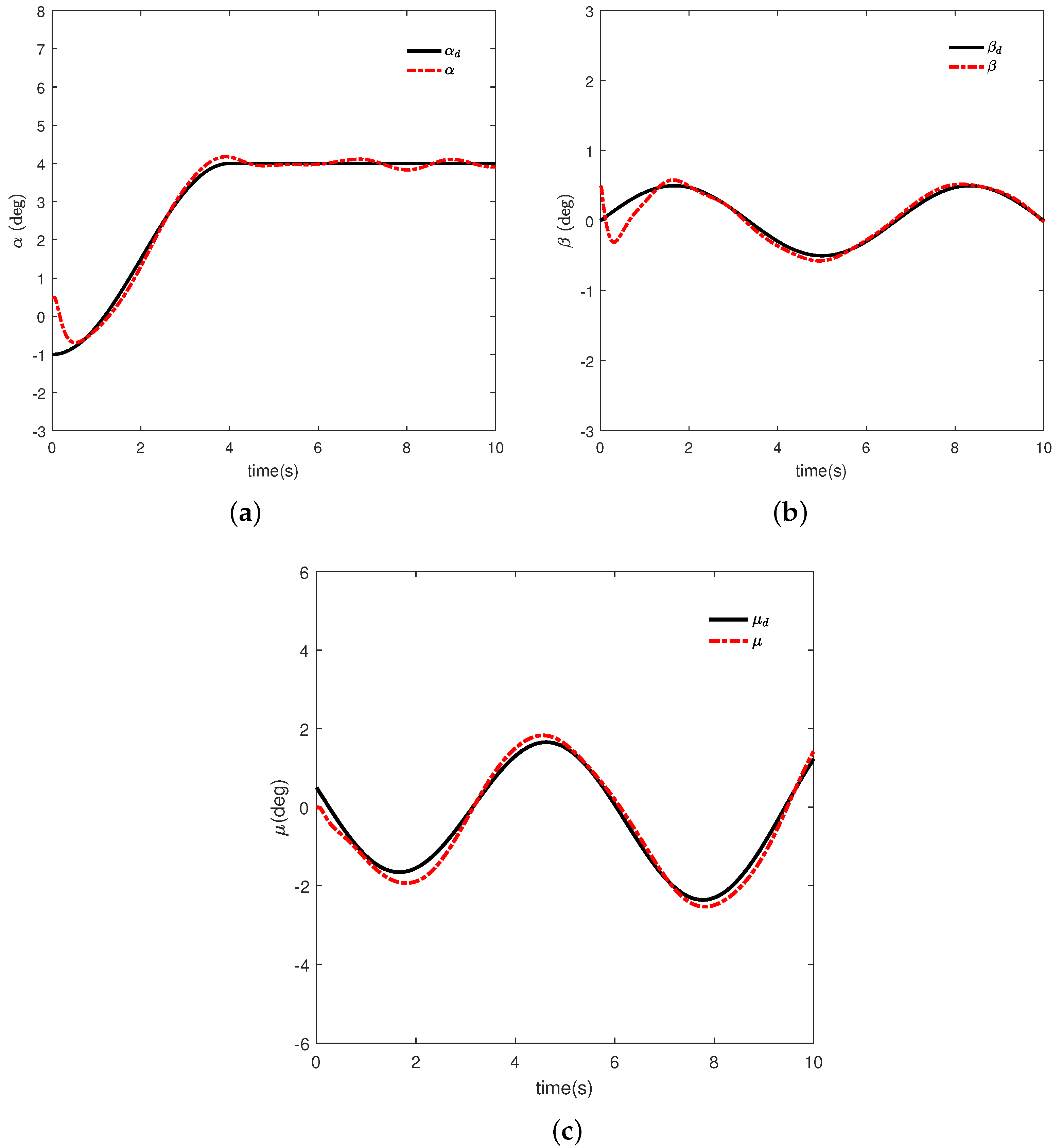
5. Simulation Results

In this section, considering the influence of multi-source disturbances, input–output constraints and system uncertainties, numerical simulation analysis is carried out for the attitude nonlinear system of the NSV to illustrate the feasibility and effectiveness of the adaptive robust stochastic control scheme based on the NDO, auxiliary system and TBLF. The physical structure parameters of the NSV are shown in Table 1.
In the simulation process, it is assumed that there exists system uncertainty of ±(20%) for the aerodynamic force and aerodynamic moment coefficients of the NSV attitude system model. Consider the control surface deflection angle δ e , δ a and δ r as the actual control inputs, which are affected by stochastic noises σ i ξ 1 i ( i = 1 , 2 , 3 ) , denoting stochastic input moment disturbance d ¯ ( t ) = G δ Σ ξ 1 , where Σ = d i a g { σ 1 , σ 2 , σ 3 } , and ξ 1 = [ ξ 11 , ξ 12 , ξ 13 ] T with ξ 1 i being the standard Gaussian white noise. As described in [7], the moment disturbance d ¯ ( t ) acting on the fast-loop subsystem in the form of torque.
In addition, the external time-varying disturbance d 1 ( t ) = 0.02 · [ sin ( 2 t ) e 0.1 t , sin ( t ) e 0.1 t , sin ( 2 t ) e 0.1 t ] T is added to the slow-loop subsystem, and another kind of external disturbance d 2 ( t ) = [ d 21 ( t ) , d 22 ( t ) , d 23 ( t ) ] T with partial known information is added to the fast-loop subsystem, where d 2 j ( t ) is generated by the following exosystem:
ϖ ˙ j = M j ϖ j + N j ξ j , d 2 j ( t ) = L j ϖ j
Meanwhile, setting σ 1 = σ 2 = σ 3 = 0.05 , the system matrices of (82) are chosen as: M 1 = M 2 = M 3 = 0 3 3 0 , N 1 = N 2 = N 3 = 1 0 0 1 , L 1 = 0 2 , L 2 = 3 0 , L 3 = 1 1 .
The initial values of relevant parameters of the NSV are shown in Table 2, and the corresponding sampling period is chosen as 0.002 s. According to the physical characteristics of the NSV, the saturation value of control input moment is set to u ¯ M = [2000, 20,000, 20,000] T kN·m. The constraint function of the output tracking error is chosen as k b ( t ) = 3 e t + 0.5 , and the desired reference attitude angle signals are selected as
Ω r = α r = [ 2.5 sin ( 0.25 π t 0.5 π ) + 1.5 ] d e g , 0 t 4 4 d e g , t > 4 β r = 0.5 sin ( 0.3 π t ) d e g , μ r = [ 2 sin ( t ) + 0.5 cos ( 0.5 t ) ) ] d e g
In order to compensate for the influence of input saturation, an auxiliary system is designed as (13), and the matrix parameters are C 1 = d i a g { 20 , 20 , 20 } and C 2 = d i a g { 50 , 50 , 50 } . Meanwhile, the NDOs are designed as (21) and (50) to estimate the external disturbances d 1 ( t ) and d 2 ( t ) . The gain matrices of the NDO are chosen as follows:
S 1 = 10 0 0 0 10 0 0 0 10 , S 2 = 1.5 1.5 0 0 0 0 0 0 1.5 1 0 0 0 0 0 0 2 4 T ,
In addition, the relevant parameters of controller and adaptive updating laws are selected as shown in Table 3.
For the stochastic nonlinear system (11) of the NSV attitude system, it is necessary to use six MTPNs to approximate the uncertainties, and the structural form of MTPN is in accordance with (4). For the intermediate layer of MTPN, the sum of the highest powers of the product terms can be selected as 3; that is, the number of nodes is l 1 j = l 2 j = 19 , j = 1 , 2 , 3 .
By selecting appropriate control parameters, the NSV attitude motion simulation results are shown in Figure 3, Figure 4, Figure 5, Figure 6 and Figure 7. Figure 3 and Figure 4 describe the estimation performance response and disturbances estimation errors of the designed NDO. It can be seen that the designed NDO can estimate external disturbances, and the estimation errors converge to a sufficiently small neighborhood of zero. In Figure 5, we can see the tracking effect of the NSV attitude angle, and the system output signals can quickly track the desired reference attitude angle signals. The attitude tracking performance and output constraint conditions of the NSV are shown in Figure 6. It can be seen that the tracking error signals can quickly converge to a small neighborhood and meet the preset output constraint requirements. Figure 7 shows the saturated control input. Therefore, through the analysis of the above simulation results, it is obvious that the proposed adaptive robust stochastic control scheme based on the NDO, MTPN and TBLF in this paper can effectively ensure that NSV has satisfactory flight control performance.

6. Conclusions

In order to obtain high precision flight control performance, it is also necessary to fully consider the influence of different types of external disturbances to improve the robustness of the NSV flight control system. Meanwhile, the input and output constraint requirements must be considered in the safe flight control of NSVs. In this paper, the attitude tracking control problem of the NSV with multi-source disturbances, input and output constraints and system uncertainties is considered, and an adaptive robust stochastic control scheme is proposed based on the NDO, MTPN and TBLF. By means of the stochastic Lyapunov stability theory, the probability boundedness of the closed-loop system signals are proved. In future research, it will be necessary to consider multiple time-varying switching disturbances (such as wind disturbances, hypersonic magnetic fluid interference, etc.). By integrating the stochastic Markov jump system theory and the processing technology for output constraint, the advanced flight control scheme needs to be developed to ensure the reliable flight of the NSV.

Author Contributions

Conceptualization, X.Y.; Methodology, X.Y. and Q.Y.; Software, G.S., L.Y. and S.T.; Writing—original draft, X.Y. and G.S.; Writing—review & editing, Q.Y. and Y.Y. All authors have read and agreed to the published version of the manuscript.

Funding

This research was funded by National Natural Science Foundation of China under Grant 61825302 and Grant 61903118, the Natural Science Foundation of Anhui Province under Grant 1908085QF290, the Natural Science Foundation of Shandong Province under Grant ZR2017LF013, the project of Ministry of Industry and Information Technology of China under Grant TC210804V-1, and the Talent Foundation of Hefei University under Grant 20RC27.

Data Availability Statement

Not applicable.

Conflicts of Interest

The authors declare no conflict of interest.

References

  1. Cui, E. Research statutes, development trends and key technical problems of near space vehicles. Adv. Mech. 2009, 39, 658–673. [Google Scholar]
  2. Bu, X.; Wu, X.; Ma, Z.; Zhang, R. Novel Adaptive Neural Control of Flexible Air-breathing Hypersonic Vehicles Based on Sliding Mode Differentiator. Chin. J. Aeronaut. 2015, 28, 1209–1216. [Google Scholar] [CrossRef]
  3. Xu, H.; Mirmirani, M.; Ioannou, P. Adaptive sliding mode control design for a hypersonic flight vehicle. J. Guid. Control Dyn. 2004, 27, 829–838. [Google Scholar] [CrossRef]
  4. Wang, Y.; Jiang, C.; Wu, Q. Attitude tracking control for variable structure near space vehicles based on switched nonlinear systems. Chin. J. Aeronaut. 2013, 26, 186–193. [Google Scholar] [CrossRef]
  5. Wu, H.; Liu, Z.; Guo, L. Robust -gain fuzzy disturbance observer-based control design with adaptive bounding for a hypersonic vehicle. IEEE Trans. Fuzzy Syst. 2013, 22, 1401–1412. [Google Scholar] [CrossRef]
  6. Xu, B. Robust adaptive neural control of flexible hypersonic flight vehicle with dead-zone input nonlinearity. Nonlinear Dyn. 2015, 80, 1509–1520. [Google Scholar] [CrossRef]
  7. Yan, X.; Chen, M.; Shao, S.; Wu, Q. Polynomial networks based adaptive attitude tracking control for NSVs with input constraints and stochastic noises. Chin. J. Aeronaut. 2021, 34, 124–134. [Google Scholar] [CrossRef]
  8. Shao, S.; Chen, M. Robust discrete-time fractional-order control for an unmanned aerial vehicle based on disturbance observer. Int. J. Robust Nonlinear Control 2022, 32, 4665–4682. [Google Scholar] [CrossRef]
  9. Shao, S.; Chen, M.; Hou, J.; Zhao, Q. Event-triggered-based discrete-time neural control for a quadrotor UAV using disturbance observer. IEEE/ASME Trans. Mechatron. 2021, 26, 689–699. [Google Scholar] [CrossRef]
  10. Ren, Y.; Zhao, Z.; Ahn, C.; Li, H. Adaptive fuzzy control for an uncertain axially moving slung-load cable system of a hovering helicopter with actuator fault. IEEE Trans. Fuzzy Syst. 2022, in press. [Google Scholar] [CrossRef]
  11. Su, J.; Chen, W.; Yang, J. On relationship between time-domain and frequency-domain disturbance observers and its applications. J. Dyn. Syst. Meas. Control 2016, 138, 091013. [Google Scholar] [CrossRef] [Green Version]
  12. Chen, W. Nonlinear disturbance observer-enhanced dynamic inversion control of missiles. J. Guid. Control Dyn. 2003, 26, 161–166. [Google Scholar] [CrossRef]
  13. Li, X.; Xian, B.; Chen, D.; Yu, Y.; Zhang, Y. Output feedback control of hypersonic vehicles based on neural network and high gain observer. Sci. China Inf. Sci. 2011, 54, 429–447. [Google Scholar] [CrossRef]
  14. Yang, J.; Li, S.; Sun, C.; Guo, L. Nonlinear-disturbance-observer-based robust flight control for air-breathing hypersonic vehicles. IEEE Trans. Aerosp. Electron. Syst. 2013, 49, 1263–1275. [Google Scholar] [CrossRef]
  15. Chen, M.; Ren, B.; Wu, Q.; Jiang, C. Anti-disturbance control of hypersonic flight vehicles with input saturation using disturbance observer. Sci. China Inf. Sci. 2015, 58, 1–12. [Google Scholar] [CrossRef]
  16. Xu, B.; Wang, D.; Zhang, Y.; Shi, Z. DOB-based neural control of flexible hypersonic flight vehicle considering wind effects. IEEE Trans. Ind. Electron. 2017, 64, 8676–8685. [Google Scholar] [CrossRef]
  17. Wu, H.; Feng, S.; Liu, Z.; Guo, L. Disturbance observer-based robust mixed H2/H fuzzy tracking control for hypersonic vehicles. Fuzzy Sets Syst. 2017, 306, 118–136. [Google Scholar] [CrossRef]
  18. Sinha, A.; Miller, D. Optimal sliding-mode control of a flixible spacecraft under stochastic disturbances. J. Guid. Control. Dyn. 1995, 18, 486–492. [Google Scholar] [CrossRef]
  19. Liu, M.; Zhang, L.; Shi, P. Robust control of stochastic systems against bounded disturbances with application to flight control. IEEE Trans. Ind. Electron. 2013, 61, 1504–1515. [Google Scholar] [CrossRef]
  20. Samiei, E.; Izadi, M.; Viswanathan, S.; Sanyal, A.; Butcheret, E. Robust stabilization of rigid body attitude motion in the presence of a stochastic input torque. In Proceedings of the 2015 IEEE International Conference on Robotics and Automation, Seattle, WA, USA, 26–30 May 2015; pp. 428–433. [Google Scholar]
  21. Chen, B.; Wang, C.; Lee, M. Stochastic robust team tracking control of MIMO-UAV networked system under wiener and poisson random fluctrations. IEEE Trans. Cybern. 2020, 51, 5786–5799. [Google Scholar] [CrossRef]
  22. Lv, M.; Li, Y.; Pan, W.; Baldi, S. Finite-time fuzzy adaptive constrained tracking control for hypersonic flight vehicles with singularity-free switching. IEEE/ASME Trans. Mechatronics 2022, 27, 1594–1605. [Google Scholar] [CrossRef]
  23. Zhao, Z.; Ren, Y.; Mu, C.; Zou, T.; Hong, K. Adaptive neural-network-based fault-tolerant for a flexible string with composite disturbance observer and input constraints. IEEE Trans. Cybern. 2021, in press. [Google Scholar] [CrossRef] [PubMed]
  24. Yan, X.; Chen, M.; Feng, G.; Wu, Q.; Shao, S. Fuzzy robust constrained control for nonlinear systems with input saturation and external disturbances. IEEE Trans. Fuzzy Syst. 2021, 29, 345–356. [Google Scholar] [CrossRef]
  25. Shao, S.; Chen, M. Adaptive neural discrete-time fractional-order control for an UAV system with prescribed performance using disturbance observer. IEEE Trans. Syst. Man Cybern. Syst. 2021, 51, 742–754. [Google Scholar] [CrossRef]
  26. Ren, Y.; Zhao, Z.; Zhang, C.; Yang, Q.; Hong, K. Adaptive neural-network boundary control for a flexible manipulator with input constraints and model uncertainties. IEEE Trans. Cybern. 2021, 51, 4796–4807. [Google Scholar] [CrossRef] [PubMed]
  27. Zhao, Z.; Zhang, J.; Liu, Z.; Mu, C.; Hong, K. Adaptive neural network control of an uncertain 2-DOF helicopter with unknown backlash-like hysteresis and output constraints. IEEE Trans. Neural Netw. Learn. Syst. 2022, in press. [Google Scholar] [CrossRef]
  28. Khas’Miniskii, R. Stochastic Stability of Differential Equations; Springer: Berlin/Heidelberg, Germany, 1980. [Google Scholar]
  29. Yan, H.; Kang, A. Asymptotic tracking and dynamic regulation of SISO nonlinear system based on discrete multi-dimensional Taylor network. IET Control. Theory Appl. 2017, 11, 1619–1626. [Google Scholar] [CrossRef]
  30. Han, Y.; Zhu, S.; Yang, S. Adaptive multi-dimensional Taylor network tracking control for a class of stochastic nonlinear systems with unknown input dead-zone. IEEE Access 2018, 6, 34543–34554. [Google Scholar] [CrossRef]
  31. Wang, H.; Liu, X.; Liu, K.; Karimi, H. Approximation-based adaptive fuzzy tracking control for a class of nonstrict-feedback stochastic nonlinear time-delay systems. IEEE Trans. Fuzzy Syst. 2015, 23, 1746–1760. [Google Scholar] [CrossRef]
  32. Du, Y.; Wu, Q.; Jiang, C.; Xue, Y. Adaptive recurrent-functional-link-network control for hypersonic vehicles with atmospheric disturbances. Sci. China Inf. Sci. 2011, 54, 482–497. [Google Scholar] [CrossRef]
Figure 1. The external disturbances generated by an exosystem: (a) harmonic disturbance with known frequencies; (b) external disturbance with random excitation.
Actuators 11 00273 g001
Figure 2. Robust adaptive control structure diagram.
Actuators 11 00273 g002
Figure 3. Slow-loop disturbance estimation response curve of the NDO: (a) d 1 and d ^ 1 (rad/s); (b) the estimation error d ˜ 1 (rad/s).
Actuators 11 00273 g003
Figure 4. Fast-loop disturbance estimation response curve of the NDO: (a) d 2 and d ^ 2 (rad/s 2 ); (b) the estimation error d ˜ 2 (rad/s 2 ).
Actuators 11 00273 g004
Figure 5. Tracking response curves of attitude angles: (a) pitch angle α ; (b) yaw angle β ; (c) roll angle μ .
Actuators 11 00273 g005
Figure 6. Constrained tracking error response curves of attitude angles.
Actuators 11 00273 g006
Figure 7. Control input moment response curve.
Actuators 11 00273 g007
Table 1. The physical structure parameters of NSV (partly).
MeaningValueUnit
vehicle length60.69m/s
vehicle mass136,820kg
reference area334.73m 2
mean aerodynamic chord24.384m
wing string length18.288m
sweep angle75.97deg
rudder chord length6.9494m
Table 2. Simulation initial parameters.
VariableIntial ValueUnit
velocity V 0 = 3000 m/s
height H 0 = 22,000m
pitch angle α 0 = 0.5 deg
yaw angle β 0 = 0.5 deg
roll angle μ 0 = 0 deg
angular rate p 0 = q 0 = r 0 = 0 deg/s
Table 3. Relevant simulation parameters of the controller and adaptive laws.
Parameter VariableValueParameter VariableValue
k ¯ 1 2 τ ¯ 1
K 1 diag { 1.5 , 1.5 , 1.5 } ζ 1
K 2 diag { 2 , 2 , 2 } ι 0.01
ι 1 = ι 2 0.1 κ ϕ 2
η 11 = η 12 = η 13 1 F diag { 0.1 , 0.1 , 0.1 }
η 21 = η 22 0.1 Γ 1 = Γ 2 I 19
λ 1 = λ 2 = λ σ 0.1 b2
Publisher’s Note: MDPI stays neutral with regard to jurisdictional claims in published maps and institutional affiliations.

