2.1. Computational Model
The typical dimensions of shield tunnels in China were selected for this study.
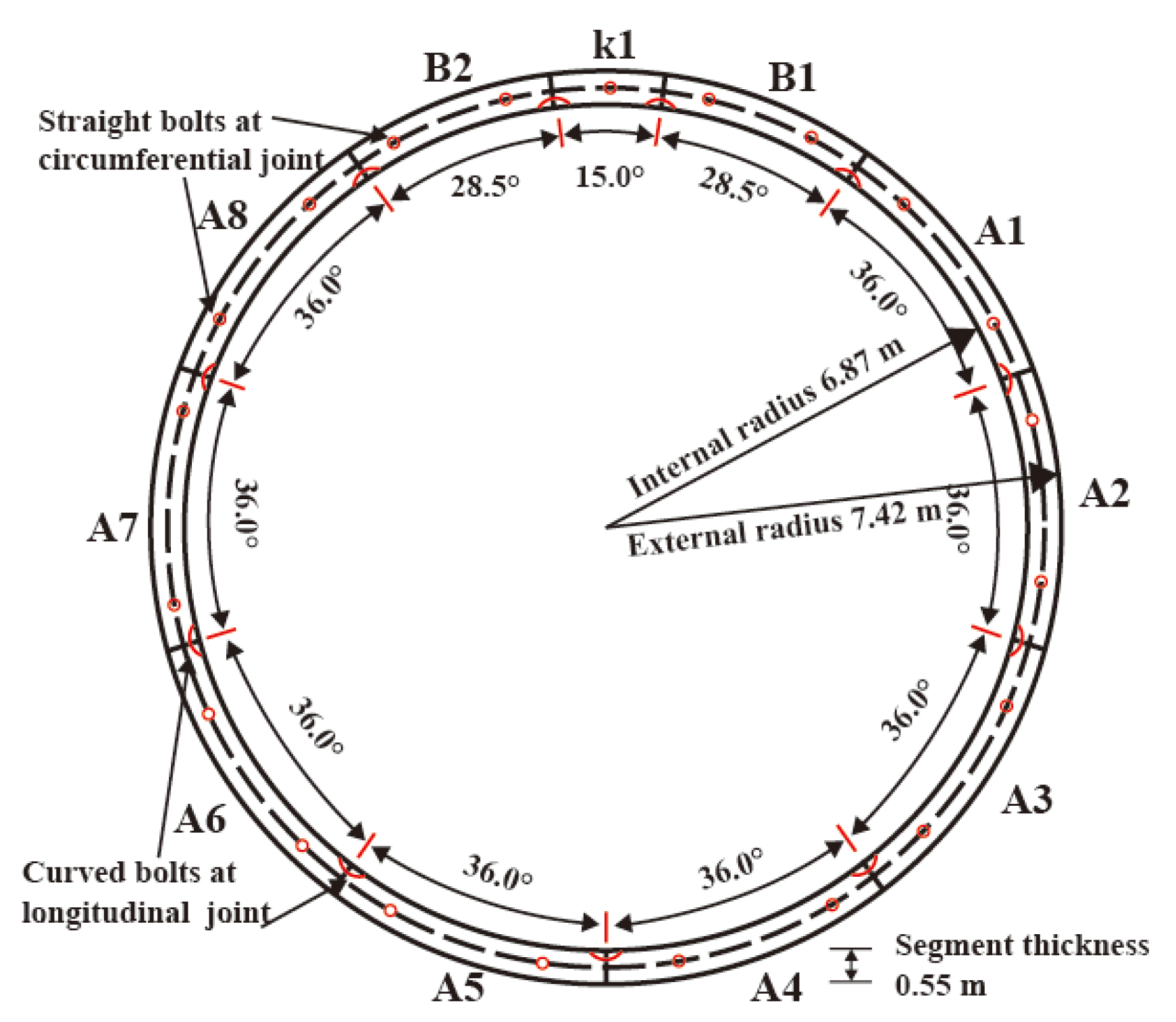
Figure 1 shows a cross-sectional schematic of a shield tunnel segment structure. The inner and outer radii of the tunnel are 6.87 m and 7.42 m, respectively; the thickness and width of each ring pipe piece are 0.55 m and 2.0 m, respectively; and the segments are connected by staggered seams. Each segment lining ring consists of eight standard blocks A1–A8 (36°), two neighboring blocks B1–B2 (28.5°), and one capping block k1 (15°). The longitudinal and circumferential joints of the segment lining ring were assembled using 30 mm diameter 8.8 grade high-strength bending bolts and straight bolts, respectively. A preload force of 280 kN was applied to the friction-type bolts; the preload force values were selected from the Code for Structural Steel Design [
15] and applied through the load module in the 2020 ABAQUS software.
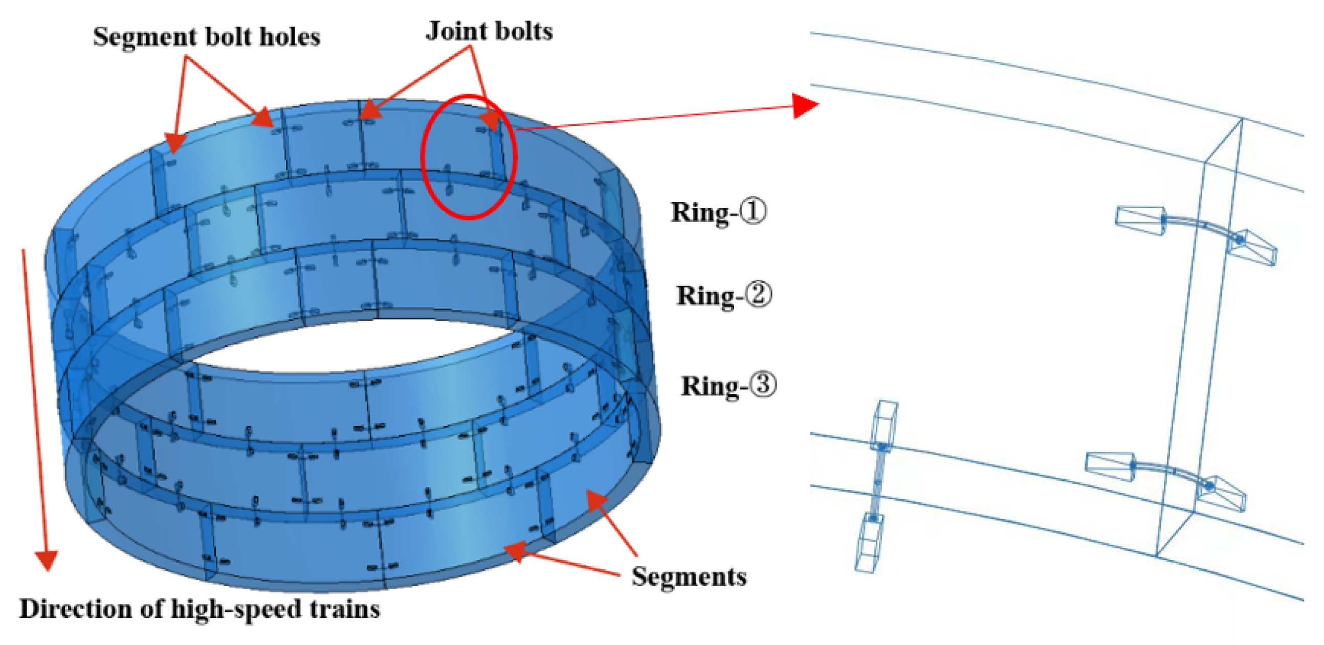
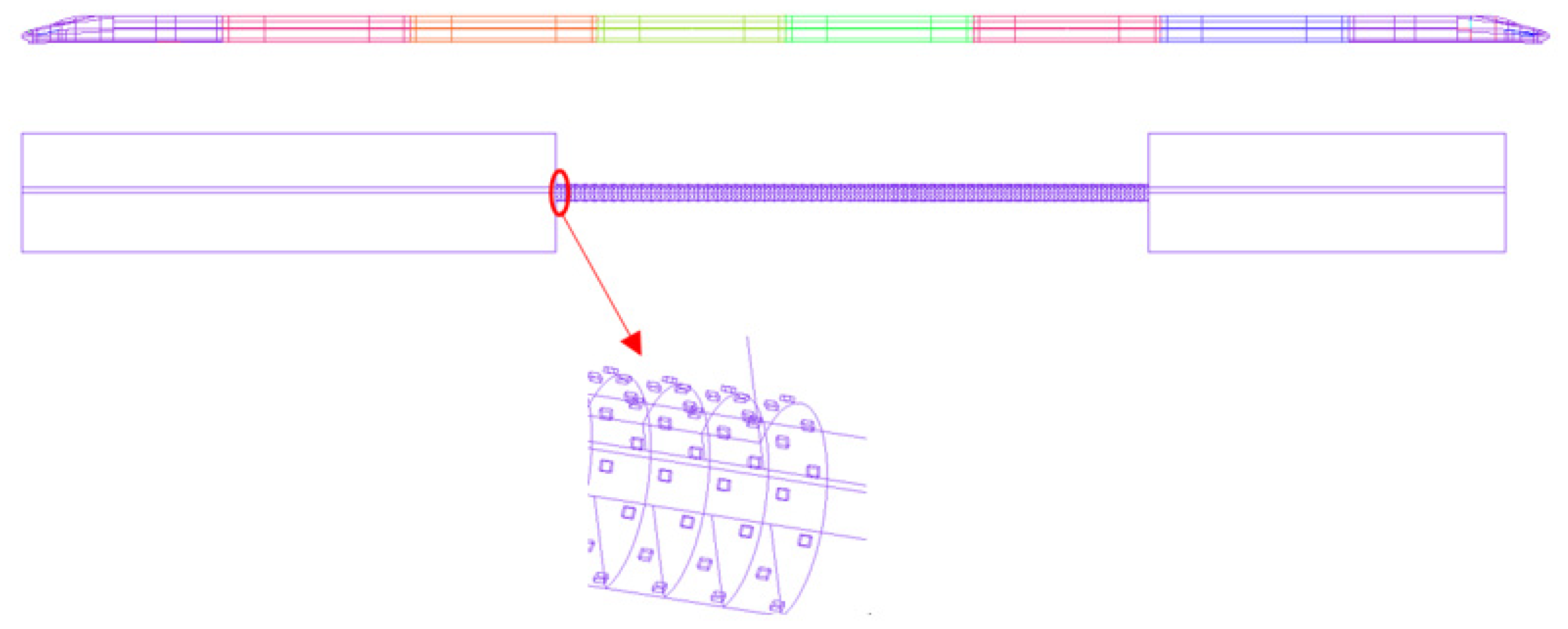
Figure 2 shows a 3D finite element model of the shield tunnel, including the segment lining rings and joint bolts, three-segment rings with bending bolt connections for the annular pieces, and straight bolt connections for the longitudinal pieces (the direction of train travel). The holes in the high-strength bolts were considered in order to better represent the actual conditions. In the numerical calculations, surface-to-surface contact was used between the segments, between the bolts and the segment, and between the lining rings of the adjacent segments before and after. Hard contact was used in the normal direction and Mohr–Coulomb friction contact was used in the tangential direction; the friction coefficient was taken as 0.6 [
16]. Surface-to-surface contact was set up between the lined segment and surrounding rock; the normal direction used a penalty stiffness [
17] and the tangential direction used Mohr–Coulomb friction contact with a friction coefficient of 0.8. The segment and elevated arch were considered to be in coordinated deformation, and a tie contact was used.
As the model underwent dynamic analysis, the infinite range of the surrounding rock was a key problem in analyzing dynamic interaction. If the selected model range is too large, a significant amount of time is wasted in numerical calculation and storage, and the model may be impossible to complete. At this time, part of the surrounding rock was used for finite domain analysis; thus, it was necessary to set viscoelastic artificial boundary conditions. Liu et al. [
18] proposed the concept of artificial boundary conditions and derived an equation for equivalent and consistent viscoelastic boundary conditions that was then verified. The main equations for the equivalent shear model and equivalent elastic model of boundary cells are shown in (1):
where
, and
are the equivalent elastic model, shear model, and Poisson’s ratio of the equivalent viscoelastic boundary condition unit, respectively,
,
,
is the thickness of the equivalent unit,
and
are the tangential and normal spring stiffnesses, respectively,
and
are the tangential and normal viscoelastic artificial boundary parameters, respectively, with
generally taking values in the range of 0.35–0.65 and
generally taking values in the range of 0.8–1.2,
is the medium shear modulus, and
is the distance from the wave source to the artificial boundary point.
Considering the vibration effect of the train, corresponding damping options should be set when analyzing the dynamic response of the soil and lining structure. The numerical simulation in this study uses Rayleigh damping; two key parameters, the damping ratio and minimum center frequency, must be determined, as shown in Equation (2).
where
is the critical damping ratio,
is the minimum central frequency, and
and
are constants associated with mass and stiffness, respectively. The formula is
, where
, and
are the damping matrix, mass matrix, and stiffness matrix, respectively.
According to the monograph by Chen and Xu [
19], the critical damping ratio of geotechnical materials generally ranges from 2–5% and the critical damping ratio of structural systems ranges from 2–10%. In this study, the critical damping ratio of the surrounding rock in the numerical calculation was 3% and the damping ratio of the tunnel structure was 5%.
A three-dimensional stratigraphic–structural model was established using ABAQUS software, with a distance of 30 m from the tunnel vault to the ground surface. To reduce the boundary effect, the distance from the constrained boundary to the tunnel center is generally 3–5 times the tunnel span; in this study, the distance from the center of the tunnel to the constrained boundary was four times the tunnel span and the distance from the bottom of the tunnel to the center of the tunnel was three times the tunnel span. The final model size was 120 m × 90 m × 6 m.
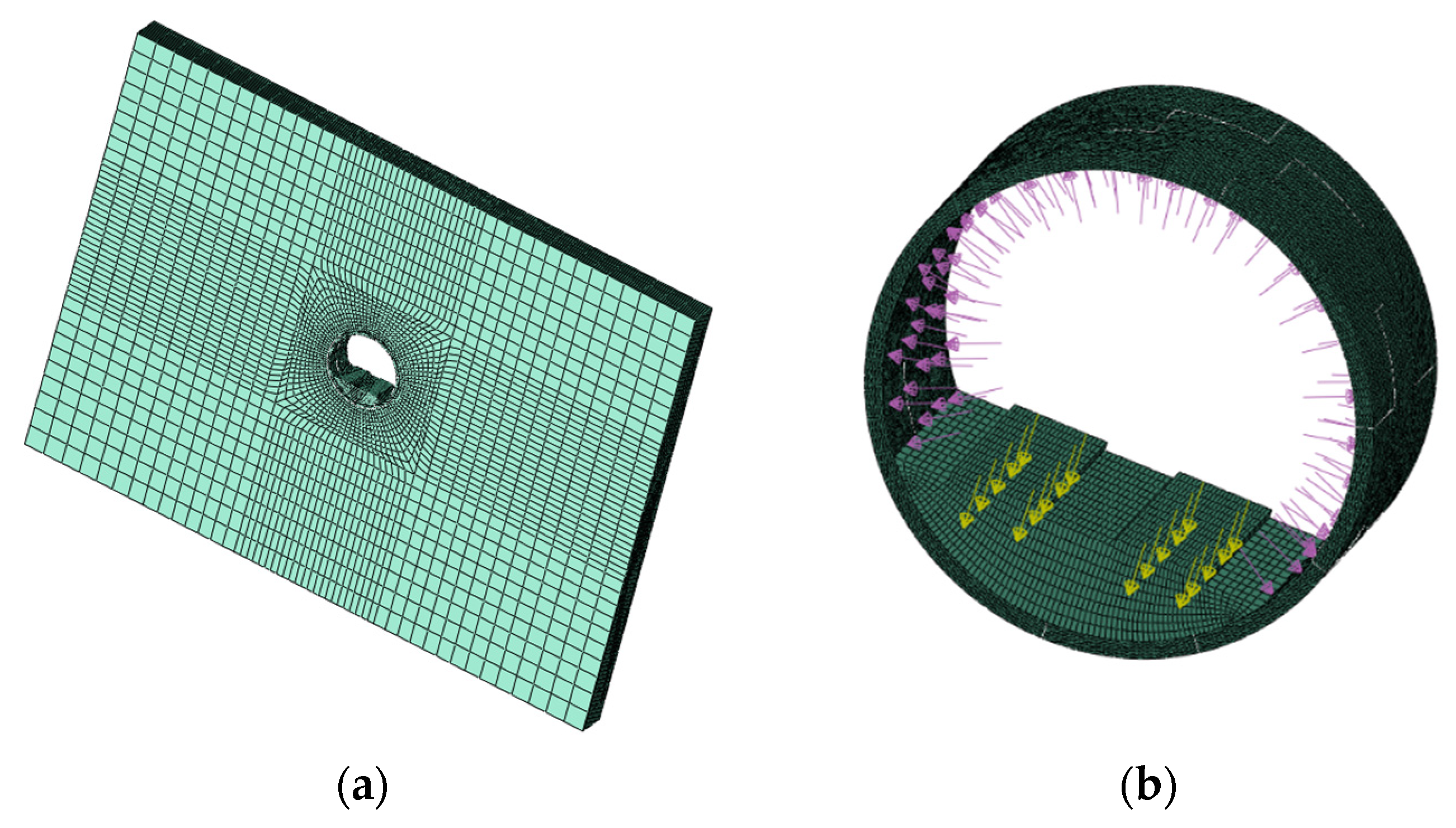
Figure 3 shows the finite element model of the surrounding rock and lining structure.
Figure 3a shows the surrounding rock grid and
Figure 3b shows a diagram of the pneumatic and vibration loads applied on the lining wall and rail slab.
To improve calculation efficiency and ensure calculation accuracy, parts of the analysis, such as the segment structure and high-strength bolts, were refined and modeled. The rest of the segment structure was homogenized according to the principle of equivalent flexural stiffness [
20], calculated using Equation (3).
where
E is the equivalent modulus of elasticity of the segment structure, I is the moment of inertia of the homogeneous model cross-section to the neutral axis, taken as 1.75 × 10
−5 m
4 [
21],
are the modulus of elasticity of steel reinforcement and concrete, respectively,
are the moments of inertia on the neutral axis of steel reinforcement and concrete, respectively, where
,
is the diameter of steel reinforcement (32 mm),
is the unit length (1000 mm), and
is the segment structure width (550 mm).
Because the two parameters of the Mohr–Coulomb model are easily obtained and widely used in underground engineering, the surrounding rock in the tunnel was calculated using the Mohr–Coulomb model. According to Pan [
22], when a shield tunnel is excavated the ground stress is released, and can be considered at this time by the parametric softening method; the surrounding rock to be excavated is discounted by 30% of the elastic modulus, and the initial stress state of the shield tunnel lining structure during operation can be calculated. At this time, following to the parameter values and reduction coefficients in the literature [
22], the surrounding rock parameters used in this paper are shown in
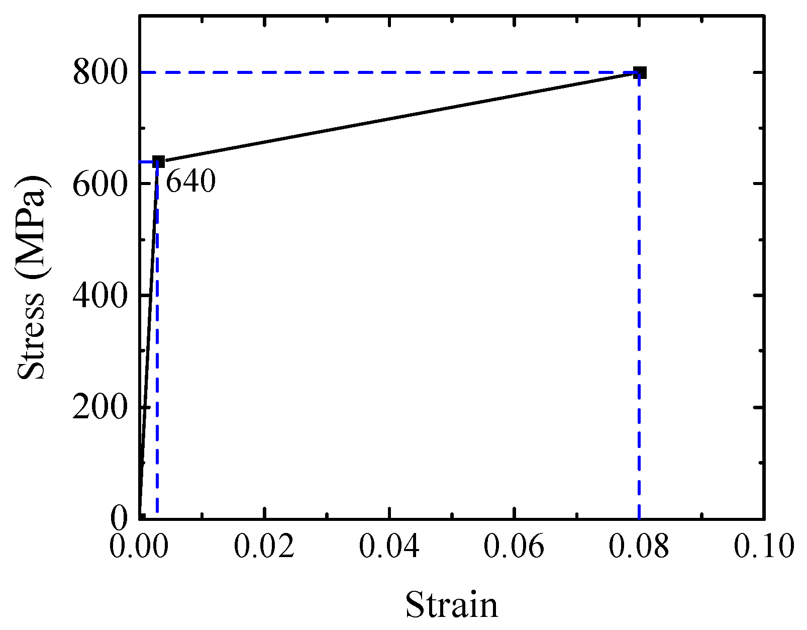
Table 1. The lining concrete of the segment was subject to the elastic–plastic damage CDP model established from the literature [
23,
24]. The joint bolts were modeled as linearly elastic, the concrete grade of the shield tunnel segment was C50, and the inverted arch and rail slab were made of C30 concrete. The relevant parameters for the segment lining, inverted arch, rail slab, and high-strength bolts in
Table 1 were obtained according to code [
25]. The physical parameters required by the specific model are shown in
Table 1.
2.2. Determination of Most Unfavorable Pneumatic Load
The aerodynamic pressure wave generated when two trains meet in a tunnel is much larger than that generated when a single train runs through the tunnel. Consider two trains meeting in the middle of a tunnel. When the head of train A enters the tunnel, a compression wave propagates to the tunnel exit to form an expansion wave. When the rear of train B enters the tunnel, the two are superimposed, resulting in stronger expansion wave action on train B. The compression waves generated by the heads of trains A and B pass through the entire tunnel at the same time. If the tunnel is too long, the compression waves are attenuated in the tunnel; if the tunnel is too short, the effect of the compression waves is inadequate, and the tunnel length is unfavorable.
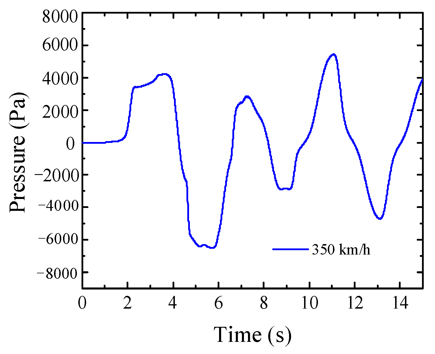
Based on this principle, Equation (4) can be obtained as follows. With a train speed of 350 km/h, the most unfavorable tunnel length was calculated to be approximately 700 m; the result from Equation (4) was consistent with the calculation result when using the formula in the railway industry standard of the People’s Republic of China (TB/T 3503.3-2018) [
26]. The time–pressure curve of the pneumatic pressure wave at the central measurement point of the shield tunnel at a height of 1.5 m from the track surface at this speed was derived using a slip grid and Fluent software, as shown in
Figure 4. The details of the boundary condition settings and model validation for calculation of the aerodynamic loads are provided in the literature [
27,
28,
29,
30].
where
is the most unfavorable tunnel length when trains meet in the tunnel at equal speeds,
is the length of the high-speed trains (203 m),
is the speed of the trains, and
is the speed of sound (335 m/s).
2.3. Determination of Vibration Load and Method Validation
Factors affecting the train vibration load include the train speed, train and rail type, and irregularity, which make it more difficult to determine the train load. High-speed railroad routes are mostly seamless lines with integral roadbeds. The irregularity of the track and the waveform wear effect of the rail surface are the most direct causes of train vibration loads. Most current irregularity management values use British standards [
31], as shown in
Table 2.
At this stage, there are three methods to determine the vibration load of the train, (1) field measurements [
32] or inversion of the vibration load of the train based on spectrum analysis [
33], although the results obtained using this method are highly discrete; (2) the coupled train–track modeling method, which is too complex in terms of the model and parameters, and insufficiently clear in modeling the wheel–rail contact relationship [
34]; or (3) an empirical formula able to accurately represent the vibration load using a simple expression. Liang et al. [
31] modified and improved the train load expression proposed by Pan and GN [
35] by fully considering the mechanism of vibration load generation (including the train factor, under-rail foundation factor, etc.). The excitation force function they used can better simulate the train vibration load, as shown in Equation (5):
where
is the static load of wheel action,
,
, and
are the corresponding peak power loads,
is the superposition coefficient of adjacent wheel–rail force,
is the rail dispersion coefficient,
is generally taken as 1.2~1.7, and here as 1.6,
is generally taken as 0.6~0.9, and here as 0.8,
is the vibration circle frequency in the unevenness control condition,
is the time,
represents the peak power load in the three control conditions,
is the typical vector height in mm,
is the typical wavelength of the geometrically uneven curve, and
is the train speed.
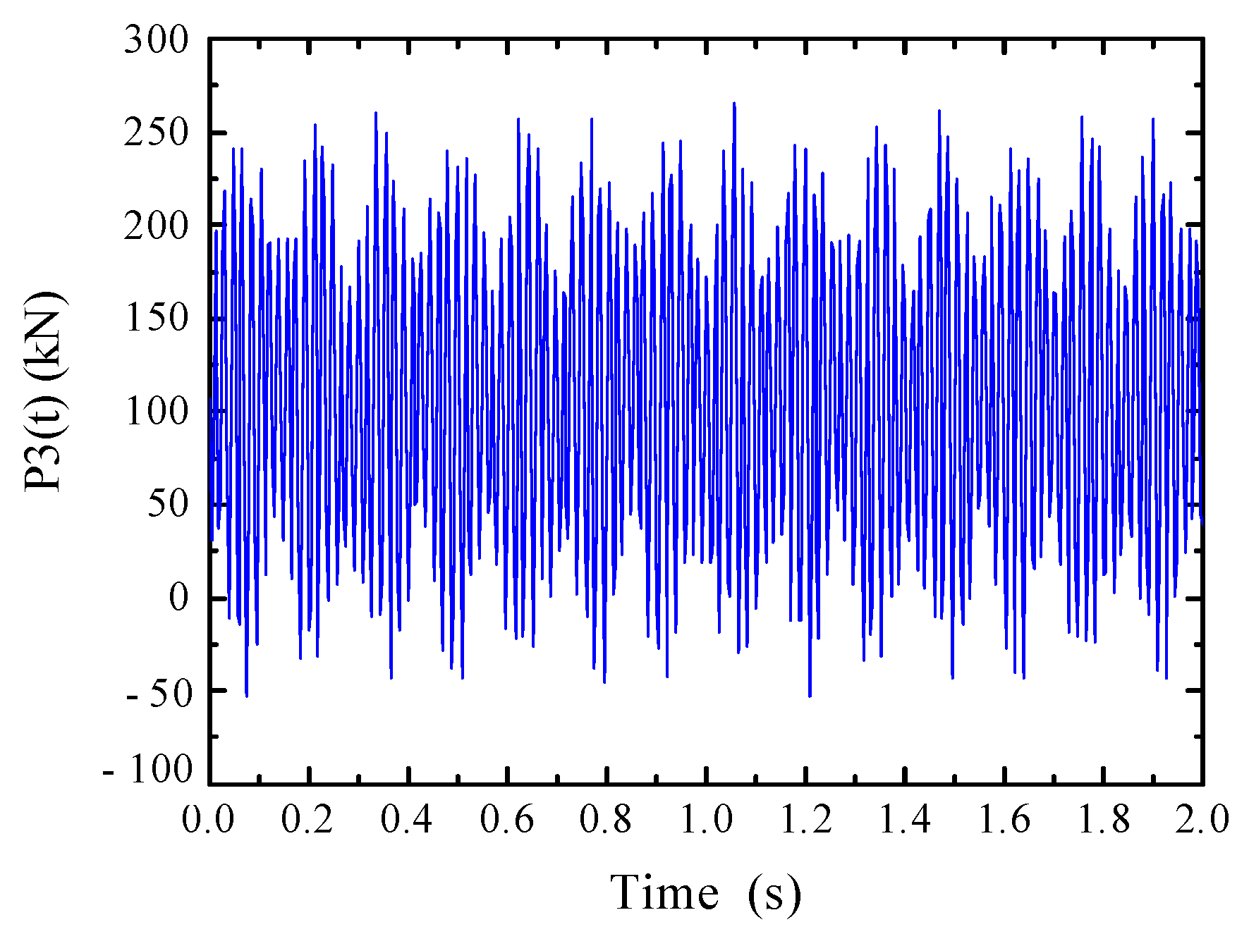
For the CRH380A high-speed train used in the model, the axle weight was 15 t and the unsprung weight was 750 kg. Considering the operating standards of high-speed railroads, train speeds are increasing; thus, the standards in
Table 2 have been adjusted appropriately and correspond to the wavelength and vector height in the three control conditions:
,
;
,
;
,
. The time–pressure curve of the vibration load at a train speed of 350 km/h was calculated and is shown in
Figure 5.
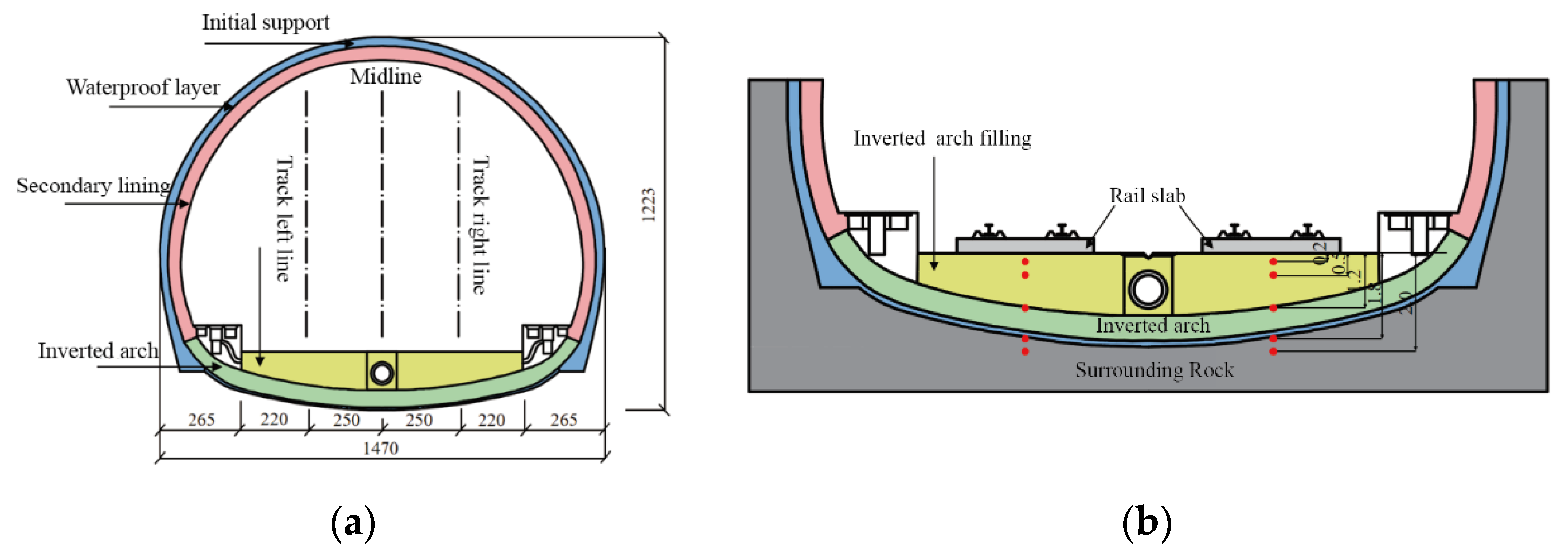
To verify the rationality of the determined empirical formula and numerical model, the decay law of the dynamic stress was verified. Because dynamic stresses measured in the field during passage of high-speed trains through a tunnel at speeds above 300 km/h could not be found in the literature, field measurements from sections of the Lanxin–Fuchuan high-speed railway tunnel were used to verify the numerical simulation. The train speed was 150 km/h; the tunnel cross-section of the high-speed railroad and arrangement of the pressure sensors are shown in
Figure 6.
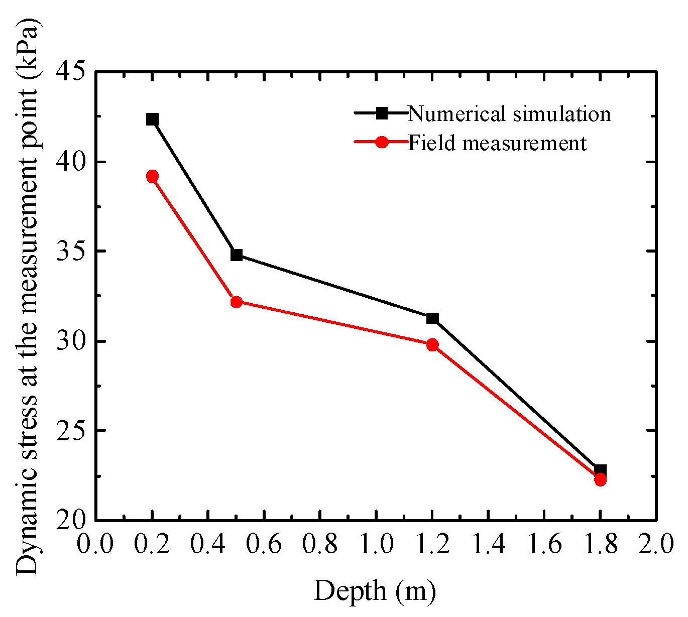
Figure 7 shows the decay curve of the dynamic stress below the track plate with depth at a train speed of 150 km/h. It was found that the field-measured values and the numerical simulation results had the same trend; with increasing depth, the deviations at different positions were 8.2%, 8.1%, 5.1%, and 2.2%. The deviation values were within 10%; thus, the numerical model and empirical formula were considered to be reasonable.
2.4. Analysis Process and Calculation Conditions
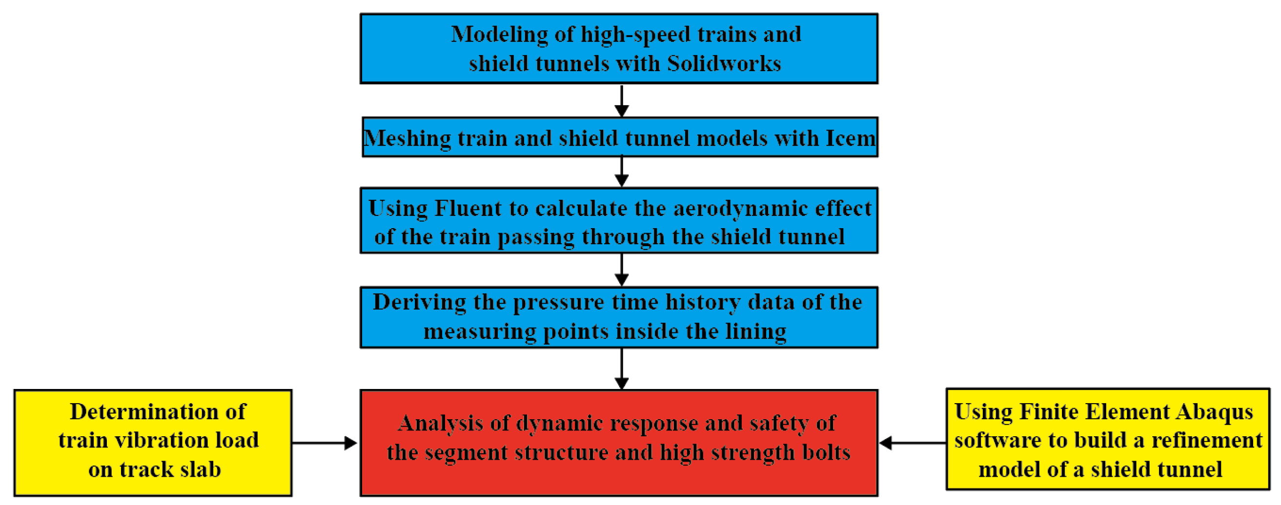
For the dynamic response of the segment structure and bolts with multi-field coupling during passage of a high-speed train through a tunnel, the time period of the aerodynamic load when the head and rear of the train pass through the measurement point was coupled with the vibration load to ensure that the results represent the most unfavorable condition. Using Fluent computational fluid dynamics software and ABAQUS finite element software, the dynamic response and safety of the segment structure and bolts with multi-field coupling were analyzed based on the model CRH380A high-speed train; the specific analysis process is shown in
Figure 8.
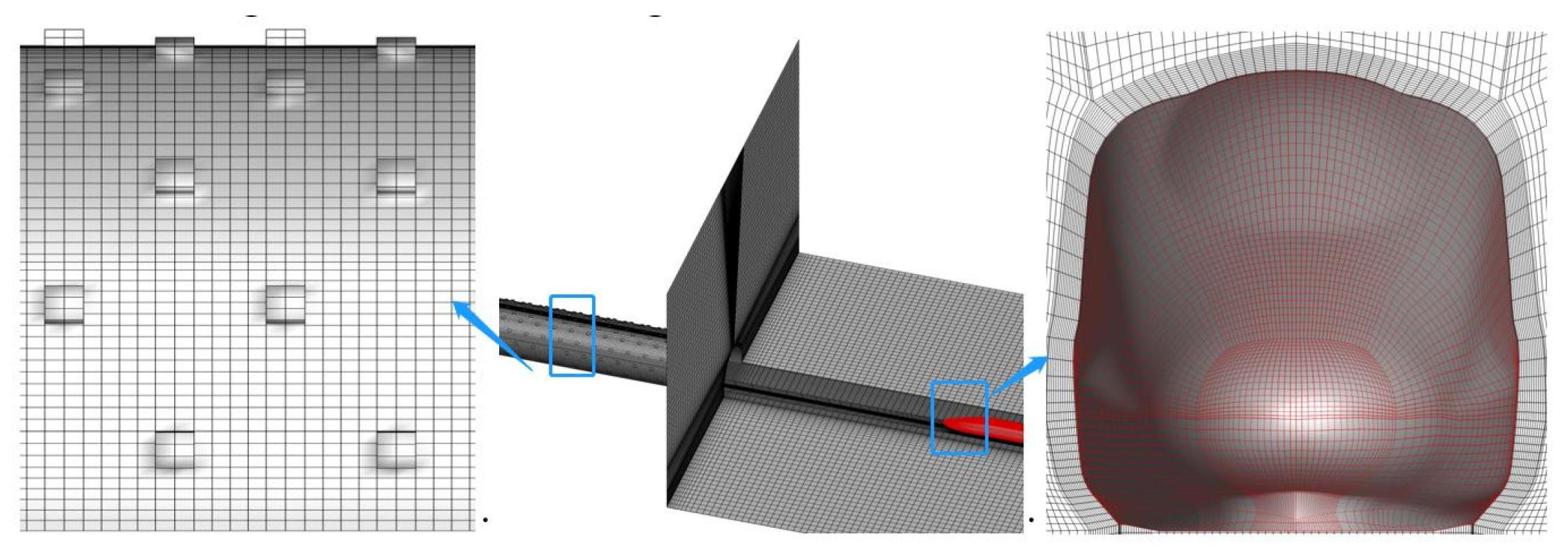
Solidworks software was used to establish the high-speed train and shield tunnel models (see
Figure 9 for details). Icem software was used to mesh the train and shield tunnel models. It should be noted that the bolt holes of the shield tunnel were simplified; see
Figure 10 for details. The divided mesh was imported into Fluent, the parameters were set, and the aerodynamic effects on the shield tunnel walls were calculated. The aerodynamic load at the most unfavorable location (the central monitoring point of the shield tunnel) was selected as the basis for analysis, and the train vibration load on the track slab was estimated using empirical formulas (see Formula (5)). With the established 3D finite element model, the calculated pneumatic and vibration loads (see the time–pressure curve in
Figure 4 and
Figure 5) were imported into ABAQUS in the form of a table in order to analyze the dynamic characteristics and safety of the segment structure and bolts in different working conditions (see
Figure 3b for details).
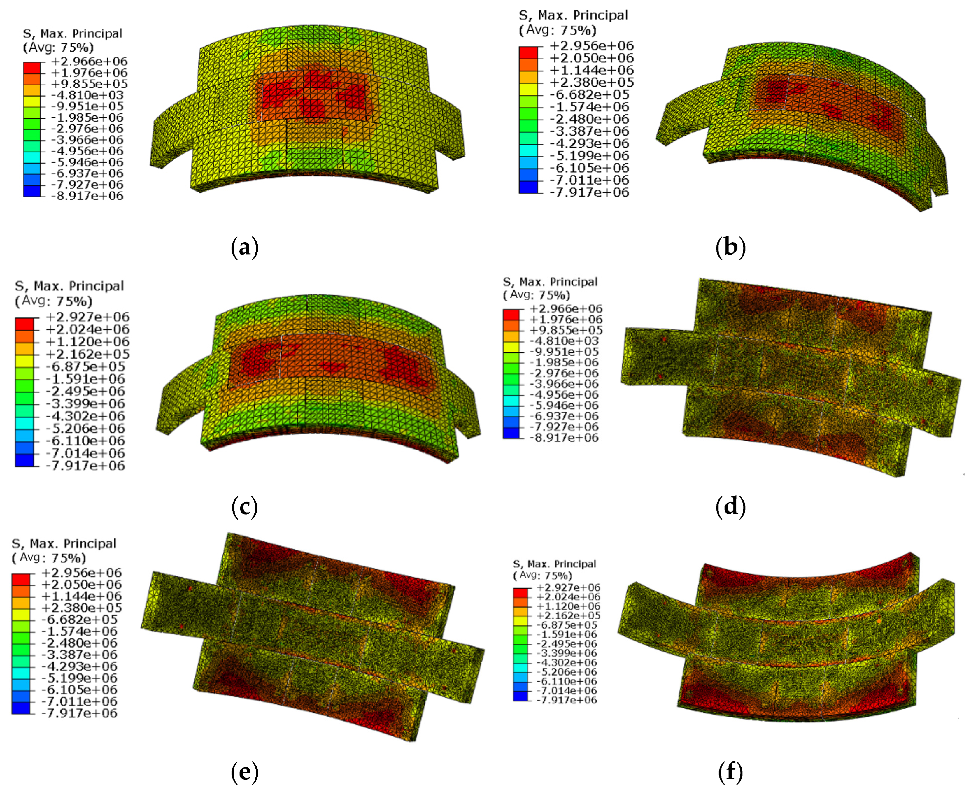
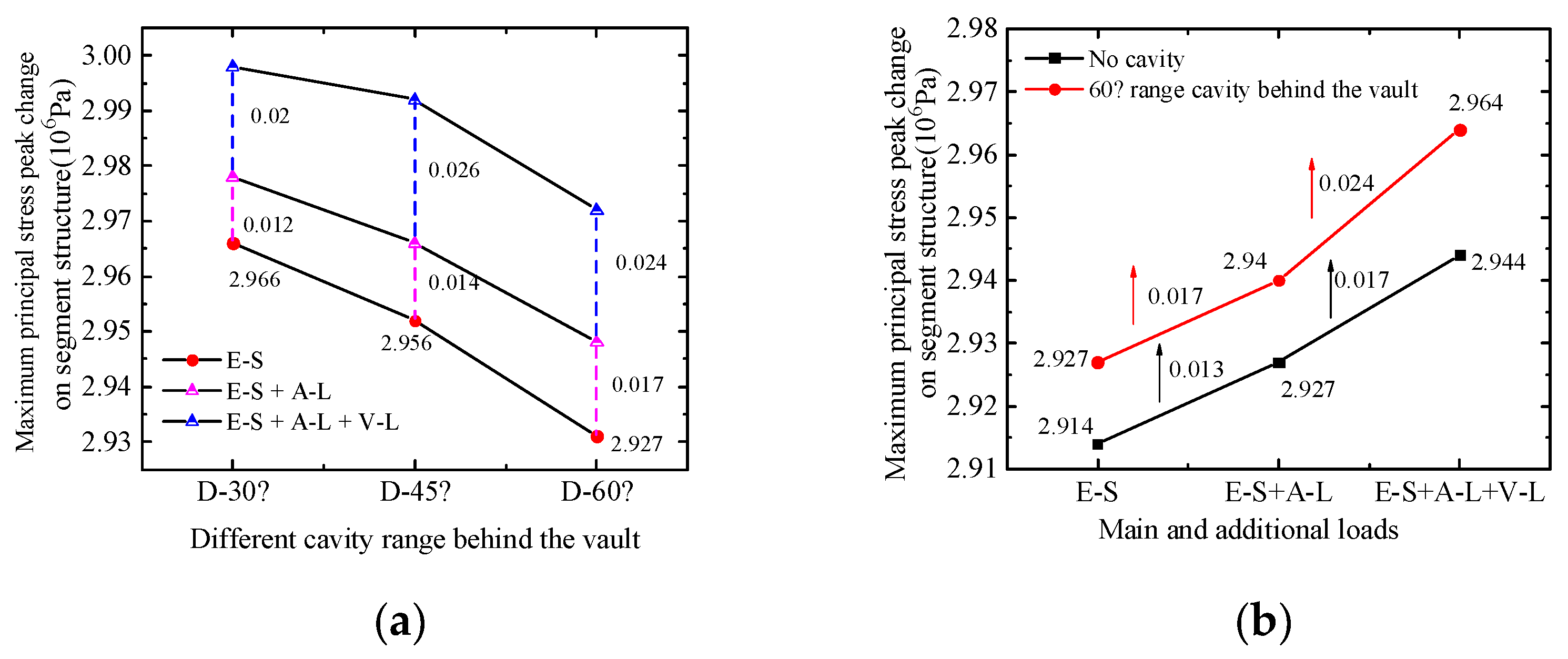
Table 3 presents the simulated working conditions for the finite element numerical calculations. For convenience of calculation, the effects of the cavity height and cavity length behind the lining were ignored; the cavity height and length in each working condition were defined as 0.5 m and 4.0 m, respectively. For A, with no cavity behind the segment, the debonding behind the vault was analyzed with the midline of the shield tunnel as the symmetry axis. The cavity range was 30°, 45°, and 60°, while the cavity area was symmetrical about the symmetry axis. The schematic diagram of the cavity scheme is provided in
Table 3. A1(A1′) and A3(A3′) are the edge measurement points at the junction position in the cavity and non-cavity areas of the segment, respectively, while A2(A2′) is the middle measurement point at the junction in the cavity and non-cavity areas of the segment. The letters outside and inside the brackets indicate the measurement points on the outer and inner sides of the segment, respectively. The same is the case for the other measurement points. For space considerations, only some of the measurement points behind the vault were analyzed.


