1. Introduction
Climate change and environmental pollution have been identified as being among the most significant challenges presently faced by humans. Commercial competition in the economic sphere combined with rising energy demand has exacerbated environmental threats. Only by transitioning to a sustainable built environment can we expect to achieve positive environmental outcomes. The term ‘built environment’ is a concept that broadly refers to the full range of structures that facilitate human activities [
1,
2,
3,
4]. More specifically, it denotes all physical forms that constitute a city, such as buildings, factories, transit systems, amenities, parks, and sidewalks [
4,
5,
6,
7]. Consequently, the built environment, as places where people live and work, greatly impacts human health and well-being. The built environment is also the principal driver of greenhouse gas emissions, which in turn is a cause of disease and illness in humans.
The built environment can be understood as a human-modified environment, where, along with buildings, supporting infrastructure sectors such as energy distribution, water supply, and waste management systems are present [
1,
2,
4,
8]. These sectors in particular account for a significant proportion of all natural resource consumption and greenhouse gas emissions [
1,
2,
4]. There is therefore a need for carbon-neutral energy sources. Among these are hydroelectric, generated by water power from dams, along with wind power generated by turbines and solar panels installed directly on residential, office, and commercial buildings. However, as things stand, the majority of available resources directed to the production of renewable energy for the built environment are also being depleted or destroyed.
Statistics compiled by the International Energy Agency (IEA) show that electricity production is responsible for 40% of the world’s carbon emissions, with the built environment accounting for more than a third of those emissions [
2,
8,
9]. Renewable energy technology (RET) strategies offer the promise of greatly reducing the environmental impact of buildings and other commercial and public infrastructure [
1,
2,
4,
5,
6,
9,
10]. In order to maintain a harmonious balance between nature and cities, built environments must be responsibly designed, planned, and constructed [
1,
2,
4,
5]. Recent studies have shown that considering the harmful environmental effects of fossil fuel-based production, the use of renewable energy sources, such as solar photovoltaic systems, wind turbines, waste and biomass, and concentrated solar power plants, can significantly enhance the sustainable development of the built environment. Ideally, buildings should be net producers of energy, independently fully generating their own use requirements. Similarly, all generated waste should be recycled.
While there is general agreement that ‘green energy’ is desirable and beneficial, it is less clear which sources of green energy—or ‘green growth’ strategy—are the most effective. Energy literally fuels the economic growth of all nations, but owing to environmental destruction and restrictions caused by the consumption of fossil fuels, countries need to adapt their energy consumption portfolio in ways that best support their economic growth [
11,
12,
13]. Therefore, countries need economic growth predicated on a mix of energy sources that optimizes sustainable development and minimizes environmental pollution while providing high economic outcomes.
‘Green growth’ is an identified strategy for countries to achieve sustainable development [
11,
12,
13,
14,
15,
16,
17,
18]. The concept of green growth has developed significantly over the past years. Initially, it was referred to as the ‘environmental industry’, but today, it is widely used to confront economic growth issues [
15]. Green growth affects not only the quality of growth but also impacts total production [
14,
15]. In its basic iteration, green growth is restricted to matters related to a low-carbon economy, but in broader discussions, it also embraces macroeconomic issues.
As understood by the OECD, green growth strengthens economic growth and development along with the continuous provision of well-being by way of natural assets [
19]. The UNEP, presenting a report titled ‘Towards a Green Economy’, consciously avoids describing green growth as a green economy [
15,
19]. In their view, green growth simultaneously increases income as well as human well-being, while also significantly reducing environmental risks [
15]. The World Bank also considers the concept as an effective vehicle for economic growth that simultaneously utilizes clean natural resources to produce energy while eliminating environmental pollution [
19]. In practice, the realization of green growth demands that dependence on fossil fuels be reduced in favor of renewable energy [
13]. Accordingly, reducing greenhouse gas emissions, through the substitution of fossil fuels with renewable energy, is valid both for developed as well as developing countries.
Forecasts suggest that if substitutions were realized, energy consumption around the world could be reduced by 36% by 2030, with annual emissions of polluting gases slashed by one-third, from 30 billion tons in 2010 to 20 billion in 2050 [
17]. Moreover, it has been estimated that only 1.25% of the world’s GDP would be required to support a full transition to renewable energy [
17]. Access for 1.3 billion people living in developing countries to clean and efficient energy by the end of 2030 is a stated UN objective [
15,
17].
The potential advantages of renewable energy are well documented. First, it reduces dependence on fossil fuels. Secondly, when traditional fuels experience price shocks, the availability of renewable energy serves to stabilize macroeconomic performance, thereby dampening price shocks in the fossil fuel market of the country [
14,
15,
16]. Thirdly, clean energy will facilitate improvement in energy efficiency, further leveraging long-term economic development. Fourthly, by improving energy efficiency and deploying renewable energy, nations can combat the challenges of environmental degradation [
14,
15,
18,
20]. Thus, renewable energies will not only reduce greenhouse gas emissions but will also bring economic growth. Specifically, research shows that if countries are able to increase their investment in clean energy and away from fossil fuels by 17% through to 2050, they will realize a saving of USD 112 trillion [
14]. The IEA estimates that decarbonizing the electricity sector will require an investment of USD 903 trillion from 2010 to 2050. The United Nations believes that replacing renewable energies in the nuclear sector alone requires an investment of USD 15 to 20 trillion [
14].
However, renewable energy also has its pitfalls, such as posing threats to biodiversity and animal life. Indeed, studies have identified green energy developmental paths as posing serious disruption effects to a variety of ecosystems [
14]. Therefore, it is necessary to evaluate the role of renewable energy technology in the greening of the economy. In this study, the impact of the deployment of renewable energy technology on green growth—and as a result, the reduction in CO
2 emissions and climate changes in developing and developed countries—is investigated. This is undertaken by evaluating the impact of the development of renewable energy technology on green growth, both in terms of the cumulative installed capacity of renewable energy, as well as by parsing the four key sectors of hydroelectric, wind, solar, and biomass.
This paper contributes to the literature on renewable energy technology capacities (RET) and green growth in the following ways:
Analyzing the impact of renewable energy technologies and policies on green growth in the built environment, covering 40 countries from 2010 to 2021.
Utilizing panel data estimators such as generalized least squares and generalized method of moments for robust analysis.
Identifying the varying contributions of renewable energy sectors to green growth in developed and developing countries.
Emphasizing the critical role of judicious renewable energy policies in stimulating investment and technological innovation for a sustainable built environment.
Carrying out a unique examination of how RET capacities mediate green growth, analyzed using multiple regression analysis on data from various sources including national energy statistics and policy reports.
The study is structured as follows.
Section 2 presents the theoretical relationships between RET and green growth.
Section 3 presents the research method and data, and describes the variables.
Section 4 presents the findings and discussion, while
Section 5 concludes the study.
2. Literature Review
The rising global energy demand presents serious environmental challenges for the future. This is the impetus for the development of renewable energy infrastructure, along with the promotion of clean energy use. However, in both developed and developing countries, the energy transition is expected to be both costly and time-consuming, not to mention technologically challenging. So far, green growth transitions towards reducing dependence on fossil fuels have been limited [
17]. Green growth literature emerged only as recently as the aftermath of the 2008 financial crisis, and then mostly in regard to developed countries. Green growth, however, has rapidly come to embrace such diverse concepts as employment, technology and innovation, and trade [
12,
14,
15]. Green growth, broadly conceptualized, is thus central to achieving sustainable development in assimilating both environmental sustainability and economic development [
13,
15,
16,
17,
18]. It has the potential to impart significant social as well as economic gains [
14]. Jouvet and De Perthuis (2013) [
21] believe that resource productivity, valuation of natural capital, and changes in energy systems, along with the pricing of external environmental effects, are facets that can be achieved with green growth.
Although most countries are amenable to green growth development goals, the specific green growth strategies pursued will vary from country to country [
22]. Between 2005 and 2010, investment in renewable energy increased by almost 40% annually. The installed capacities of solar PV grew by 72%, while wind grew by 27% [
15]. The concept of green growth has been placed center stage by many governments as a dominant political response to climate change and ecological collapse [
15]. Similarly, the growth in renewable energy markets has been accompanied by political feedback [
15,
22]. The dynamic interaction between government and green markets resulting from policy and innovative technologies has created a codependent cycle. Green growth theory asserts that continued economic development is compatible with our planet’s ecology for the reason that technological refinement and substitution allow us to decouple GDP growth from polluting fuel use [
12,
15,
17]. This claim is now mainstream thinking in national and international policy, including in the UN sustainable development goals [
11]. Given the established high social consciousness in regard to environmental protection, the concept of green growth now features strongly in the mindsets of both industrial and traditional societies [
11,
16].
A potent means by which to achieve green growth is to support the built environment’s transition to renewable energy. Numerous avenues have been explored in this regard. Systems of production and independent use of water and energy offer the possibility of significant resource consumption in residential areas [
1,
2,
5,
10,
23]. As investment costs in solar energy reduce, rooftop solar panels become an affordable alternative to serving household energy needs (e.g., lighting, television, heating and cooling, and kitchen use) [
6,
8,
9]. Additionally, emerging technologies even allow windows to generate energy under sunlight. In areas with sufficient humidity and rainfall, solar roofs can also be used to harvest rainwater (such as for bathing and washing) [
3,
7,
24]. Anaerobic digestion technologies can be used to produce biogas from domestic sewage, kitchen waste, and livestock waste [
2,
6,
23]. For example, organic and solid waste (paper, wood, and clothes) can be used to produce energy. Wood wastes along with other organic wastes can be used to improve soil performance, even in sequestering carbon for longer periods [
1,
4,
5].
According to the International Labor Organization (ILO), economic development based on renewable energy is expected to create 60 million jobs [
11,
16]. Renewable energy technology transition promises a significant contribution to the life and health of people, and to the alleviation of poverty. This is one of the main goals of green growth [
13,
17,
18], the aim being that the pursuit of new technologies will foster increases in productivity and lowering of energy costs as compared with traditional fuels [
15,
16,
17]. In developed economies, these technologies are emerging dynamically. However, in developing countries, which are heavily oil-reliant and innovation-poor, the installation of renewable energy technology capacities to support such projects is less visible [
15,
22].
In green growth, the existence of these capacities not only increases the strong presence of global markets and the private sector but also accelerates the development of innovative technologies [
15,
20]. Energy production from renewable energy sources has many advantages, especially for developing countries, because it reduces dependence on fossil fuels and stabilizes macroeconomic performance while preventing the transmission of oil price shocks [
16,
18]. Additional pollution can be reduced through advances in environmental technology. Granting subsidies to production enterprises, feed-in tariffs, and energy standard portfolios are among the policies that can take steps to preserve natural assets and reduce pollution [
13,
19,
20].
There are a few theoretical bases for assessing the role of green growth in protecting the environment. Hickel and Kallis (2020) [
17] showed that economic growth increases energy demand, leading to an increase in GHG, and undermining green growth. On the other hand, Hao et al (2021) [
16] investigated the role of green growth in environmental sustainability and found that not only is green growth strengthened by increasing energy consumption, but it also leads to a reduction in greenhouse gas emissions. Gasparatos et al (2017) [
15] believe that the use of renewable energy on a large scale will lead to green growth, but will have environmental consequences. The results of the research by Wiebe and Yamano (2016) [
25] state that to achieve green growth, demand-based greenhouse gas emissions are needed, which is possible through innovation in a cleaner production chain. For Umar et al (2020) [
26], green growth can be promoted through innovation in energy production, leveraged by environmentally friendly technologies. Guo and Ling (2017) [
27] show that green growth preserves natural resources and reduces CO
2 emissions, which can prevent environmental degradation. Lee (2011) [
28] also believes that green growth is necessary to achieve sustainable development since it has the potential to achieve environmental sustainability and economic development.
Smulders et al., (2014) [
22] called green growth a new concept and considered it a channel for establishing a connection between long-term investment in environmental protection and poverty reduction. They showed that there is no certainty in improving environmental impact and green growth. Sohag et al (2021) [
20] showed that investment interest rates have a negative effect on green growth. Menyah and Wolde-Rufael (2010) [
29] asserted that the move towards clean energy leads to the prevention of oil shocks in macroeconomic variables. For them, there is no specific relationship between green growth and environmental sustainability [
17]. Nevertheless, Strand and Toman (2010) [
30] envisage a positive and long-term relationship between green growth and environmental sustainability, as well as sustainable development.
Thus, it can be seen that the literature on green growth is extensive, and while overall sanguine as to the benefits, debate remains as to its efficacy with regard to particulars. Based on this, in the current research, we examine the variables of green growth, of which there are four key criteria. The first consideration is the relationship between economic growth and the use of natural resources. The second represents the risks to growth caused by any reduction in natural resources. The third is the environmental dimension of the quality of life, and how environmental conditions affect people’s well-being. The fourth dimension is the effectiveness of various governmental policies in catalyzing green growth. While the relevant extant literature includes green growth as a variable in studies, green growth has not been regarded as a dependent variable [
17,
20].
No study to date has examined the relationship between RET and green growth. In doing just that, our first contribution is in evaluating the role of RET in promoting green growth. Moreover, no previous study has identified the contribution of various installed energy capacities to green growth. Accordingly, this is our second contribution. Moreover, previous research in this area tends to be based on limited sample size; however, we have taken a wide sample set drawn from 20 developed and 20 developing countries, adding robustness to the findings.
3. Methodology
In this study, we investigated the relationship between the deployment of renewable energy technology and green growth in different countries. The approach taken is to compare the impacts of different variables drawn from a range of data sources. The variables used in this study include green growth (GE), total installed capacity of renewable energy technology (Ret), installed solar capacity (Solar), installed hydroelectric capacity (Hydro), installed wind capacity (Wind), installed waste capacity (Waste), renewable energy policies (Rep), population (Pop), consumer price index (Cpi), and emission index in million tons (Ghg). We used four main data sources to collect these data. The first source is the U.S. Energy Information Administration (EIA), the second source is Regulatory Indicators for Sustainable Energy (RISE), the third source is the World Bank’s World Development Indicators (WDI), and the fourth source is the Organization for Economic Co-operation and Development (OECD). A summary of the explanation of the variables showed in the
Table 1. In this study, the examined sample is divided into two categories of developing countries and developed countries, as listed in
Table A1. According to the International Monetary Fund, indicators such as government debt, real GDP, unemployment rate, consumer price index, and current account report were used to classify countries as developed and developing. From
Table 2 and the
Figure 1,
Figure 2,
Figure 3,
Figure 4,
Figure 5,
Figure 6,
Figure 7,
Figure 8,
Figure 9,
Figure 10 and
Figure 11, it is clear that there are different degrees of variation and expansion in RET and renewable energy installed capacity by sub-sector across countries. Differences in governance indicators, institutional development, economic systems, and geographic conditions are among the reasons for classifying countries into two categories, developing and developed, because these differences are expected to affect the effectiveness of RET as well as different sectors of this technology on green growth.
The present study uses the model proposed by previous research to investigate the effect of Ret on GE:
Here, Ret is the independent variable, i.e., the total installed capacity of renewable energy technology. It is examined both as a cumulative total, as well in four constituent sub-sectors: solar, hydroelectric, wind, and biomass [
31,
32]. Renewable energy policies are assessed using the World Bank’s Regulatory Indicators for Sustainable Energy (RISE, 2020), which provides a score between 0 and 100 for each country. A higher number indicates more efficient and effective renewable energy policies. Previous research, such as that by Eicke and Weko (2022) [
33], has used this variable as a proxy for clean energy support policies. That precedent is followed here.
GE is the dependent variable of the model in the present study, which indicates green growth. According to studies such as Azhgaliyeva et al (2019) [
34] and Hongo (2013) [
35], the variable production-based CO
2 productivity, GDP per unit of energy-related CO
2 emissions, is used as green growth. This study uses several data as control variables to analyze the impact of the deployment of renewable energy technologies (Ret) on green growth.
Population (Pop) is another important variable. As the population of a country increases, the need for energy consumption also increases. On the other hand, with an increase in population, the manufacturing sector of the country can utilize the growing labor force to expand green growth.
The Consumer Price Index (Cpi) is used as a proxy for energy prices in the model. This variable reflects changes in the ratio of household expenses to the average basket of consumer goods and services compared to a base year, set in this case to 2015. As used by Anton and Nucu (2020) [
36], this variable can be considered as a proxy for energy price in investigating the motivations of renewable energy producers to achieve green growth policies. Greenhouse gas (Ghg) emissions are another critical variable. According to several studies, the impact of dependency on fossil fuels to stymie green growth can be evaluated [
37,
38].
3.1. Cross-Sectional Dependency
The first step in choosing the appropriate panel unit root test is in detecting the existence of dependency between sections. Common unit root tests are presented assuming the absence of dependency between sections, while due to the existence of common characteristics and factors among members of a panel, there may be dependence between sections [
39]. Therefore, it is necessary to examine the cross-sectional dependency test first to determine whether the disturbances are cross-sectionally dependent or not. The cross-section dependence test used in this research was presented by Pesaran (2004) [
40]. In this test, the null hypothesis asserts the absence of cross-sectional dependence.
T is the time period, N is the sample size under investigation, and is the estimate of the cross-sectional correlation of the errors of countries i and j.
3.2. Slope Homogeneity
The next step is to reveal the slope homogeneity between the cross-sections. Ref. [
41] proposed the slope homogeneity test by considering the homoscedasticity assumption. The Swamy test is applicable for small panel data. The [
42] test is another method to examine slope homogeneity for large panels. The improved [
41] test formed two deltas. The slope heterogeneity among the countries in the panel will be showed by a large chi-square statistic.
: number of cross-section units, : Swamy test statistics, k: independent variables.
The null hypothesis posits that cointegrating coefficients are homogeneous.
3.3. Unit Root
In the next step, the stationary of the variables should be tested. Some variables are nonstationary due to cross-sectional dependency, which can lead to invalid results in model estimation. Therefore, the unit root test should be performed. There are two types of unit root tests. The first assumes the absence of cross-sectional dependency, while the second performs the unit root test assuming the presence of cross-sectional dependency. In this study, we used CIPS. Due to the cross-sectional dependency problem, Pesaran (2007) [
43] suggested that the normal ADF be modified [
44], as follows:
The unit root test [
43] is based on the average augmented ADF statistic in the cross-section. Pesaran (2007) explained the augmented version of the IPS unit root test as follows:
CADF indicates the cross-sectional augmented Dickey–Fuller statistic for each cross-section. In this method, the null hypothesis indicates the existence of nonstationary variables.
3.4. Cointegration
Due to the presence of nonstationary variables in the model, the results obtained from the estimation may be invalid. Thus, the cointegration between the variables must be checked. The presence of cointegration indicates the possibility of a long-term equilibrium relationship between the variables. There are different types of cointegration tests in order to scrutinize the long-term relationship between variables, such as [
45] and [
46]. In this research, Westerlund (2007) [
46] is used to determine cointegration, having been described as more accurate than Pedroni’s test [
44].
Due to the strongly balanced data in the research, we used the [
45,
46] tests to investigate cointegration. Unlike the [
45] test, which is based on the error component, the [
46] is a structure-based test that is more accurate than the Pedroni test. Pedroni is another method to clarify the long-term relationship between variables. The null hypothesis illustrates the absence of the cointegration relationship.
The Westerlund test uses the error correction model to confirm the presence of cointegration. The null hypothesis in this test indicates no cointegration. This test is designed on the basis that the null hypothesis of no cointegration is tested according to whether the error correction component in the conditional error correction model is equal to zero or not. Therefore, the rejection of the null hypothesis based on the lack of error correction can indicate the rejection of the null hypothesis based on the absence of cointegration.
In the above equation, dt contains definite components, Yit indicates the dependent variable (in this research, green growth), and Xit indicates the explanatory variables of the model, such as the installed capacities of renewable energy technology. In this equation, and the parameter 𝛼i indicates the adjustment speed of the system towards long-term equilibrium after a sudden shock. If the relationship is established as , the model is error correction, and it indicates that Yit and Xit are cointegrated. If , there is no error correction and therefore, there is no long-term relationship.
3.5. Feasible Generalized Least Squares
Based on previous studies such as Khan et al (2019) [
38], we used a logarithmic function for variables. The logarithmic use of variables in the model leads to more accurate results.
In this equation, β
0 represents the intercept.
β1,
β2, …
β8 represent the coefficients of explanatory variables of the model, where the meaning of each is the β percentage increase or decrease in the variables on the right side of the model, which determines percent increases or decreases in the dependent variable, i.e.,
GE. ε also represents the disturbance component of the model. FGLS is an estimator used in the incidence of heteroskedasticity, CD, and panel serial correlation. When problems such as serial correlation and variance heterogeneity appear in the research variables, the use of the generalized ordinary least squares method is more efficient than the ordinary least squares method [
38].
The specification of a simple ordinary least squares model is expressed as follows:
Y is the dependent variable,
X is the independent variable (explanatory), and
ε is the error disturbance of the model. If there is heteroskedasticity or a lack of autocorrelation in the model’s error disturbance, Gauss Markov conditions are violated. In this way, the ordinary least squares model cannot be used. Therefore, we assume:
is a symmetric matrix that includes assumptions related to serial correlation, CD, and heteroskedasticity. Thus, we can write Equation (10) as follows:
We can say:
Now, we can use the generalized ordinary least squares estimation.
3.6. Generalized Method of Moments
Based on previous studies such as Moradbeigi and Law (2016) [
47] and Nili and Rastad (2007) [
48], the following equation is used to estimate the model.
Z is the vector of control variables.
In any estimation of a model with panel data, we must first check whether
is a fixed effect or a random effect. Using the random effect method in Equation (15) is not suitable, because the hypothesis of no relationship between the explanatory variables and the effects of the sectors is rejected. On the other hand, the fixed effect method is ineffective for solving the endogeneity problem. Therefore, we introduced a two-stage least squares model (2SLS) and the generalized moments model (GMM), which can be used to solve the correlation problem between the explanatory variables of the model and error disturbance [
49,
50]. Another advantage of this method is the ability to solve problems such as serial correlation and heteroskedasticity.
GMM is divided into two groups: system [
51] and difference [
50]. Regarding difference, the lag of the dependent variable is used as an instrument at the level [
50]. Blundell and Bond (2000) [
51] and Bound et al (1995) [
52] believe that the use of a lag variable in the level is a weak tool for the model, which is why the system method is used. Note that the relationship between the lag of the dependent variable (
) and the specific random component of the section (
) can make the estimator inconsistent; thus, we can remove the influence of the fixed effect from the model by considering a first-order difference.
Δ is the first-order difference operator.
Due to the existence of a correlation between the specific disturbance component of the model (
) and the lag of the dependent variable (
), the ordinary least squares model cannot be used due to the bias and inconsistency that is created. Therefore, Arellano and Bond (1991) [
52] proposed the generalized method of moments. Moreover, in this model, the lag of the dependent variable (
) can be used as a tool, which is the first-order difference.
However, Bound et al. (1995) [
52] stated that this tool cannot be used as an efficient tool in the first-order difference model due to it being nonstationary. For this reason, we adopted a different form to solve this problem [
53]. The solution was to use the lag of the dependent variable in the matrix of instrumental variables. This method is the same as the generalized moments of the system. In this study, the two-stage method of the system is used. In the simulation results of the model, if the dependent variable coefficient is closer to one, the system method will be a more accurate estimator [
47].
The compatibility of the generalized method of moments estimator is due to the lack of serial correlation of the error component and the validity of the tools. This compatibility is achieved using two tests [
53]. The first is the M2 statistic, which tests the existence of the second-order serial correlation in the first-order differential error component. Failure to reject the null hypothesis in both tests provides the assumption of serial non-correlation and validity of the instruments. The second is the Hansen and Sargan test, which has predetermined restrictions that determine the validity of the instruments. In this test, by not rejecting the null hypothesis, we conclude that the selected instruments are valid.
4. Results and Discussion
First, we examined a statistical description of the variables used in the current study. Then, we evaluated Pesaran’s cross-sectional dependency test, followed by the stationary test, and finally the cointegration test. Descriptive statistics are presented in
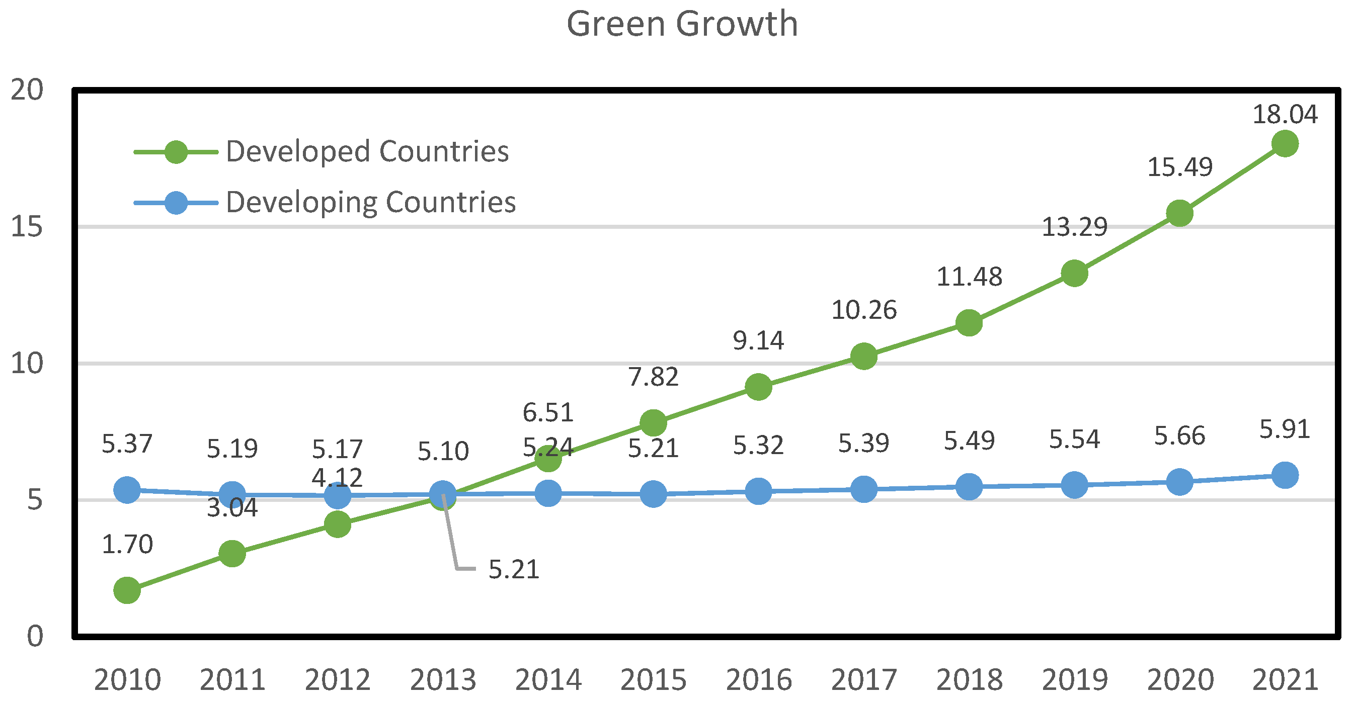
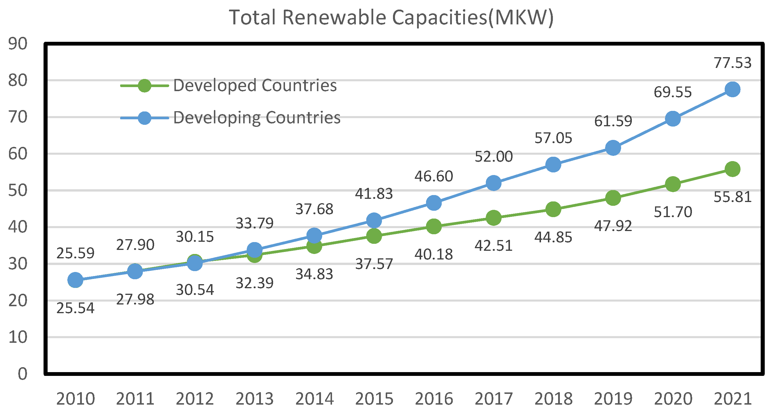
Table 2. All the numbers in the table are natural logarithms. According to this table, the rate of green growth is higher in developed countries than in developing countries. For developed countries, the maximum is 2.88 and the minimum is 0.91, with an average of 1.81. For developing countries, the maximum and minimum are 2.77 and 0.39, respectively. Countries with the highest RET capacity are developing countries with 6.92 units and an average installation of 2.35. For developed countries, these numbers are 5.79 units and 3.05. The lowest installed capacities for developing countries and developed countries were −1.30 and 0.59, respectively.
These statistics highlight a counterintuitive result. That is, the results for some sectors of the installed capacity of renewable energy for developing countries are higher than in developed countries. According to the EIA database, we observe that China has a vast installed capacity of renewable energy. This signals its advanced developmental status, yet according to the classification of countries tabled by the IMF, China remains classified as a developing country [
54].
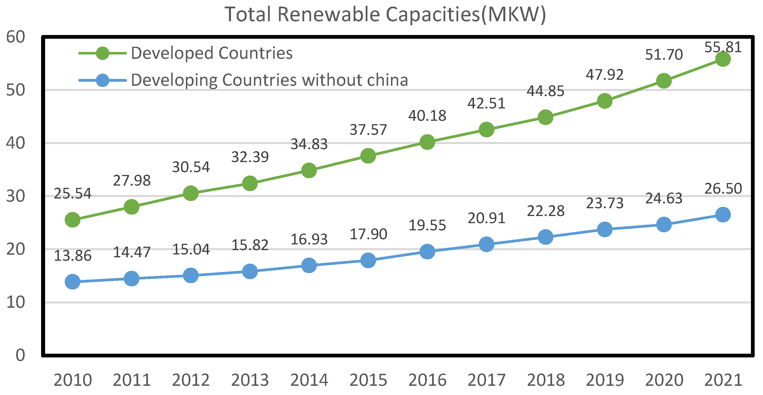
Thus, we need to adjust comparisons to address the China anomaly. Consequently, two groups were extracted. The first group comprises a comparison between developing and developed countries, as defined by the IMF, while the second group is a comparison without the presence of China. In so doing, we can develop a clearer understanding of China’s influence on the data of developing countries.
Table 3 shows the results of the Pesaran’s (2004) cross-sectional dependency test for the variables. Statistics related to each variable along with their probabilities are presented in parentheses. According to the table, our null hypothesis of independent of sections is rejected at the 1% level. As can be seen, the results show that there is a dependency of sections in all variables. Moreover, according to
Table 4, we conclude that the null hypothesis is rejected; therefore, panels have slope heterogeneity.
According to the observations in the cross-sectional dependency test, in which variables are affirmed to be cross-sectionally dependent, we used the second generation of tests [
43] to test the stationary status of the research variables. The results of
Table 5 show that all panels are stationary, either at their level or in the first-order difference.
The presence of stationary variables shows the necessity of using the second-generation cointegration test, as described by Westerlund (2007) [
46] and Khan et al. (2019) [
38]. This test is suitable for examining the long-term relationship between variables with cross-sectional dependencies [
37].
Table 6 and
Table 7 present the results of the cointegration test. The statistics show that the null hypothesis of no cointegration in all panels is rejected, which indicates the existence of a long-term relationship between these variables.
In the estimation of economic models, it is not recommended to use a large number of variables due to the degree of freedom restriction, as this can decrease the validity of the regression and reduce the R2 statistic. Moreover, these five variables fall under the same classification, indicating strong collinearity between them. The presence of collinearity can increase the confidence interval for the significance of the coefficients, potentially leading to biased results such as invalid coefficients.
The results of
Table 8 and
Table 9 show that the RET coefficients are positive and significant. This indicates that the RET index has a positive effect on green growth (GE) in both developed and developing countries. For example, based on the GLS model in
Table 8, a 1% increase in the RET index in developed countries will result in a 0.07% increase in green growth. For developing countries, this will result in a 0.08% increase. At the level of 1%, these coefficients support the proposition that the countries of this study have been successful in achieving green growth by installing increased capacities of renewable energy. Specifically, we see that support for clean energy leads to the formation of improved energy-efficient industries that spur green growth through economic growth.
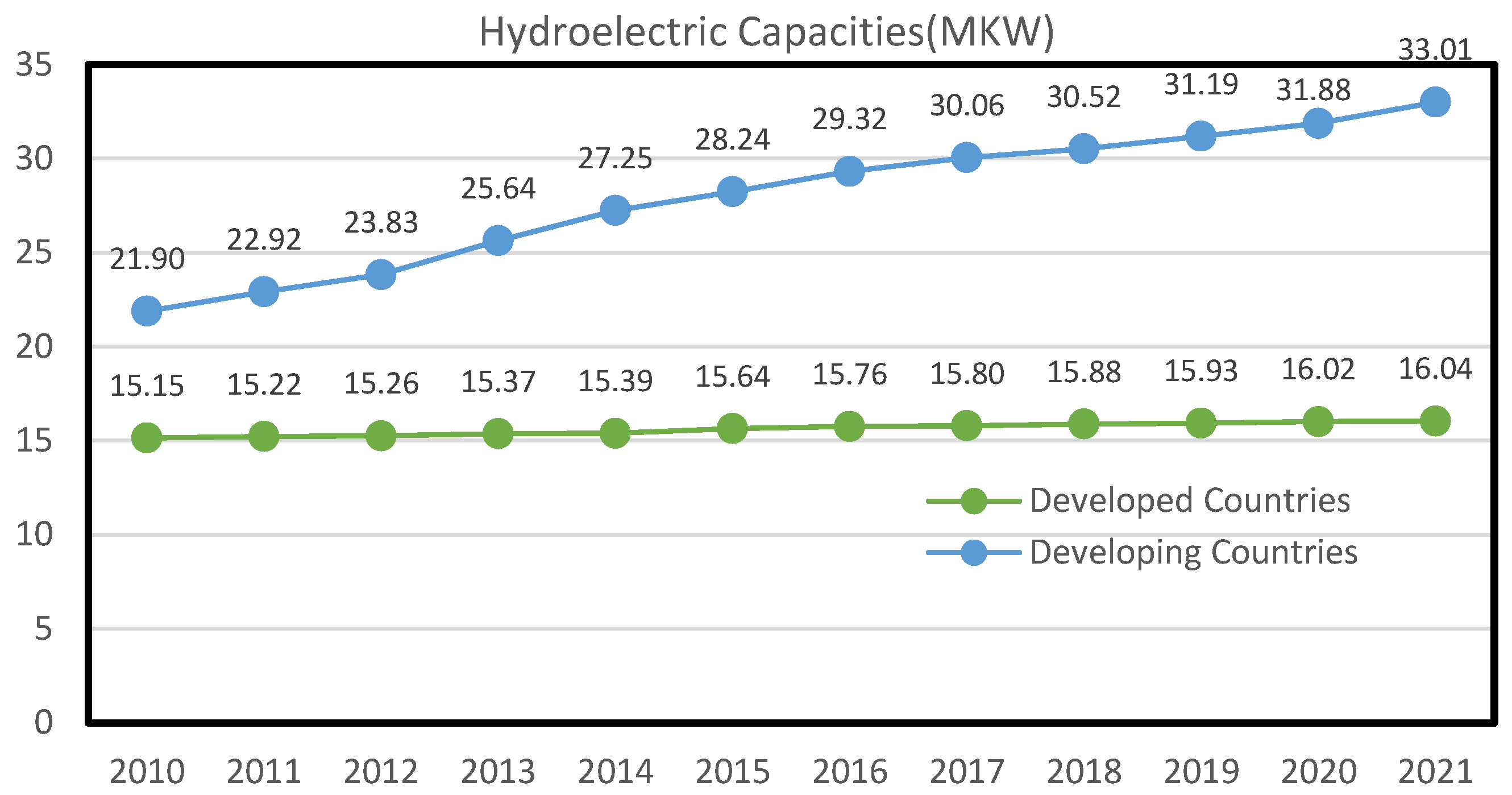
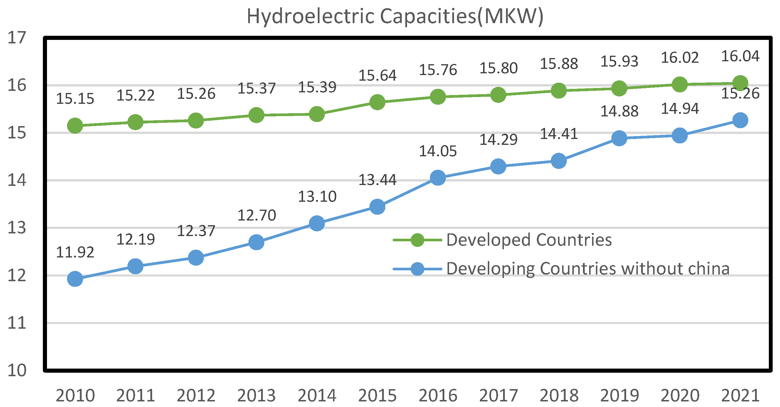
Each sector of total renewable energy capacity was also assessed. According to the GLS model, installed hydroelectric capacity in developed countries has not had a positive impact on green growth. As we see in
Figure 1, the amount of installed hydroelectric capacity has not significantly increased over the study period. However, in the GMM model, at the level of 10%, this effect was positive and significant. Other capacities have had a positive and significant impact on green growth.
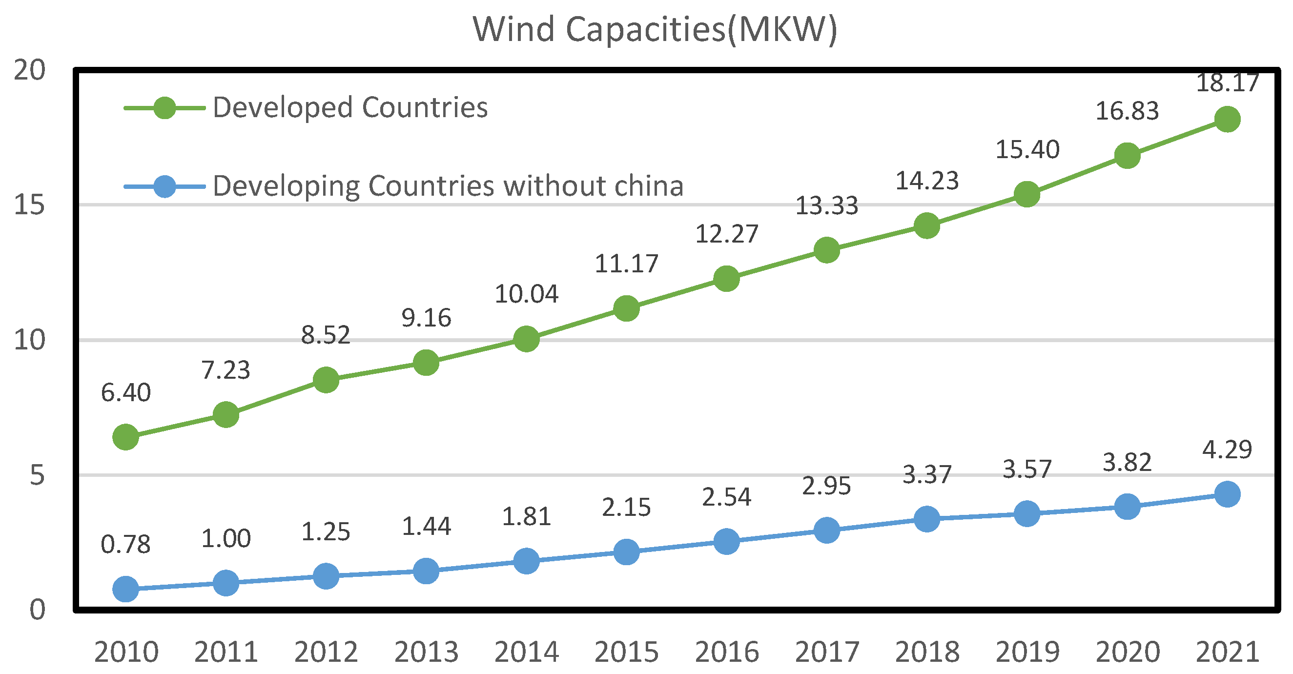
In developing countries, the installed capacities of wind both in the GLS model and in the GMM model did not stimulate green growth, but other capacities did facilitate the expansion of green growth. Overall, we can see that the size of the formation of green growth arising from renewable energy capacities is higher in developed countries than in developing countries. Developed countries mostly have abundant accessible natural resources. Vital resources such as underground aquifers due to rainfall, dense forests, and suitable geographical locations create conditions for these countries to extract advantages in the deployment of renewable energy, as compared with developing countries.
In addition, the existence of government support policies such as financial incentives and their effective implementation has led to the further development of green growth. However, increased banking activities and more effective financial markets in developed countries, compared to developing countries, allow more effective transfers of capital flow from traditional energy projects to green growth projects. In developed countries, the renewable energy market has led to green growth as a consequence of the strong presence of the private sector and the lack of government interference. Therefore, it can be said that due to privatization in these countries, most renewable energy projects, such as the provision of innovative equipment, are well supported. In developing countries, the existence of greater financing challenges experienced by enterprises, combined with heightened investment risk, results in a smaller scale of green growth through renewable energy.
The low cost of fossil fuels and the quick returns such projects offer lead to persistent dependence on them. Therefore, enterprises resist renewable energy policies where they can. Thus, as can be seen from the results, it is clear that renewable energy policies have not been able to shape green growth. Population growth, on the other hand, has been able to support green growth. Such growth facilitates a labor force with the knowledge to support green growth policies with clean products. It can be argued that improving the quality of human capital through investment and education can create awareness among the population about the use of environmentally friendly technologies.
The Cpi variable, according to the results of the GLS method, had a positive effect on green growth, but according to the results of the GMM method, it had no effect. Thus, it remains unclear whether an increase in prices will motivate producers to pursue green growth. A portion of national GDP comprises oil rents, and as a result, the coefficient of greenhouse gases shows that dependence on fossil fuels is a factor in these countries. In the early stages of development, countries focus on manufacturing activities and hence emit more greenhouse gases. However, once they reach a certain level of development, countries focus on improving environmental quality and hence use environmentally friendly technologies in the effort to reduce CO
2 emissions in the long run. Simply, people worry first about improving their economic outlook, and it is only when a threshold level of economic prosperity is achieved that citizens of a country will cast their minds to the greater good of the nation, its environment, or its future legacy.
Table 8 and
Table 9 show that in the FGLS and GMM methods, the Wald statistic indicates the validity of the regression, and due to the high numbers, the null hypothesis of the insignificance of this coefficient is rejected. However, in justifying the statistics (AR 1) and (AR 2), the Sargan test, as mentioned in the explanation of the GMM method, indicates a lack of serial correlation between the error component and the validity of the instruments. Unlike the significance of the coefficients of variables such as population, where the probability of the statistic must be less than 0.05, in these statistics, the probability must be greater than 0.05 to confirm the null hypothesis of the absence of serial autocorrelation and the validity of the instrumental variables.
5. Conclusions
The purpose of this study is to investigate the impact of renewable energy installed capacities, renewable energy policies, population, consumer price index, and greenhouse gas emissions on green growth. Two groups were compared, comprising developed and developing countries. The timeframe from which comparisons were drawn was 2010 to 2021. In summary, the results indicate that the impact of renewable energy installed capacity differs according to a country’s developmental status. Developed countries have more capacity to support green growth than developing countries. This is due to the greater efficiency exhibited in their renewable energy policies. In developed countries, renewable energy policies have a greater capacity to stimulate investors and scientific enthusiasm in furthering renewable energy technological capacity. In turn, this can be attributed to the incentivization of the private sector and financial institutions to finance such projects. As a result, direct capital flows towards productive activities such as importing equipment related to renewable energy projects occur. By comprehensively supporting production and economic growth, developing renewable energy capacities, and effectively integrating industry and households, a dynamic economy can be created. It is possible to raise the attractiveness of investment in renewable projects through policies such as tax credits, subsidies, and grants. These mechanisms serve to cap energy pricing at acceptable market rates. The result is a reduction in the cost of renewable energy technologies, reduced pollution, increased energy efficiency, and a lowered poverty index, all of which constitute green growth policies.
Green growth and eco-innovation are facilitating a change in the industrial structure from non-renewable to renewable energy sources, and consequently alleviating CO2 emissions. In addition, green growth is seen as an important strategy for achieving sustainable development. Environmental pricing through taxation is likely to stimulate cost-effective and environmentally friendly means of production while discouraging activities that stimulate CO2 emissions. Similarly, environmental taxes lead to shifts in investment and consumption behavior. Moreover, developed human capital is a prerequisite for the successful implementation of these policies. Improving the quality of human capital through investment and education can create awareness in society regarding the use of environmentally friendly technologies.


