Prediction of Ultimate Bearing Capacity of Pile Foundation Based on Two Optimization Algorithm Models

Abstract

The determination of the bearing capacity of pile foundations is very important for their design. Due to the high uncertainty of various factors between the pile and the soil, many methods for predicting the ultimate bearing capacity of pile foundations focus on correlation with field tests. In recent years, artificial neural networks (ANN) have been successfully applied to various types of complex issues in geotechnical engineering, among which the back-propagation (BP) method is a relatively mature and widely used algorithm. However, it has inevitable shortcomings, resulting in large prediction errors and other issues. Based on this situation, this study was designed to accomplish two tasks: firstly, using the genetic algorithm (GA) and particle swarm optimization (PSO) to optimize the BP network. On this basis, the two optimization algorithms were improved to enhance the performance of the two optimization algorithms. Then, an adaptive genetic algorithm (AGA) and adaptive particle swarm optimization (APSO) were used to optimize a BP neural network to predict the ultimate bearing capacity of the pile foundation. Secondly, to test the performance of the two optimization models, the predicted results were compared and analyzed in relation to the traditional BP model and other network models of the same type in the literature based on the three most common statistical indicators. The models were evaluated using three common evaluation metrics, namely the coefficient of determination (R²), value account for (VAF), and the root mean square error (RMSE), and the evaluation metrics for the test set were obtained as AGA-BP (0.9772, 97.8348, 0.0436) and APSO-BP (0.9854, 98.4732, 0.0332). The results show that compared with the predicted results of the BP model and other models, the test set of the AGA-BP model and APSO-BP model achieved higher accuracy, and the APSO-BP model achieved higher accuracy and reliability, which provides a new method for the prediction of the ultimate bearing capacity of pile foundations.

1. Introduction

As a structural element that transfers the load applied by a building to a certain depth underground, a pile foundation has a high bearing capacity, wide application range, and long history. Due to their unique advantages, pile foundations are widely used, and their structural types are also developing towards diversification. However, due to the interaction between pile and soil, the behavior of a pile under load is very complex. How to determine the ultimate bearing capacity of a pile foundation scientifically and reasonably is a key technical issue in pile foundation design.

Many of the available experimental or theoretical methods for predicting pile bearing capacity contain assumptions about the parameters of governing ultimate bearing capacity, which simplify such issues as the cone penetration test (CPT) [1], dynamic load test (DLT) [2], standard penetration test (SPT) [3,4], and static load test (SLT) [5]. Therefore, the most direct and reliable method for determining the bearing capacity of a pile is still to load the pile statically until its failure. The static load test (SLT) and high strain dynamic load test (HSDT) are two common methods for estimating the bearing capacity of pile foundations [6]. However, considering the cost of testing, it is necessary to reduce the number of tests, which means that it is also necessary to find a more efficient and accurate new method to predict the bearing capacity of pile foundations.

In recent years, information technology has developed rapidly in civil engineering and has been used to solve geotechnical engineering issues; in particular, the use of machine learning methods to solve different aspects of practical engineering has received increased attention [7]. Essentially, machine learning is a combination of mathematics, algorithms, and creativity, and it contains support vector machines (SVMs) [8,9], artificial neural networks (ANNs) [10,11], an adaptive neuro-fuzzy inference system (ANFIS) [12,13], and other techniques. Many scholars have applied these techniques to predict the bearing capacity of pile foundations. Baginska and Srokosz [14] conducted a large number of network experiments to predict the bearing capacity of shallow foundations and pointed out that between five and seven layers in a neural network are the best number to predict the bearing capacity of a shallow foundation. Karimipour et al. [15] used neural networks to predict the bearing capacity of concrete columns under axial loads and obtained results with relatively high accuracy. Alzo and Ibrahim [16] used a back-propagation (BP) method algorithm and general regression neural network (GR-ANN) to reasonably predict the static load experiment, verifying the mode with the existing experimental data. The results show that, based on the same quality and quantity of data, the BP algorithm obtains better results than the GR-ANN, proving the feasibility of using a BP neural network to predict the ultimate bearing capacity of pile foundations. However, all the above methods only use a single network model, and the prediction accuracy is expected to improve compared to the hybrid model.

The BP neural network, which is widely used in a single model, is relatively mature in performance and theory; however, due to the randomness of its initial weight and threshold, there are still some shortcomings, such as system instability, ease of encountering a local minimum problem, and slow convergence speed [17]. Considering these issues, many scholars have proposed optimization methods to improve the performance of a single network. Luo et al. [18] used a genetic algorithm (GA) to optimize a BP network training algorithm to improve accuracy. Zhang and Li [19] applied a particle swarm optimization (PSO) algorithm to optimize the topological structure of a BP network. Saffaran et al. [20] used an annealing algorithm to optimize the weights and thresholds of a BP network. Furthermore, Momeni et al. [21] developed a GA-based ANN model; the pile group, the cross-sectional area and length of the pile, the hammer weight, and the drop hammer height were taken as the input parameters, and the ultimate bearing capacity of the pile was taken as the output of the network model. The results obtained demonstrate the applicability of the model as a feasible and effective tool for predicting the bearing capacity of pile foundations. Singh and Walia [22] used four natural heuristic algorithms to establish the correlation coefficient: particle swarm optimization, fire flies, cuckoo search, and bacterial foraging, and two trained artificial neural networks were used to determine the frictional force of the unit surface and the bearing capacity of the pile end according to the soil properties. Compared to ANN, PSO is less time-consuming and less complex, and it is the best performer in solving such constrained issues. According to the predicted results of various machine learning methods in relation to the ultimate bearing capacity of pile foundations in the literature, the PSO algorithm and GA algorithm show a better predictive effect in this kind of prediction model. It is worth studying how to scientifically and effectively predict the vertical bearing capacity of a pile foundation, effectively combine various influencing factors that cannot be expressed by a precise formula through a neural network and obtain a relatively accurate predicted result according to the prediction model, so as to grasp the overall quality of the pile foundation construction of the whole project.

Most of the current prediction methods of ultimate bearing capacity of pile foundations use a single prediction model or a simple combination of two algorithms; although the predicted results can provide some reference for construction design, their accuracy is expected to continue to improve. Based on this situation, this study proposes two optimization algorithms for predicting the ultimate bearing capacity of a pile foundation; by modifying the genetic algorithm and particle swarm optimization evolutionary iteration, the algorithm can independently select a suitable parameter to continue in the process of operation, thus greatly improving the accuracy of prediction. According to the analysis of influencing factors in several references and the collected data, seven factors were found to be related to the ultimate bearing capacity of the pile foundation: selecting pile length (L), pile area (A), pile type (T), pile side soil cohesion (C), internal friction angle ($\mathsf{\phi }$), pile side soil standard penetration hammer number (N), and ultimate end resistance of pile end soil ($q_p$). These were selected as the input parameters of the network model, and the vertical ultimate bearing capacity of the pile foundation was taken as the output parameter of the model. The performance of the network model was evaluated by three commonly used evaluation indicators; namely, the determination coefficient (R²), value account for (VAF), and root mean square error (RMSE), and the predicted results of other network models of the same type in the literature were compared and analyzed. The BP neural network optimized by the adaptive genetic algorithm (AGA-BP) and the BP neural network optimized by adaptive particle swarm optimization (APSO-BP) proposed in this article achieved good results, and the predicted results of APSO-BP were more accurate, which provides a new method for the prediction of the ultimate bearing capacity of pile foundations.

2. Prediction Method of Ultimate Bearing Capacity of Pile Foundation

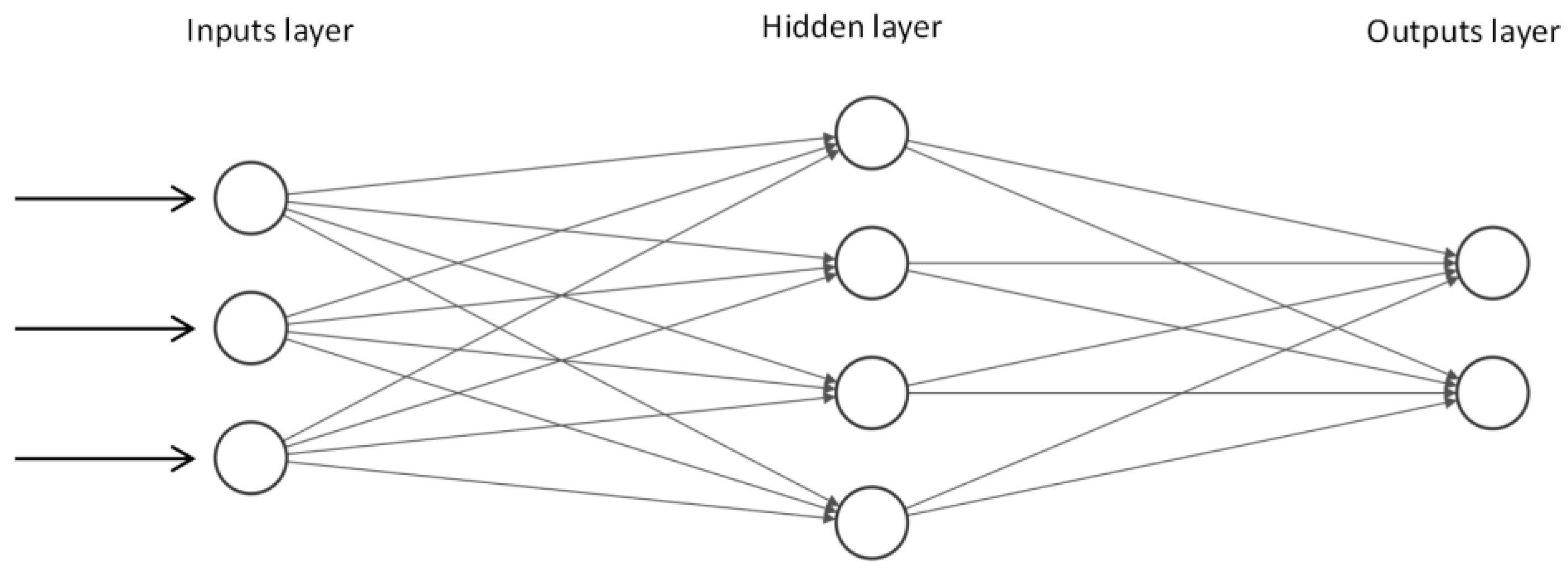
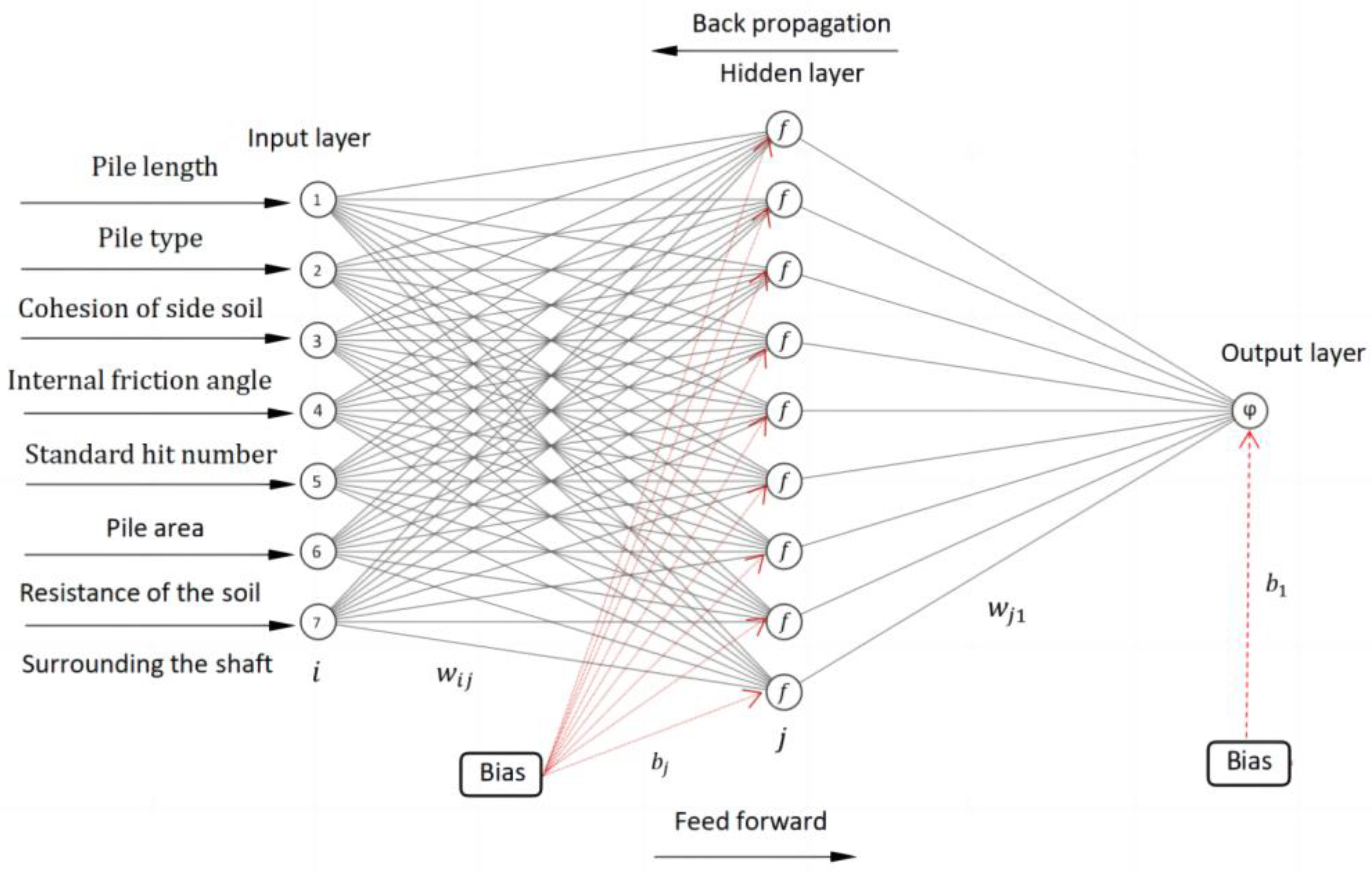
2.1. Predictive Models (ANN, BP)

2.1.1. Artificial Neural Networks

The artificial neural network (ANN) is a powerful and widely used heuristic mathematical calculation model based on physiological research results of the brain that aims to simulate the nervous system and human brain behavior. ANNs have proven to be an effective predictive tool for solving many types of issues in the field of geotechnical engineering, such as retaining wall deflection, excavation, soil properties, site characteristics, pile-bearing capacity, and structural settlement [23]. The mathematician Culloch and neuroscientist Pitts [24] first proposed the concept of an artificial neural network based on the structure of the human brain. They proposed threshold logic units, a group of parallel interconnected processing units, nodes or neurons, which form the basis of ANNs. Each neuron has an activated function, and weights transmit activation signals between nodes. Therefore, the data processing capability of an artificial neural network is closely related to its structure and weights [25].

2.1.2. BP Neural Network

Artificial neural networks use learning algorithms to study the relationship between input and output data through an interactive process. The back-propagation (BP) algorithm is generally considered to be the most popular and effective learning algorithm in multilayer networks [26]. The most basic BP network consists of an input layer, a hidden layer, and an output layer, which is an error back-propagation learning algorithm. Because BP neural networks have the ability to realize arbitrary nonlinear mapping of input and output, a three-layer BP neural network can approximate any nonlinear function with any degree of precision [27]. Although the BP algorithm has shortcomings, such as slow convergence speed and ease of encountering local minima, it is still widely used in pattern recognition, function approximation, and data analysis [28,29]. Since network performance is expected and increasing the number of implied layers too much can lead to a complex model, this study uses only one implied layer to evaluate network performance. The structure of a standard three-layer BP neural network is shown in Figure 1.

2.2. Optimization Models (AGA, APSO)

2.2.1. Genetic Algorithm

The genetic algorithm (GA) is a random search algorithm and optimization technology developed by Holland. It is a widely used and efficient adaptive intelligent algorithm for random global search and optimization [30]. It does not rely on gradient information but searches for the optimal solution by simulating the natural evolution process; one of its main advantages is that it can solve highly nonlinear and complex issues. The GA may serve as a credible solution for most optimization cases, such as geotechnical applications with various loading conditions, linear or nonlinear soil properties, and discontinuous or continuous soil media [31,32]. The flow chart of the BP neural network optimized using the adaptive genetic algorithm in this article is shown in Figure 2.

2.2.2. Particle Swarm Algorithm

The particle swarm optimization (PSO) algorithm was proposed by Kennedy and Everhart and inspired by the social behavior of animals such as fish, insects, and birds [33]. In the PSO algorithm, each candidate can be considered as an “individual in a flock”, and the algorithm simulates a bird in a flock by designing a massless particle with two properties, speed and position, where speed represents the speed of movement and position represents the direction of movement. Each particle searches for the optimal solution independently in the search space, records the solution as the current individual extreme value, and shares the value with other particles in the whole particle swarm so as to find the optimal individual extreme value as the global optimal solution of the entire particle swarm. All particles in the particle swarm adjust their speed and position according to the current individual extreme value found by themselves and the current global optimal solution shared by the entire particle swarm. Because the PSO algorithm does not depend on issue information and uses real numbers to solve, the algorithm has strong versatility, and the parameters do not need much adjustment, which means that the principle is simple and easy to implement. PSO is a powerful population-based algorithm for solving continuous and discretized issues, and it is often used in prediction models of geotechnical engineering [34,35]. In this article, the fusion adaptive particle swarm optimization algorithm was used to optimize the BP model structure, including the threshold and weight, in order to improve the prediction accuracy of the ultimate bearing capacity of the pile foundation. The flow chart of the BP neural network optimized using the adaptive particle swarm optimization algorithm in this article is shown in Figure 3.

3. Modeling Process

3.1. Establishing the Data Set

The 72 sets of data, all located in the Pearl River Delta region, used to calibrate and validate the model were obtained from the literature [36]. For qualitative variables such as the pile type T in the input variable, referring to expert experience and knowledge, the pile types were converted into a distribution number on an integer interval, for example, 1 for precast concrete piles, 2 for immersed cast-in-place piles, 3 for artificial digging piles, and 4 for bored piles. According to Swingler’s suggestion [37], 70% of the data of the whole sample, 52 sets of data, were used to build the training sample set, and the remaining 30% of the data, 20 sets of data, were used to build the test sample set.

Table 1. The applied collected databases [36].

Parameter	Unit	Max	Min	Mean	St.Dv.
L	m	54	6.5	19.89	9.13
A	m2	3.801	0.0707	0.68	0.80
T	-	4	1	2.50	1.12
C	kPa	44	6	24.19	7.86
$\phi$	°	33	5	18.24	6.53
N	-	13.3	4	7.93	2.25
$q_p$	kPa	8100	850	3269.73	1432.97
$Q_u$	kN	19,550	520	4190.14	4468.20

provides information about the databases. The meanings of letters in the table are pile length (L), pile area (A), pile type (T), soil cohesion at pile side (C), internal friction angle ($\phi$), SPT blow count of soil at pile side (N), ultimate end resistance of pile end soil ($q_p$) and actual measured value ($Q_u$), St.Dv. in Table 1 refers to the sample-based estimation standard deviation. In this study, all the algorithms were coded in Matlab2020B software and implemented in the environment of an AMD Ryzen7 5800 H with a Radeon Graphics @3.20 GHz processor and 32.00 GB of installed memory.

3.2. BP Model Establishment

In order to eliminate the influence of dimension, the data were normalized using Formula (1) before the model was established. With the default normalization interval [−1, 1], obviously, there are no negative values for various influencing factors, and here we define their interval as [0, 1]. The normalization formula is as follows:

$$t_{norm}=t_{\min }+\frac{t_{\max }-t_{\min }}{x_{\max }-x_{\min }}(x-x_{\min })$$

(1)

After the completion of the network operation, the data need to be de-normalized to restore them to the order of magnitude of the original data. The restore formula is

$$x_{real}=x_{\min }+\frac{x_{\max }-x_{\min }}{t_{\max }-t_{\min }}(t-t_{\min })$$

(2)

where $t_{norm}$ is the normalized value; $x_{real}$ is the predicted value after being de-normalized; $x_{\mathrm{m}\mathrm{i}\mathrm{n}} \mathrm{a}\mathrm{n}\mathrm{d} x_{\mathrm{m}\mathrm{a}\mathrm{x}}$ are the minimum and maximum values of the variables, respectively; $t_{\mathrm{m}\mathrm{i}\mathrm{n}}$, $t_{\mathrm{m}\mathrm{a}\mathrm{x}}$ are the minimum and maximum values of the normalized variables, respectively.

We used error back-propagation to correct the connection weights and thresholds. Since the output layer knows the ideal output and there is no ideal output for all hidden layers, the correction formulas of the hidden layer and the output layer are different:

$$\begin{array}{c}{w}_{bq}=w_{bq}^{\prime }+\Delta w_{bq}\\ \Delta w_{bq}=a{\delta }_q{o}_b\\ =a{o}_b\left(1-o_q\right)\left(y_q-o_q\right)o_b\end{array}$$

(3)

where ${\omega }_{bq}$ is the connection weight between the $q$-th neuron of the output layer and the $b$-th neuron of its predecessor layer; $o_b$ $\mathrm{a}\mathrm{n}\mathrm{d} o_q$ are actual outputs, $\alpha$ is the learning rate, $0<\alpha <1$.

The hidden layer is calculated as follows:

$$\begin{array}{c}{v}_{cb}=v_{cb}+\Delta v_{cb}\\ \Delta v_{cb}=a{\delta }_{bk-1}{o}_{ck-2}\\ =a{o}_{bk-1}\left(1-o_{bk-1}\right)\left(w_{b1}{\delta }_{1k}+w_{b2}{\delta }_{2k}+\cdots +w_{b{m}_k}{\delta }_{m_{k}k}\right)o_{ck-2}\end{array}$$

(4)

where $v_{cb}$ is the connection weight between the $c$-th neuron of the hidden layer $k-2$ and the $b$-th neuron of the hidden layer $k-1$; $w_{b1},w_{b2},\cdots ,w_{b{m}_k}$ and ${\delta }_{b1},{\delta }_{b2},\cdots ,{\delta }_{b{m}_k}$ are the connection weight and error from the $p$-th neuron in the hidden layer $k-1$ to the $k$ neuron in the hidden layer, respectively, and $\alpha$ is the learning rate, $0<\alpha <1$.

The determination of the number of neurons in the hidden layer is a very important step in the design of the hidden layer, which directly affects the network’s ability to respond to practical engineering issues [28]. The more commonly used hidden layer node calculation formula is as follows (the input node and output node are represented by $m$ and $n$, respectively, and the hidden layer node is represented by $h$):

1.

Kolmogorov theorem [38]:

$$h=2m+1$$

(5)

2.

Empirical formula based on the least squares method [39]:

$$h={\left(0.43mn+2.54m+0.77n+0.35+0.12n^2\right)}^{1/2}+0.51$$

(6)

3.

Golden section method (where a is an integer between 0 and 10):

$$h={\left(m+n\right)}^{1/2}+a$$

(7)

Since all the above methods have the problem of incompatibility, this study adopted the method of trial calculation. According to the above formula, the range of the number of hidden layer neuron nodes is determined as 6–15, and a three-layer BP neural network with an input layer, hidden layer, and output layer is established. The hyperbolic tangent sigmoid function $\left(\mathrm{T}\mathrm{a}\mathrm{n}\mathrm{s}\mathrm{i}\mathrm{g}\right)$ is used between the input layer and the hidden layer, while the linear transfer function $\left(\mathrm{P}\mathrm{u}\mathrm{r}\mathrm{e}\mathrm{l}\mathrm{i}\mathrm{n}\right)$ is used between the hidden layer and the output layer. In order to determine the number of neurons in the hidden layer of the BP algorithm, this article used 52 sets of training data and conducted a large number of simulation experiments with values in the range of 6–15 obtained by the above empirical formula. The mean square error value is shown in Figure 4.

It can be seen from Figure 4 that when the number of neurons in the hidden layer is set to 9, the minimum mean square error of the training sample can be obtained. Therefore, in this article, when there are 7 neurons under the input layer, 9 neurons under the hidden layer, and 1 neuron under the output, the performance of the BP neural network is best. When modeling, the training number is set to 1000; the learning rate is 0.01, the minimum error of the training target is 0.0001, and the maximum number of failures is set to 10. The structure of the BP neural network is shown in Figure 5.

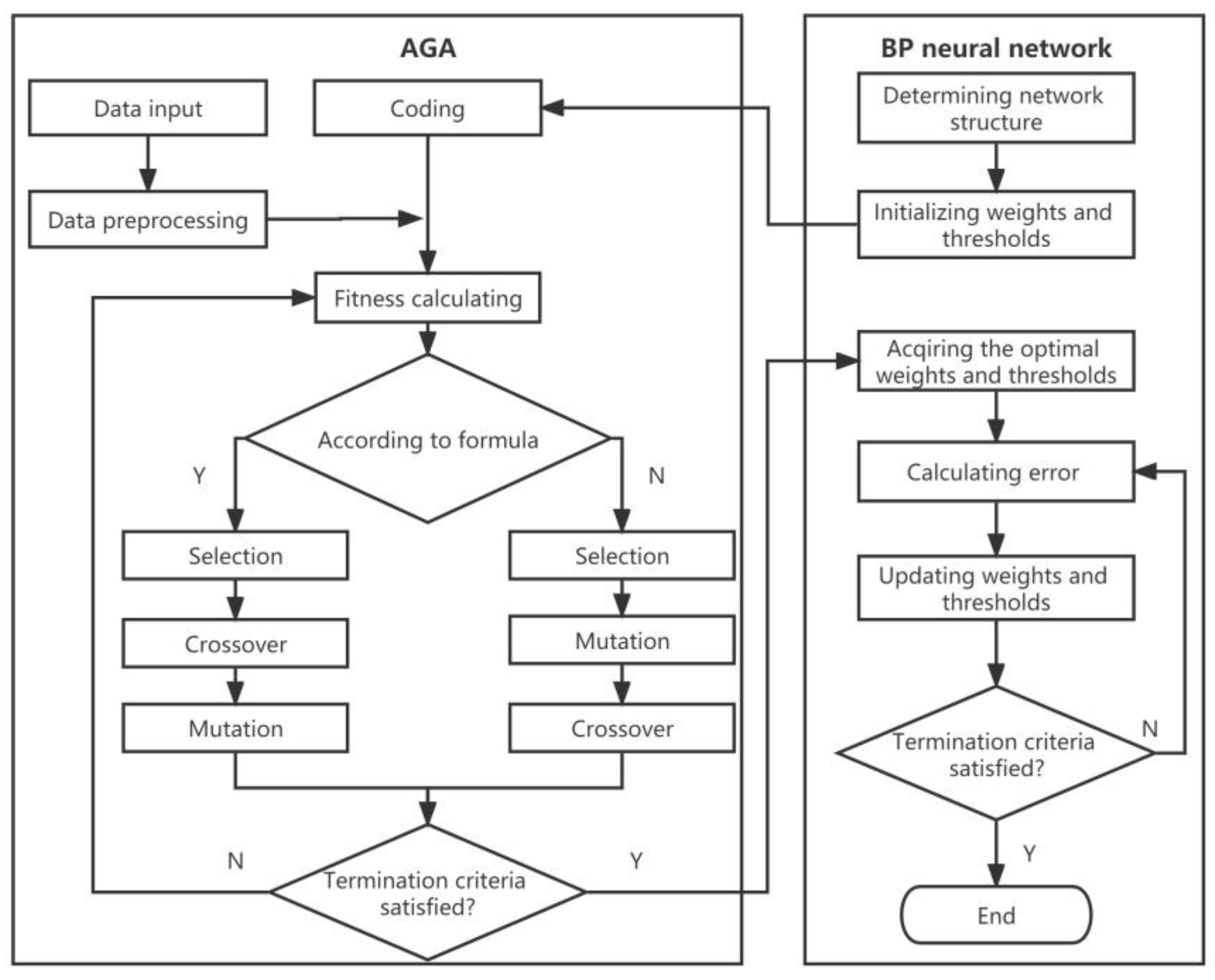
3.3. BP Neural Network Model Based on Adaptive Genetic Algorithm (AGA-BP)

In the process of genetic evolution, individuals in the population need to change the genes carried on the chromosomes through operators such as selection, crossover, and mutation. After each generation of evolution, these superior individuals are selected and can evolve continuously to improve individual fitness. The algorithm tends to converge during a few iterations so that better solutions and individuals may be obtained [40]. However, the convergence, performance, and ability of the GA are seriously affected by the initial population. Based on this situation, Srinivas et al. [41] proposed an adaptive genetic algorithm (AGA) to improve the traditional genetic algorithm. However, when the individual fitness of this algorithm is close to or equal to the maximum fitness, ${\mathrm{P}}_{\mathrm{c}}$ and ${\mathrm{P}}_{\mathrm{m}}$ are close to or equal to zero, which increases the possibility of evolution towards a local optimal solution, which is unfavorable for the initial stage of evolution. Applying Young’s module function in this article, the probability of crossover and mutation was modified by the genetic algorithm. The main idea of this method is that the probability of crossover and mutation increases when the similarity of individual populations tends to be locally optimal and decreases when the fitness of the population is relatively dispersed, which not only improves the search efficiency of the genetic algorithm but also effectively avoids the local minimum problem. The following formula adjusts the crossover rate 1 and variance rate 2:

$$P_c=\{\begin{array}{c}\frac{k_1\left(f_{\max }-f^{\prime }\right)}{f_{\max }-f_{avg}}\\ k_2\end{array}\hspace{1em}\begin{array}{c}{f}^{\prime }\ge f_{avg}\\ f^{\prime }<f_{avg}\end{array}$$

(8)

$$P_m=\{\begin{array}{c}\frac{k_3\left(f_{\max }-f\right)}{f_{\max }-f_{avg}}\\ k_4\end{array}\hspace{1em}\begin{array}{c}f\ge f_{avg}\\ f<f_{avg}\end{array}$$

(9)

It is not difficult to analyze the above two formulas. When the fitness value is just equal to the maximum fitness, the probability of crossover and mutation is almost zero, which means that individuals will no longer cross over and mutate at this time. If this phenomenon occurs at the early stage of evolution, then the selected excellent individuals are not necessarily global optimal, which may cause the algorithm to eventually regress into local optimal. In order to avoid this phenomenon and ensure that the probability of crossover and mutation of individuals with maximum fitness is not zero, this study added two non-zero constants on the basis of the original formula to ensure the smooth progress of the initial stage of the adaptive genetic algorithm. See Equations (10) and (11) for the improved formula.

$$P_c=\{\begin{array}{c}{P}_{c1}-\frac{\left(P_{c1}-P_{c2}\right)\left(f^{\prime }-f_{\max }\right)}{f_{\max }-f_{avg}}\\ P_{c1}\end{array}\hspace{1em}\begin{array}{c}{f}^{\prime }\ge f_{avg}\\ f^{\prime }<f_{avg}\end{array}$$

(10)

$$P_m=\{\begin{array}{c}{P}_{m1}-\frac{\left(P_{m1}-P_{m2}\right)\left(f-f_{\max }\right)}{f_{\max }-f_{avg}}\\ P_{m1}\end{array}\hspace{1em}\begin{array}{c}f\ge f_{avg}\\ f<f_{avg}\end{array}$$

(11)

where $f_{max}$ is the maximum fitness in the group; $f_{avg}$ is the average fitness of each generation; $f^{\prime }$ is the larger fitness value of the two individuals to be crossed; $f$ is the fitness value of the individual to be mutated. In the above formula, the value interval of four non-zero constants, $P_{c1}$ and $P_{c2}$ are generally [0.4, 0.99], $P_{m1}$ and $P_{m2}$ are generally [0.1, 0.001]; in this article $P_{c1}$, $P_{c2}$, $P_{m1}$ and $P_{m2}$ are 0.9, 0.6, 0.1, and 0.01, respectively.

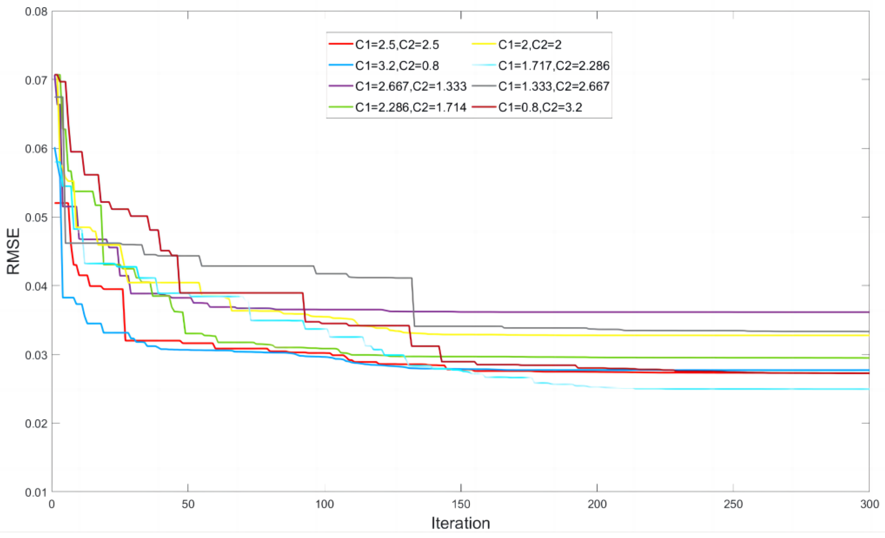
Selection of AGA-BP Parameters

The population size in the genetic algorithm determines the final result of a genetic optimization. If the size of the population is too large, it will lead to too long an optimization time of the genetic algorithm, and if the size of the population is too small, it will easily lead the genetic algorithm to the local optimal solution [21]. Therefore, in this paper, we analyze the optimization accuracy and the optimization time of the algorithm under different population sizes. The calculation results are shown in

Table 2. Accuracy and simulation time of the optimization algorithm for different total cluster sizes.

Population Size	Average Absolute Error	Minimum Error Value	Simulation Time (Second)
10	0.038142	0.021556	15.62
20	0.025484	0.0033629	41.33
30	0.009778	0.0057508	44.14
40	0.023702	0.0052848	82.40
50	0.019769	0.0049129	92.69
60	0.016872	0.0058662	116.76
70	0.010416	0.0020544	203.29
80	0.016348	0.0035507	276.18
90	0.013775	0.0049619	301.90
100	0.18456	0.0024573	328.65

.

Comparing the error accuracy and simulation time required shown in Table 2, this paper chooses 70 as the population size so that the simulation accuracy and simulation time are moderate. When the population size is determined, the default number of iterations is set to 150, and according to the results of several runs, the algorithm stops running when it basically reaches the optimal value at about 100 iterations. Therefore, in this paper, the number of iterations of the genetic algorithm is set to 120 by slightly increasing the number of iterations based on 100.

The process of creating the network model is as follows:

• Use the basic principle of the BP neural network to establish the topology structure of the BP neural network according to the input and output sample sets;
• Form an initialization population;
• Calculate the fitness value of all individuals in the population.
• Perform the genetic operations of selection, crossover, and mutation in turn, adaptively adjust the crossover and mutation rate in the evolution process, select excellent individuals as the parent generation, and then reproduce the next generation;
• Determine whether the termination condition of genetic evolution has been reached. If the condition is met, go to the next step, otherwise go to step 3;
• Obtain the optimal solution, extract the solution with the highest fitness, and assign the value to the BP neural network for training and learning.

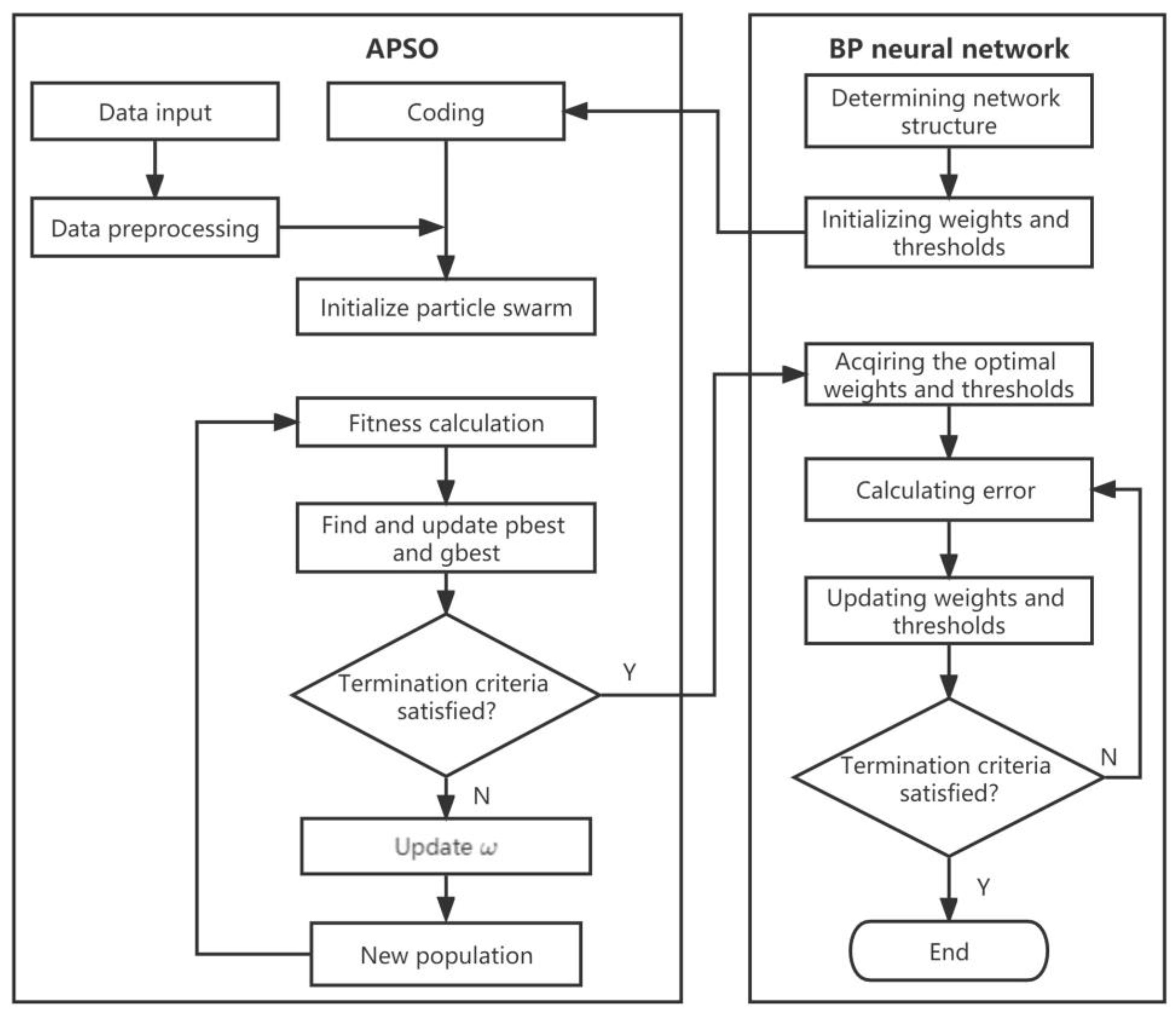
3.4. BP Neural Network Model Fusion Adaptive Particle Swarm (APSO-BP)

Particle swarm optimization, used widely in search algorithms, is an intelligent algorithm based on swarm optimization in which each individual or each potential candidate is described as a “particle” [42]. In this study, real number coding was used to initialize the position vector of the individual population, which means the position vector of each particle corresponds to a set of connection weights and thresholds of the BP neural network.

In the particle swarm optimization algorithm, it is assumed that there is an n-dimensional target search space. Each particle is regarded as a point in space, and N particles constitute a group. Each particle consists of a vector $x_i=\left(x_{i1},x_{i2},\cdots ,x_{id}\right)$ which indicates the position; another vector $v_i=\left(v_{i1},v_{i2},\cdots ,v_{id}\right)$ indicates speed; during training and learning, particle velocity and position are adjusted by the following formulas:

$$v_i^{k+1}=\omega v_i^k+c_1\times r_1\times (P_i-x_i^k)+c_2\times r_2\times (P_g-x_i^k)$$

(12)

$$x_i^{k+1}=x_i^k+v_i^{k+1},\hspace{1em}i=\mathrm{1,2},\cdots ,n$$

(13)

where $i$ is the $i\mathrm{th}$ particle in the population; $c_1$, $c_2$ represent non-social cognitive coefficients; $r_1$, $r_2$ are two random numbers distributed in the range of [0, 1]; $\omega$ is the inertia weight; the vector $P_i=(P_{i1},P_{i2},y,P_{iN})$ is the best fitness position of particle $i,\mathrm{c}\mathrm{a}\mathrm{l}\mathrm{l}\mathrm{e}\mathrm{d} pbest;\mathrm{t}\mathrm{h}\mathrm{e} \mathrm{v}\mathrm{e}\mathrm{c}\mathrm{t}\mathrm{o}\mathrm{r}$ $P_g=(P_{g1},P_{g2},y,P_{gN})$ is the best particle among all the particles in the position group of particle $i$ called $gbest$: the value of each component in $v_i$ should be limited to the range of $\left[-v_{max},v_{max}\right]$ to prevent each particle from over-roaming outside the search space.

Since the inertia weight $\omega$ with a constant value cannot perform an accurate local search in the later stage of calculation, this article uses the linear decreasing dynamic inertia weight to guide the algorithm from global search to local search through its own changes so as to ensure the stability of the algorithm in the later operation. The calculation formula is as follows:

$$\omega ={\omega }_{max}-\left({\omega }_{max}-{\omega }_{min}\right){\left(\frac{k}{T_{max}}\right)}^2$$

(14)

where ${\omega }_{max} \mathrm{a}\mathrm{n}\mathrm{d} {\omega }_{min}$ are the maximum and minimum values of the inertia weight, respectively; $T_{max}$ represents the maximum number of iterations, and $k$ represents the current number of iterations.

Selection of APSO-BP Parameters

For the first stage of model design, there is a need to obtain the optimal population size considering a parametric analysis. Regarding that, values of 25, 50, 75, 100, 150, 200, 250, and 300 were used to determine the size of the population in the network model, and the results of parametric research are shown in

Table 3. Results of APSO-BP models with different swarm size values.

Model No.	Swarm Size	APSO-BP Results				Ranking				Total Score	Total Ranking
		Training		Testing		Training		Testing
		RMSE	R2	RMSE	R2	RMSE	R2	RMSE	R2
1	25	0.0362	0.9769	0.0446	0.9709	4	4	1	1	10	7
2	50	0.0366	0.9766	0.0407	0.9759	3	3	2	2	10	7
3	75	0.0317	0.9823	0.0304	0.9865	6	6	8	8	28	1
4	100	0.0401	0.9717	0.0337	0.9838	1	1	6	6	14	6
5	150	0.0272	0.9865	0.0378	0.9791	8	7	3	3	21	3
6	200	0.0328	0.9810	0.0368	0.9795	5	5	4	4	18	4
7	250	0.0281	0.9872	0.0364	0.9818	7	8	5	5	25	2
8	300	0.0371	0.9765	0.0326	0.9849	2	2	7	7	18	4

. Other effective parameters of APSO were considered constant when this research was conducted (C1 = C2 = 2; the maximum number of iterations is 100; $\omega$ is automatically adjusted by Equation (14)). The ranking system used in Table 3 is based on the method studied by Zorlu et al. [43]. According to this method, each performance metric (i.e., root mean square error RMSE and coefficient of determination R² here) is ranked in its category. For example, the smallest value in RMSE for the trained model receives the highest score, and the smallest value in R² receives the largest score. Therefore, an overall ranking score of 28 was the best model, and 75 was chosen as the best population size.

Table 4. The applied collected databases [36].

No.	L (m)	A (m2)	T	C (kPa)	$\mathit{\phi }$ (°)	N	${\mathit{q}}_{\mathit{p}}$ (kPa)	${\mathit{Q}}_{\mathit{u}}$ (kN)
1	24.24	0.1963	1	28	21.2	9.2	3400	3190
2	28.8	0.1590	1	13	21.0	8.5	4000	2860
3	13.64	0.0908	2	31	20.5	8.3	1600	600
4	16.57	0.2827	2	37	15.4	7.4	4200	2000
5	24.68	3.8013	3	23	10.5	6.3	3600	16,800
6	14.2	0.7854	3	34	18.5	7.9	3800	2160
7	14.63	0.1257	1	24	16.7	7.2	2100	630
8	12.32	0.2827	4	25	18.1	6.9	1200	1100
9	11.53	1.5394	3	25	20.0	7.1	6500	12,000
10	33.22	0.7854	4	19	22.0	8.4	2400	5650
11	8.55	0.2827	4	23	30.5	13.1	850	660
12	22.19	0.1810	2	42	22.6	7.8	3000	1700
13	6.78	0.1257	4	34	15.4	4.7	1300	520
14	27.86	0.7854	4	22	14.4	6.5	2800	5760
15	27.95	0.1963	2	41	11.3	5.6	5000	3000
16	20.95	1.7671	3	18	5.0	4.0	5000	10,160
17	18.47	0.1590	1	28	6.6	5.3	5100	2500
18	21.55	0.1257	1	15	22.1	9.7	4300	1800
19	18.35	1.1310	3	30	22.4	8.7	4700	7380
20	24.12	0.3318	2	34	10.2	6.0	3900	3450

presents the 20 sets of data used for testing.

As shown in Figure 6, we conducted sensitivity analysis through eight groups of values, the $c_1$ and $c_2$ in the figure are the learning factors of the algorithm. When the total group size was 75, and the evolutionary algebra was 300, the optimal combination of coefficients $c_1$ and $c_2$ was obtained for predicting the ultimate bearing capacity of the pile foundation. At this time, $c_1$ is 1.714 and $c_1$ is 2.286. In this algorithm, the maximum value of the adaptive inertia weight ${\omega }_{max}$ is 0.9; the minimum value ${\omega }_{min}$ is 0.4; the maximum number of iterations $T_{max}$ is 60; the number of termination iterations of the BP algorithm in the final stage is 10; the learning rate $\alpha$ is 0.01; and the minimum error of the training target $\epsilon$ is $E^{-6}$.

This article sets an evolutionary strategy selection probability for the defects of the BP neural network: $T_t=k/T_{max}$, namely $T_r$ changes from $1/T_{max}$ to 1 as the number of iterations increases. When the random number $r<T_r$, the error back-propagation is used to correct the connection weight and threshold. After the correction is completed, it is re-encoded to form a new particle position, and this position is directly used to compare and update the global optimal position. Otherwise, Equations (12)–(14) are used to update the current individual. The algorithm can be summarized in the following steps:

• Use the basic principle of the BP neural network, according to the input and output sample sets, to establish the topology structure of the BP neural network;
• Calculate the fitness value of the particle;
• Update the individual optimal position pbest and the global optimal position gbest;
• Update the current population through the particle learning strategy of the hybrid BP neural network;
• Run until termination criteria are met, the connection weight and threshold corresponding to the global optimal position are output to the BP neural network; otherwise, return to the second step;
• Continue training with the optimized BP neural network until the termination condition is met, and output the trained network.

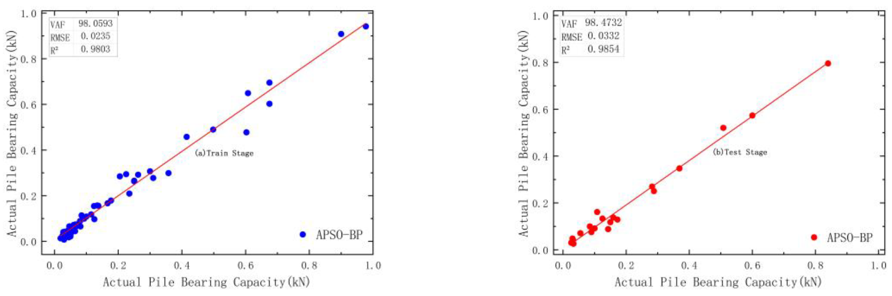
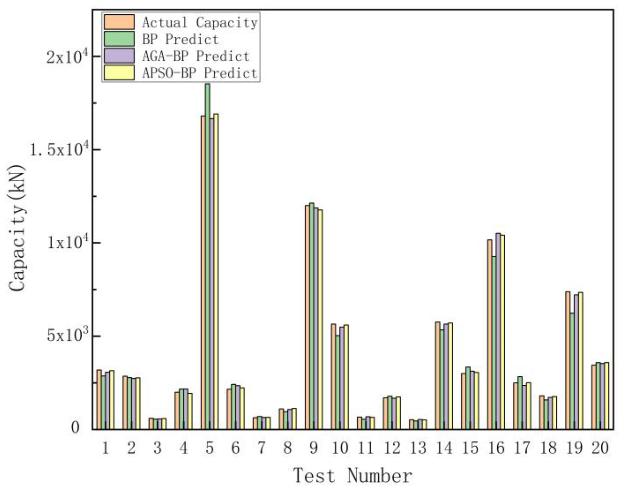
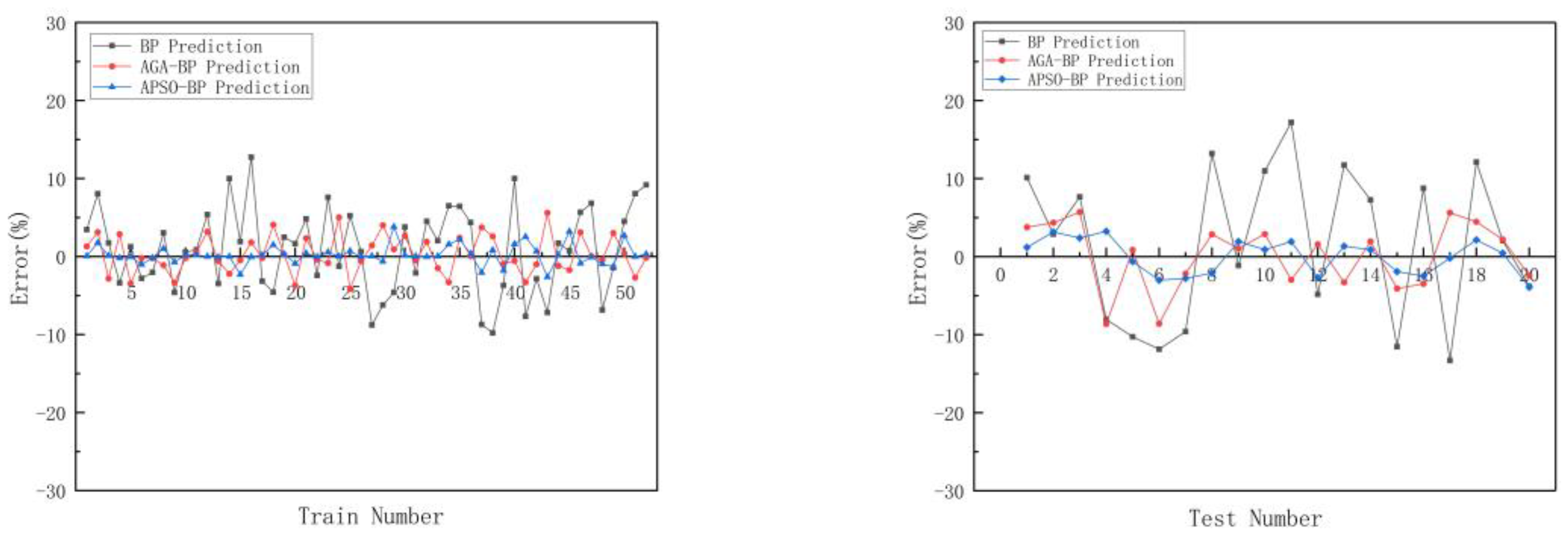
4. Model Prediction Results and Discussion

This research used three machine learning algorithms, namely, the back-propagation neural network, adaptive genetic algorithm-optimized BP network, and fusion adaptive particle swarm optimization-optimized BP network, to construct a prediction model in order to verify the best fitting model for predicting the ultimate bearing capacity of pile foundations. The prediction performance of the developed prediction model was evaluated by calculating the coefficient of determination (R²), value account for (VAF), and the root mean square error (RMSE):

$$R^2=1-\frac{{{\sum }_{i=1}^n\left(y-y^{\prime }\right)}^2}{{{\sum }_{i=1}^n\left(y-\overline{y}\right)}^2}i=1,2,3,\cdots ,n$$

(15)

$$VAF=\left[1-\frac{\mathit{var}\left(y-y^{\prime }\right)}{\mathit{var}\left(y\right)}\right]\times 100$$

(16)

$$RMSE=\sqrt{\frac{1}{n}{\sum }_{i=1}^n{\left(y-y^{\prime }\right)}^2}\hspace{1em}i=\mathrm{1,2},3,\cdots ,n$$

(17)

In the above formulas, $y$ is the measured value; $y^{\prime }$ is the predicted value; $\overline{y}$ is the average value; $n$ is the total number of samples. Theoretically, when the performance results of the prediction model are $R^2=1$, $RMSE=0$ and $VAF=100\%$, the prediction model is optimal.

For comparison,

Table 5. Performance comparison for the proposed predictive models.

Model	System Results						Ranking						Total Score	Total Ranking
	Train			Test			Train			Test
	R2	VAF	RMSE	R2	VAF	RMSE	R2	VAF	RMSE	R2	VAF	RMSE
BP-ANN	0.9136	90.2796	0.0889	0.9085	91.9316	0.0938	1	3	1	1	3	1	10	3
AGA-BP	0.9702	97.0672	0.0494	0.9772	97.8348	0.0436	2	2	2	2	2	2	12	2
APSO-BP	0.9803	98.0593	0.0387	0.9854	98.4732	0.0332	3	1	3	3	1	3	14	1

lists the performance index calculation results of the best BP, AGA-BP, and APSO-BP models used in the data training and testing stage. The training results of the AGA-BP model and APSO-BP model were 0.9702, 97.0672, 0.0494, and 0.9803, 98.0593, 0.0387, respectively, and the test results were 0.9772, 97.8348, 0.0436 and 0.9854, 98.4732, 0.0332. Since the best results of the two models are very close, the simple ranking method was also used to score different parts of the evaluation results of the three machine learning algorithms. Using the allocation method described above, the score allocation rules are as follows: the model with the lowest systematic error RMSE will receive the largest score, the highest R² will receive the largest score, and the highest VAF will receive the lowest score. These scores were used for the testing and training parts of the model. Finally, based on the scores of each part of the model, the model with the highest score was determined as the optimal model (see the last column of Table 5).

According to Table 5, the total scores of the BP-ANN, AGA-BP, and APSO-BP models in ${\mathrm{Q}}_{\mathrm{u}}$ prediction are 10, 12, and 14 points, respectively. According to the score results, the APSO-BP model has the best predictive effect. The relationships between the three best models for predicting the ultimate bearing capacity of piles tested and the measured model on the training data set are shown in Figure 7, Figure 8 and Figure 9.

As can be seen from Figure 8, Figure 9 and Figure 10, the VAF, RMSE, and R² of the BP-ANN test sets are 91.9316, 0.0938, and 0.9085, respectively; the VAF, RMSE, and R² of the AGA-BP test sets are 97.8348, 0.0436 and 0.9772, respectively; the sets of the APSO-BAP test were 98.4732, 0.0332, and 0.9854, respectively. The R² values in the figures are all above 0.9, indicating that the measured value of the bearing capacity of the training data set is consistent with the predicted value. The coefficient of determination between the predicted bearing capacity of the pile foundation and its measured bearing capacity in Figure 8 and Figure 9 is above 0.97, indicating that the two optimization models established in this article are effective. In addition, for comparison with other machine learning methods, this study compared the training and test sets obtained by some prediction methods in the references with the two models established and carried out a score ranking. The specific data are shown in

Table 6. Performance comparison for the proposed predictive models with others.

Models	Training Data Set		Testing Data Set		Ranking				Total Score	Total Ranking
	R2	RMSE	R2	RMSE	Train		Test
ANN [21]	0.809	0.116	0.99	0.108	1	2	1	2	6	9
GP [11]	0.976	0.051	0.986	0.040	9	6	9	7	31	2
GA-ANN [21]	0.96	0.1072	0.99	0.0447	4	3	5	5	17	8
FP-GMDH [13]	0.97	0.0594	0.96	0.0647	7	5	7	4	23	6
ANFIS-GMDH-GSA [13]	0.965	0.065	0.94	0.082	6	4	6	3	19	7
LMR [44]	0.835	1.737	0.751	1.767	2	1	2	1	6	9
GA-SVR [18]	0.955	0.051	0.943	0.031	5	6	4	9	24	5
TLBO-ANN [25]	0.941	0.035	0.943	0.030	3	10	3	10	26	4
AGA-BP	0.9702	0.0494	0.9772	0.0436	8	8	8	6	30	3
APSO-BP	0.9803	0.0387	0.9854	0.0332	10	9	10	8	37	1

.

Table 6 compares the training and testing values obtained by different methods for predicting the ultimate bearing capacity of the pile foundation in eight references with the two optimization methods in this article. According to the results, the top three are the GP model, AGA-BP model, and APSO-BP model, with scores of 31 points, 30 points, and 37 points, respectively. The determination coefficients of the predicted values and measured values obtained by the three methods are higher, and the fitting effect is better. The predicted results are more accurate, and the APSO-BP model has the highest score among the three methods, which shows that the optimization model proposed in this article has good predicted results.

Figure 10 shows the comparison results between test data and real data for all models. Compared with the predicted results of the BP-ANN, the yellow and purple lines in the figure fit the expected lines better, indicating that both the proposed AGA-BP model and the proposed APSO-BP model can be used to predict the ultimate bearing capacity of piles and the predicted results of the BP network model optimized by the adaptive particle swarm algorithm are more accurate.

Figure 11 shows the relative error percentage of training samples and test samples. From the training set, the maximum prediction error of the BP model is 12%, and the minimum is 0.6%; the maximum prediction error of the AGA-BP model is 5.6%, and the minimum prediction error is 0.1%; the maximum prediction error of APSO-BP model is 3.8%, and the minimum prediction error is 0.05%. From the test set, the maximum prediction error of the BP model is 17%, and the minimum is 1.1%; the maximum prediction error of the AGA-BP model is 8.5%, and the minimum prediction error is 0.8%; the maximum prediction error of the APSO-BP model is 3.9%, and the minimum prediction error is 0.2%. Overall, the prediction results of the BP model fluctuate greatly, and the accuracy of the AGA-BP model prediction results compared to the BP model prediction results significantly indicates that the prediction results of the APSO-BP model are closest to the measured values. This indicates that the model has high accuracy and can provide a new method for predicting the ultimate bearing capacity of pile foundations.

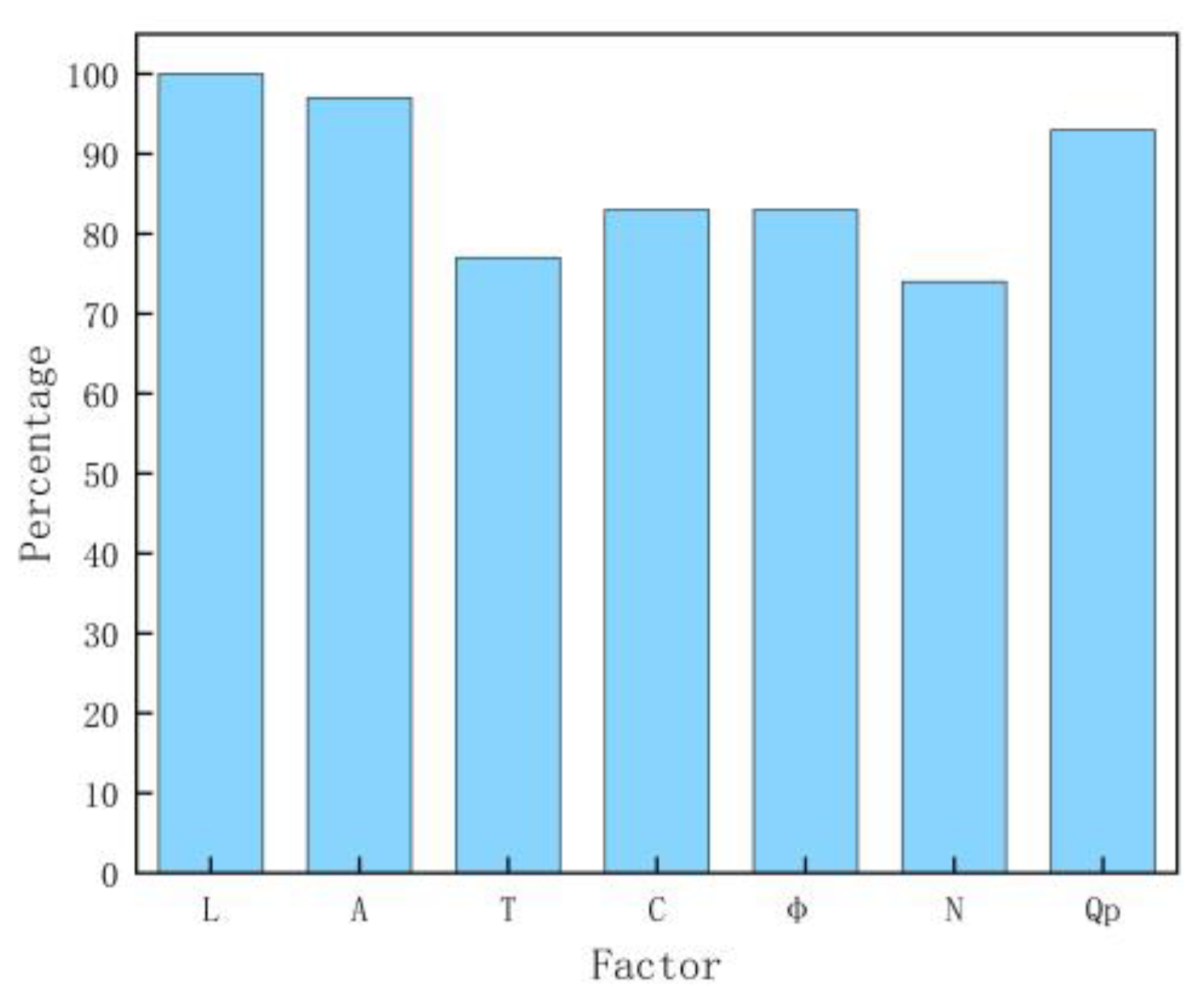
5. Sensitivity Analysis

In order to evaluate the importance of the selected independent variables in predicting the ultimate load capacity of the pile foundations, a sensitivity analysis was carried out in this paper by examining all the input factors affecting the pile Q_u. To achieve this, Yong et al. [45]. mentioned that after obtaining the optimal structure of the network, this structure was run 30 times with the collected data set to see how many parameters were designed after each run. For example, in this study, the sensitivity analysis for parameter L was 100%, meaning that this parameter appeared in the best procedure for each BP network evolution and had the greatest impact on the results of the network runs. The sensitivity analysis for parameter C was 83%, meaning that this parameter appeared in 25 of the 30 best procedures for BP network evolution ($\frac{25\times 100}{30}=83\%$). Figure 12 illustrates the frequency of occurrence of the input factors for this study; as far as the results are concerned, the ultimate bearing capacity of the pile is more influenced by L (pile length), A (area of the pile), and Q_p (ultimate resistance of the soil at the end of the pile). The results obtained from this analysis are in accordance with the conventional logic of pile–soil interaction.

6. Summary and Conclusions

In this study, two optimized neural network models were established to predict the ultimate bearing capacity of a pile foundation. The following conclusions can be drawn through the predicted results and comparative analysis:

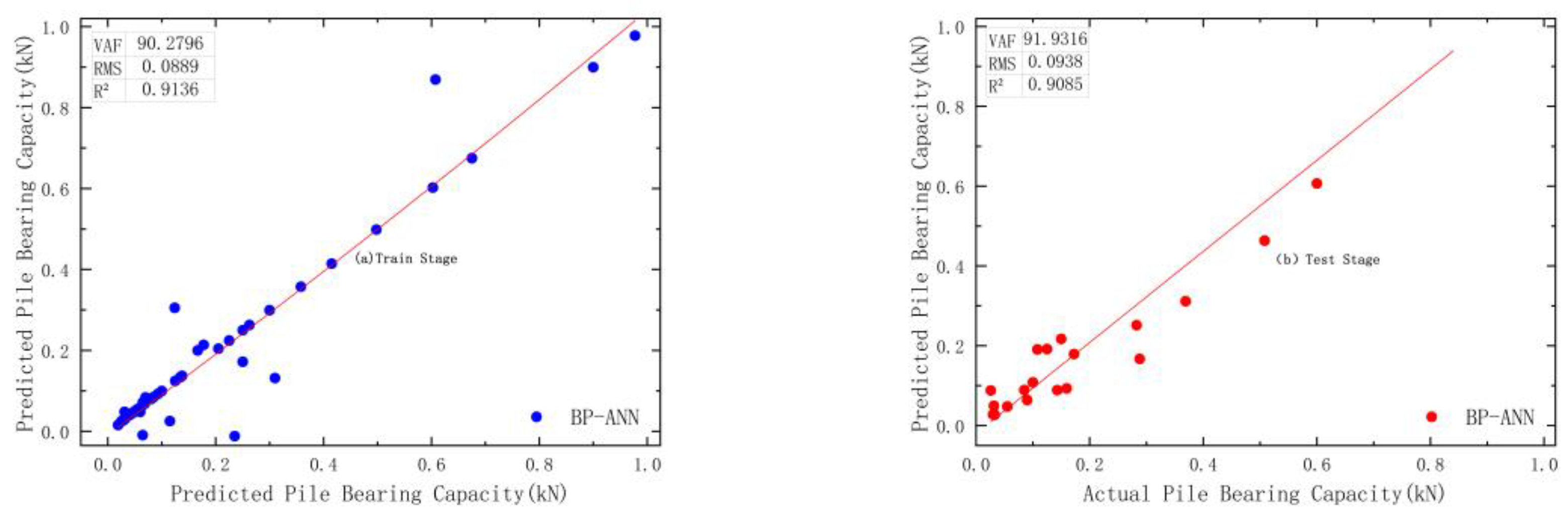
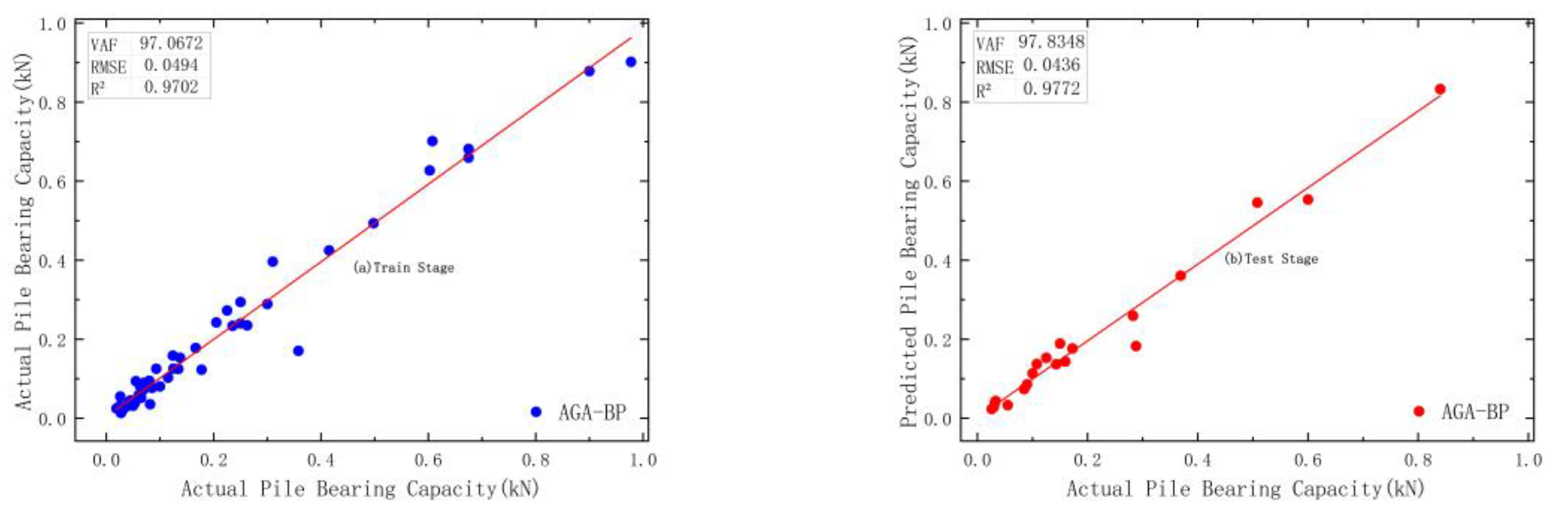
• For the prediction of the ultimate bearing capacity of the pile foundation, one BP neural network and two optimization network models are constructed. The prediction results are in good agreement with the measured data, and the correlation coefficients R² of the test results are 0.9085, 0.9772, and 0.9854. When it is impossible to conduct a load test on each pile foundation in the construction of the project, the model can be used to predict the bearing capacity based on a small amount of test data, and the results can be used as a reference for design and shorten the project cycle.
• According to the performance of the model in the test set, R², VAF, and RMSE were used to comprehensively evaluate the model. According to the comparison results, the BP neural network optimized by the adaptive particle swarm optimization algorithm had high accuracy, with an absolute error percentage of 2%. The predicted results of this model can provide a certain guiding significance and reference value for the design and calculation of pile foundation engineering.
• The performance of the proposed network model was compared with the results of the ANN, GP, and LMR models in the literature for predicting the ultimate bearing capacity of pile foundations. Through a comprehensive ranking of the training and test sets, the APSO-BP model proposed in this paper ranked first with a final score of 37. Based on the reference comparison with this method, we can see that the proposed neural network model outperforms other prediction methods and can achieve high accuracy in predicting the ultimate bearing capacity of pile foundations.
• With the accumulation of pile-bearing capacity test data, the developed APSO-BP model will be further optimized and attain higher prediction accuracy.

References

1. Kordjazi, A.; Nejad, F.P.; Jaksa, M.B. Prediction of ultimate axial load-carrying capacity of piles using a support vector machine based on CPT data. Comput. Geotech. 2014, 55, 91–102. [Google Scholar] [CrossRef]
2. Heins, E.; Grabe, J. FE-based identification of pile–soil interactions from dynamic load tests to predict the axial bearing capacity. Acta Geotech. 2019, 14, 1821–1841. [Google Scholar] [CrossRef]
3. Shooshpasha, I.; Hasanzadeh, A.; Taghavi, A. Prediction of the axial bearing capacity of piles by SPT-based and numerical design methods. Int. J. GEOMATE 2013, 4, 560–564. [Google Scholar] [CrossRef]
4. Hasanzadeh, A.; Shooshpasha, I. Numerical determination of the end bearing capacity of drilled shafts in sand. Jordan J. Civ. Eng. JJCE 2017, 11, 501–511. [Google Scholar]
5. Qi, C.-G.; Liu, G.-B.; Wang, Y.; Deng, Y.-B. A design method for plastic tube cast-in-place concrete pile considering cavity contraction and its validation. Comput. Geotech. 2015, 69, 262–271. [Google Scholar] [CrossRef]
6. Sakr, M. Comparison between high strain dynamic and static load tests of helical piles in cohesive soils. Soil Dyn. Earthq. Eng. 2013, 54, 20–30. [Google Scholar] [CrossRef]
7. Amjad, M.; Ahmad, I.; Ahmad, M.; Wróblewski, P.; Kamiński, P.; Amjad, U. Prediction of Pile Bearing Capacity Using XGBoost Algorithm: Modeling and Performance Evaluation. Appl. Sci. 2022, 12, 2126. [Google Scholar] [CrossRef]
8. Moayedi, H.; Hayati, S. Artificial intelligence design charts for predicting friction capacity of driven pile in clay. Neural Comput. Appl. 2019, 31, 7429–7445. [Google Scholar] [CrossRef]
9. Borthakur, N.; Dey, A.K. Evaluation of Group Capacity of Micropile in Soft Clayey Soil from Experimental Analysis Using SVM-Based Prediction Model. Int. J. Geomech. 2020, 20, 04020008.1–04020008.17. [Google Scholar] [CrossRef]
10. Pham, T.A.; Ly, H.-B.; Tran, V.Q.; Giap, L.V.; Vu, H.-L.T.; Duong, H.-A.T. Prediction of Pile Axial Bearing Capacity Using Artificial Neural Network and Random Forest. Appl. Sci. 2020, 10, 1871. [Google Scholar] [CrossRef]
11. Chen, W.; Sarir, P.; Bui, X.; Nguyen, H.; Tahir, M.; Armaghani, D.J. Neuro-genetic, neuro-imperialism and genetic programing models in predicting ultimate bearing capacity of pile. Eng. Comput. 2020, 36, 1101–1115. [Google Scholar] [CrossRef]
12. Dehghanbanadaki, A.; Khari, M.; Amiri, S.; Armaghani, D.J. Estimation of ultimate bearing capacity of driven piles in c-φ soil using mlp-gwo and anfis-gwo models: A comparative study. Soft Comput. 2021, 25, 4103–4119. [Google Scholar] [CrossRef]
13. Harandizadeh, H.; Toufigh, M.M.; Toufigh, V. Application of improved ANFIS approaches to estimate bearing capacity of piles. Soft Comput. 2018, 23, 9537–9549. [Google Scholar] [CrossRef]
14. Bagińska, M.; Srokosz, P.E. The Optimal ANN Model for Predicting Bearing Capacity of Shallow Foundations trained on Scarce Data. KSCE J. Civ. Eng. 2018, 23, 130–137. [Google Scholar] [CrossRef]
15. Karimipour, A.; Abad, J.M.N.; Fasihihour, N. Predicting the load-carrying capacity of GFRP-reinforced concrete columns using ANN and evolutionary strategy. Compos. Struct. 2021, 275, 114470. [Google Scholar] [CrossRef]
16. AlzoUbi, A.K.; Ibrahim, F. Predicting the pile static load test using backpropagation neural network and generalized regression neural network—A comparative study. Int. J. Geotech. Eng. 2018, 15, 810–821. [Google Scholar] [CrossRef]
17. Panda, S.; Panda, G. Fast and improved backpropagation learning of multi-layer artificial neural network using adaptive activation function. Expert Syst. 2020, 37, e12555. [Google Scholar] [CrossRef]
18. Luo, Z.; Hasanipanah, M.; Amnieh, H.B.; Brindhadevi, K.; Tahir, M.M. GA-SVR: A novel hybrid data-driven model to simulate vertical load capacity of driven piles. Eng. Comput. 2019, 37, 823–831. [Google Scholar] [CrossRef]
19. Zhang, T.; Li, X. The Backpropagation Artificial Neural Network Based on Elite Particle Swam Optimization Algorithm for Stochastic Linear Bilevel Programming Problem. Math. Probl. Eng. 2018, 2018, 1626182. [Google Scholar] [CrossRef]
20. Saffaran, A.; Moghaddam, M.A.; Kolahan, F. Optimization of backpropagation neural network-based models in EDM process using particle swarm optimization and simulated annealing algorithms. J. Braz. Soc. Mech. Sci. Eng. 2020, 42, 73. [Google Scholar] [CrossRef]
21. Momeni, E.; Nazir, R.; Armaghani, D.J.; Maizir, H. Prediction of pile bearing capacity using a hybrid genetic algorithm-based ANN. Measurement 2014, 57, 122–131. [Google Scholar] [CrossRef]
22. Singh, G.; Walia, B.S. Performance evaluation of nature-inspired algorithms for the design of bored pile foundation by artificial neural networks. Neural Comput. Appl. 2016, 28, 289–298. [Google Scholar] [CrossRef]
23. Moayedi, H.; Mosallanezhad, M.; Rashid, A.S.A.; Jusoh, W.A.W.; Muazu, M.A. A systematic review and meta-analysis of artificial neural network application in geotechnical engineering: Theory and applications. Neural Comput. Appl. 2019, 32, 495–518. [Google Scholar] [CrossRef]
24. Culloch, W.; Pitts, W.H. A logical calculus of the ideas immanent in neural nets. Bull. Math. Biophys. 1943, 5, 115–133. [Google Scholar] [CrossRef]
25. Benali, A.; Hachama, M.; Bounif, A.; Nechnech, A.; Karray, M. A TLBO-optimized artificial neural network for modeling axial capacity of pile foundations. Eng. Comput. 2019, 37, 675–684. [Google Scholar] [CrossRef]
26. Chen, Y.; Zhang, J.; Liu, Y.; Zhao, S.; Zhou, S.; Chen, J. Research on the Prediction Method of Ultimate Bearing Capacity of PBL Based on IAGA-BPNN Algorithm. IEEE Access 2020, 8, 179141–179155. [Google Scholar] [CrossRef]
27. Luo, J.; Ren, R.; Guo, K. The deformation monitoring of foundation pit by back propagation neural network and genetic algorithm and its application in geotechnical engineering. PLoS ONE 2020, 15, e0233398. [Google Scholar] [CrossRef]
28. Hua, H.; Xie, X.; Sun, J.; Qin, G.; Tang, C.; Zhang, Z.; Ding, Z.; Yue, W. Graphene Foam Chemical Sensor System Based on Principal Component Analysis and Backpropagation Neural Network. Adv. Condens. Matter Phys. 2018, 2018, 2361571. [Google Scholar] [CrossRef]
29. Hughes, T.W.; Minkov, M.; Shi, Y.; Fan, S. Training of photonic neural networks through in situ backpropagation and gradient measurement. Optica 2018, 5, 864–871. [Google Scholar] [CrossRef]
30. Holland, J.H. Adaptation in Natural and Artificial Systems; MIT Press: Cambridge, MA, USA, 1975. [Google Scholar]
31. Moayedi, H.; Raftari, M.; Sharifi, A.; Jusoh, W.A.W.; Rashid, A.S.A. Optimization of ANFIS with GA and PSO estimating α ratio in driven piles. Eng. Comput. 2019, 36, 227–238. [Google Scholar] [CrossRef]
32. Moayedi, H.; Moatamediyan, A.; Nguyen, H.; Bui, X.-N.; Bui, D.T.; Rashid, A.S.A. Prediction of ultimate bearing capacity through various novel evolutionary and neural network models. Eng. Comput. 2019, 36, 671–687. [Google Scholar] [CrossRef]
33. Eberhart, R.; Kennedy, J. A new optimizer using particle swarm theory. In Proceedings of the Mhs95 Sixth International Symposium on Micro Machine & Human Science, Nagoya, Japan, 4–6 October 1995. [Google Scholar]
34. Zhao, W.; Wang, L.; Zhang, Z. A novel atom search optimization for dispersion coefficient estimation in groundwater. Future Gener. Comput. Syst. 2019, 91, 601–610. [Google Scholar] [CrossRef]
35. Harandizadeh, H.; Armaghani, D.J.; Khari, M. A new development of ANFIS–GMDH optimized by PSO to predict pile bearing capacity based on experimental datasets. Eng. Comput. 2019, 37, 685–700. [Google Scholar] [CrossRef]
36. Liu, Y.J. Study of prediction method of vertical ultimate bearing capacity of single pile based on genetic algorithm and neural network. Rock Soil Mech. 2004, 25, 59–63. [Google Scholar]
37. Swingler, K. Applying Neural Networks—A Practical Guide; Academic Press: Cambridge, MA, USA, 1996. [Google Scholar]
38. Krková, V. Kolmogorov’s theorem and multilayer neural networks. Neural Netw. 1992, 5, 501–506. [Google Scholar] [CrossRef]
39. Mitra, M.; Samanta, R.K. Cardiac Arrhythmia Classification Using Neural Networks with Selected Features. Procedia Technol. 2013, 10, 76–84. [Google Scholar] [CrossRef]
40. Pham, T.A.; Tran, V.Q.; Vu, H.T.; Ly, H.B. Design deep neural network architecture using a genetic algorithm for estimation of pile bearing capacity. PLoS ONE 2020, 15, e0243030. [Google Scholar] [CrossRef]
41. Srinivas, M.; Patnaik, L.M. Adaptive probabilities of crossover and mutation in genetic algorithms. IEEE Trans. Syst. Man Cybern. 2002, 24, 656–667. [Google Scholar] [CrossRef]
42. Wang, B.; Moayedi, H.; Nguyen, H.; Foong, L.K.; Rashid, A.S.A. Feasibility of a novel predictive technique based on artificial neural network optimized with particle swarm optimization estimating pullout bearing capacity of helical piles. Eng. Comput. 2020, 36, 1315–1324. [Google Scholar] [CrossRef]
43. Zorlu, K.; Gokceoglu, C.; Ocakoglu, F.; Nefeslioglu, H.A.; Acikalin, S. Prediction of uniaxial compressive strength of sandstones using petrography-based models. Eng. Geol. 2008, 96, 141–158. [Google Scholar] [CrossRef]
44. Armaghani, D.J.; Faradonbeh, R.S.; Rezaei, H.; Rashid, A.S.A.; Amnieh, H.B. Settlement prediction of the rock-socketed piles through a new technique based on gene expression programming. Neural Comput. Appl. 2016, 29, 1115–1125. [Google Scholar] [CrossRef]
45. Yong, W.; Zhou, J.; Armaghani, D.J.; Tahir, M.M.; Tarinejad, R.; Pham, B.T.; Van Huynh, V. A new hybridsimulated annealing-based geneticprogramming technique to predict the ultimatebearing capacity of piles. Eng. Comput. 2021, 37, 2111–2127. [Google Scholar] [CrossRef]
Figure 1. The three-layer BP neural network structure.
Buildings 13 01242 g001
Figure 2. Algorithm flow chart of AGA-BP.
Buildings 13 01242 g002
Figure 3. Algorithm flow chart of APSO-BP.
Buildings 13 01242 g003
Figure 4. The error of the AGA-BP algorithm with different hidden layer neurons.
Buildings 13 01242 g004
Figure 5. The three-layer BP neural network.
Buildings 13 01242 g005
Figure 6. APSO-BP sensitivity analysis chart.
Buildings 13 01242 g006
Figure 7. The developed BP-ANN results in predicting Qu for model development and model validation.
Buildings 13 01242 g007
Figure 8. The developed AGA-BP results in predicting Qu for model development and model validation.
Buildings 13 01242 g008
Figure 9. The developed APSO-BP results in predicting Qu for model development and model validation.
Buildings 13 01242 g009
Figure 10. The prediction results of the model developed in this article.
Buildings 13 01242 g010
Figure 11. Predicted results and errors of test data.
Buildings 13 01242 g011
Figure 12. Frequency of the factors.
Buildings 13 01242 g012