Research on One-to-Two Internal Resonance of Sling and Beam of Suspension Sling–Beam System

Abstract

An approach is presented to investigate the 1:2 internal resonance of the sling and beam of a suspension sling–beam system. The beam was taken as the geometrically linear Euler beam, and the sling was considered to be geometrically nonlinear. The dynamic equilibrium equation of the structures was derived using the modal superposition method, the D’Alembert principle and the Hamilton principle. The nonlinear dynamic equilibrium equations of free vibration and forced oscillation were solved by the multiple-scales method. We derived the first approximation solutions for the single-modal motion of the system. Numerical examples are provided to verify the correctness of formula derivation and obtain the amplitude–time response of free vibration, the primary resonance response, the amplitude–frequency response, and the amplitude–force response of forced oscillation. According to the analysis, it is evident that the combination system exhibits robust nonlinear coupling properties due to the presence of internal resonance, which are useful for engineering design.

1. Introduction

The suspension structure is a cable structure that we can see everywhere. Engineering practice shows that even in the case of light rain or breeze, some elongated slings also violently vibrate, which poses a great harm to the safety and durability of suspension structures. As a type of nonlinear vibration of the cable, parameter vibration has a great probability of occurrence. Therefore, the study of the parameter vibration of slings in a suspension system is of considerable importance to mechanical and structural engineers.

The parameter resonance of cable structures has been the subject of intensive study for many years. Takahashi [1] studied single-modal and multi-modal responses of suspension bearing an axial harmonic load by a numerical method. Pointo da Costa et al. [2] studied the double-modal response of a stayed cable subjected to an axial harmonic load by using the method of harmonic balance. Araft and Nayfeh [3] researched the nonlinear responses of suspended cables exposed to primary resonance excitations by a multiple-scales method. Ni et al. [4] investigated the free and forced oscillations of sagged cables with a large diameter, considering the effect of bending stiffness. Considering the bending stiffness of a cable, Wu et al. [5] researched the primary resonance and primary parametric resonance of suspension bearing an axial harmonic load. Many other researchers also have conducted similar research of cable structures, such as Perkins [6], Lilien and Pointo da Costa [7], Cai and Chen [8], Warnitchai and Fujino [9], Benedettini and Rejo [10], Caetano and Cunha [11], and so on.

Further, some cable–beam coupled models addressing the cable structures have been built to facilitate research on cable nonlinearity. Sun et al. [12] built a type of two-DOF cable–beam coupling model, which treats the cable as string with sag and the beam as a mass–spring system, to research the 1:2 internal resonance of a cable and a beam and obtained the characteristics of “beat” in the displacement–time curves of the beam and the cable. Gattulli [13,14] established a type of two-DOF cable–beam coupling model; in this model, he considered the beam as a linear Euler beam, with one end point connected to the cable, and the cable was considered to be a string with sag. Lenci [15] studied the chaotic dynamics through the model and found that the dynamic characteristics of the system were complex and independent of external excitation because of resonance. Then Gattulli and Lepidi [16] established a multi-body section model, which consisted of three mass blocks to model the transverse and torsional deck motion. Amer and Hegazy [17] built the same type of coupling model to study the nonlinear behavior of the system. The numerical results show the jump phenomena in the frequency–response figure. Fujino [18] set the ratio of the lateral frequency of cable, the axial frequency, and the lateral frequency of beam to be 1:1:2 and researched the three-DOF nonlinear oscillation by an experimental method. Gattulli and Lepidi [19] proposed an equivalent planar multi-body system for further study. The 2:1:1 internal resonance of one global mode and two local mode were analyzed. Wu [20] presented the vibroimpact responses of a viscoelastic string–beam (SB) coupled system for the first time. Nicaise [21] studied a coupled string–beam system and analyzed the indirect stabilization of the system.

There have been many studies about internal resonance. Lenci et al. [22] used the Timoshenko beam to study the 1:2 internal resonances between the longitudinal and transversal oscillations using the multiple-time-scales method. Bilal et al. [23] conducted some experiments about the 1:2 internal resonance of hyperelastic plates. Guillot et al. [24] compared the experimental and theoretical results of the 1:2 and 1:3 internal resonances of a homogeneous thin beam equipped with piezoelectric patches and observed the exchanges of energy between the modes in the 1:3 internal resonance. Hao [25] studied the nonlinear vibration characteristics of a Timoshenko beam combined with SMAs under 1:3 internal resonance. Nikpourian [26] investigated the 3:1 internal resonance of a microarch resonator. Hajjaj [27] analyzed the nonlinear behavior of a silicon micromachined arch beam that experienced the 2:1 and 1:1 internal resonances at the same time through an experiment and theory.

Although many papers have deeply studied the nonlinear behavior of cables, they mainly concentrated on the cable-stayed system and rarely involved the sling in the suspension system. Therefore, the study of the nonlinear behavior of the 1:2 internal resonance of slings and beams in the suspension system is a new subject for us.

This study established a type of suspension sling–beam coupled vibration model, which considers the sling as a nonlinear string and the beam as a linear Euler beam. Since we mainly aimed to study the 1:2 internal resonance of the sling and the beam, for simplicity, the suspension was considered to be static. The damping of the combination structure was simplified as viscoelastic damping, which could represent engineering practice in most cases. The D’Alembert principle and the Hamilton principle were used to derive the governing equations. By using the multiple-scales method, we obtained first-order approximation solutions of the single-modal motion of the nonlinear equations. Numerical examples are provided to verify the correctness of the formula derivation and to obtain the amplitude–time response of free vibration, the primary resonance response, the amplitude–frequency response, and the amplitude–force response of forced oscillation. According to the analysis, it is evident that the combination system exhibits robust nonlinear coupling properties due to the presence of internal resonance, which are useful for engineering design.

2. System Model

For the purpose of simplifying the matter, we made some assumptions as follows:

(1)

The material nonlinearity of the combination structure was not considered;

(2)

Only the flexural rigidity of beam was considered, and the torsional stiffness and shear stiffness of beam were excluded;

(3)

The longitudinal vibrations of the cable and the beam were ignored, and only the longitudinal elongation of the cable due to the transverse motion of the beam was considered;

(4)

The deadweight of the sling was not considered;

(5)

The sling maintained linear elasticity during vibration.

In Figure 1, the cartesian coordinate system is assumed, with the sling described in the system of $O_a-x_a{y}_a$ and the beam described in the system of $O_b-x_b{y}_b$. la and l_b denote the spans of the sling and the beam, respectively; l_p is the distance between the fix end of the sling on the beam and the left end of the beam.

According to the Hamilton principle, the lateral differential equation of motion of the sling and the beam can be written as

$$m_a{\ddot{v}}_a+c_a{\dot{v}}_a=T{v}_a^{″}+F_1\cos \left({\mathsf{\Omega }}_{1}t\right)$$

(1)

$$m_b{\ddot{v}}_b+c_b{\dot{v}}_b+E_b{I}_b{v}_b^{(4)}=-T\delta (x_b-l_p)+F_2\cos \left({\mathsf{\Omega }}_{2}t\right)$$

(2)

where $m_a$ and $m_b$ are the masses of the sling and the beam per unit length; $c_a$ and $c_b$ are the damping coefficients of the sling and the beam; $v_a$ and $v_b$ are the sling and beam displacement components in the lateral direction, respectively; T is the dynamic cable tension of the sling; E_b is the Young’s modulus of the beam; E_bI_b is the bending stiffness of the beam; F₁ and F₂ are the excitation amplitudes; Ω₁ and Ω₂ are the excitation frequencies; and δ is the dirac notation. A dot over a variable indicates differentiation with respect to time t, and a prime indicates differentiation with respect to the coordinate x.

The Lagrangian strain of the sling can be written as

$$\epsilon =\frac{1}{l_a}\left[\frac{1}{2}{\displaystyle {\int }_0^{l_a}{\left(v_a^{″}\right)}^2}d{x}_a+v_b(l_p,t)\right]$$

(3)

So, the dynamic cable tension of the sling can be expressed as

$$T=T_0+\frac{E_a{A}_a}{l_a}\left[\frac{1}{2}{\displaystyle {\int }_0^{l_a}{\left(v_a^{″}\right)}^2}d{x}_a+v_b(l_p,t)\right]$$

(4)

where T₀ is the static cable tension of the sling, $E_a$ is the Young’s modulus of the sling, and $A_a$ is the cross-sectional area of the sling.

The boundary conditions of the composition system can be written as

$$v_a\left(0\right)=v_a\left(l_a\right)=v_a^{″}\left(0\right)=v_a^{″}\left(l_a\right)=0$$

(5)

$$v_b\left(0\right)=v_b\left(l_b\right)=v_b^{″}\left(0\right)=v_b^{″}\left(l_b\right)=0$$

(6)

In the Galerkin method, basis functions that satisfy the boundary conditions are adopted. In order to investigate the coupling relationship among the sling and the beam, for simplicity, we assume the lateral displacement of the system as follows:

$$v_i(t,x_i)=q_i\left(t\right){\varphi }_i(x_i),\hspace{1em}\hspace{1em}\hspace{1em}i=a,b$$

(7a)

$${\varphi }_i=\sin (\frac{\pi }{l_i}{x}_i),\hspace{1em}\hspace{1em}\hspace{1em}i=a,b$$

(7b)

Substituting Equations (3)–(7) into Equations (1) and (2), we can obtain the nonlinear differential equations of motion of the sling–beam coupled system.

$$\begin{array}{l}{\ddot{q}}_a\left(t\right)+{\alpha }_1{\dot{q}}_a\left(t\right)+w_a^2{q}_a\left(t\right)+{\alpha }_2{q}_a\left(t\right)q_b\left(t\right)+{\alpha }_3{q}_a^3\left(t\right)\\ ={\alpha }_4\cos \left({\mathsf{\Omega }}_{1}t\right)\end{array}$$

(8a)

$${\ddot{q}}_b\left(t\right)+{\beta }_1{\dot{q}}_b\left(t\right)+w_b^2{q}_b\left(t\right)+{\beta }_2{q}_a^2\left(t\right)={\beta }_3+{\beta }_4\cos \left({\mathsf{\Omega }}_{1}t\right)$$

(8b)

where

$${\alpha }_1={\displaystyle {\int }_0^{l_a}{c}_a{\varphi }_a^2}\left(x_a\right)d{x}_a/{\displaystyle {\int }_0^{l_a}{m}_a{\varphi }_a^2}\left(x_a\right)d{x}_a$$

(9a)

$$w_a^2=-{\displaystyle {\int }_0^{l_a}{T}_0{\varphi }_a^{″}}\left(x_a\right){\varphi }_a\left(x_a\right)d{x}_a/{\displaystyle {\int }_0^{l_a}{m}_a{\varphi }_a^2}\left(x_a\right)d{x}_a$$

(9b)

$${\alpha }_2=-\frac{E_a{A}_a{\displaystyle {\int }_0^{l_a}{\varphi }_a^{″}}\left(x_a\right){\varphi }_b\left(l_p\right){\varphi }_a\left(x_a\right)d{x}_a}{l_a{\displaystyle {\int }_0^{l_a}{m}_a{\varphi }_a^2}\left(x_a\right)d{x}_a}$$

(9c)

$${\alpha }_3=-\frac{{\displaystyle {\int }_0^{l_a}\left\{{\varphi }_a^{″}\left(x_a\right){{\displaystyle {\int }_0^{l_a}\frac{1}{2}\left[{\varphi }_a^{\prime }\left(x_p\right)\right]}}^{2}d{x}_a\right\}}{\varphi }_a\left(x_a\right)d{x}_a}{{\displaystyle {\int }_0^{l_a}{m}_a{\varphi }_a^2}\left(x_a\right)d{x}_a}$$

(9d)

$${\alpha }_4=F_1/{\displaystyle {\int }_0^{l_a}{m}_a{\varphi }_a^2}\left(x_a\right)d{x}_a$$

(9e)

$${\beta }_1={\displaystyle {\int }_0^{l_b}{c}_b{\varphi }_b^2}\left(x_b\right)d{x}_b/{\displaystyle {\int }_0^{l_b}{m}_b{\varphi }_b^2}\left(x_b\right)d{x}_b$$

(9f)

$$w_b^2=\frac{{\displaystyle {\int }_0^{l_b}{E}_b{I}_b{\varphi }_b^{(4)}}\left(x_b\right){\varphi }_b\left(x_b\right)d{x}_b+\frac{E_a{A}_a}{l_a}{\varphi }_b^2(l_p)}{{\displaystyle {\int }_0^{l_b}{m}_b{\varphi }_b^2}\left(x_b\right)d{x}_b}$$

(9g)

$${\beta }_2=\frac{E_a{A}_a{\varphi }_b\left(l_p\right){{\displaystyle {\int }_0^{l_a}\left[{\varphi }_a^{\prime }\left(x_a\right)\right]}}^{2}d{x}_a}{2l_a{\displaystyle {\int }_0^{l_b}{m}_b{\varphi }_b^2}\left(x_b\right)d{x}_b}$$

(9h)

$${\beta }_3=-T_0{{\displaystyle {\int }_0^{l_b}\varphi }}_b\left(x_b\right)\delta \left(x_b-l_p\right)d{x}_b/{\displaystyle {\int }_0^{l_b}{m}_b{\varphi }_b^2}\left(x_b\right)d{x}_b$$

(9i)

$${\beta }_4=F_2/{\displaystyle {\int }_0^{l_b}{m}_b{\varphi }_b^2}\left(x_b\right)d{x}_b$$

(9j)

Via quadratic nonlinear terms, the sling coupled with the beam, showing strongly coupling nonlinearity, which was totally different from the results for a single beam or a cable.

3. Approximate Analysis

We adopted the method of multiple scales to solve the differential equations of motion. In order to make the damping and constant terms appear in the same perturbation equation, we could assume the following equations:

$$u_1=\epsilon {\alpha }_1,u_2=\epsilon {\beta }_1,f_1=\epsilon {\alpha }_4,f_2=\epsilon {\beta }_4,f=\epsilon {\beta }_3$$

(10)

The time scales are defined as

$$T_n={\epsilon }^{n}t,\hspace{1em}\hspace{1em}\hspace{1em}n=0,1$$

(11)

The approximate solution is written as

$$q_a\left(t\right)=\epsilon q_{a11}\left(T_0,T_1\right)+{\epsilon }^2{q}_{a12}\left(T_0,T_1\right)$$

(12a)

$$q_b\left(t\right)=\epsilon q_{b21}\left(T_0,T_1\right)+{\epsilon }^2{q}_{b22}\left(T_0,T_1\right)$$

(12b)

Substituting Equations (10) and (12) into Equation (8), we can obtain the following:

Order $\epsilon$

$$D_0^2{q}_{a11}+w_a^2{q}_{a11}=0$$

(13a)

$$D_0^2{q}_{b21}+w_b^2{q}_{b21}=0$$

(13b)

Order ${\epsilon }^2$

$$D_0^2{q}_{a12}+w_a^2{q}_{a12}=-2D_0{D}_1{q}_{a11}-u_1{D}_0{q}_{a11}-{\alpha }_2{q}_{b21}{q}_{a11}+\frac{f_1}{2}{e}^{\mathrm{i}{\mathsf{\Omega }}_{1}t}$$

(14a)

$$D_0^2{q}_{b22}+w_b^2{q}_{b22}=-2D_0{D}_1{q}_{b21}-u_2{D}_0{q}_{b21}-{\beta }_2{q}_{a11}^2+f+\frac{f_2}{2}{e}^{\mathrm{i}{\mathsf{\Omega }}_{2}t}$$

(14b)

where $D_i=\partial /\partial T_i$.

The complex solution of Equation (13) can be written as

$$q_{a11}=A_1\left(T_1\right)e^{\mathrm{i}{w}_a{T}_0}+cc$$

(15a)

$$q_{b21}=A_2\left(T_1\right)e^{\mathrm{i}{w}_b{T}_0}+cc$$

(15b)

where $A_1\left(T_1\right)$ and $A_2\left(T_1\right)$ are unknown complex functions, and $cc$ is the complex conjugate part to the preceding terms.

Substituting Equation (15) into Equation (14) yields

$$\begin{array}{l}{D}_0^2{q}_{a12}+w_a^2{q}_{a12}=-2\frac{\partial A_1}{\partial T_1}\mathrm{i}{w}_a{e}^{\mathrm{i}{w}_a{T}_0}-\mathrm{i}{w}_a{u}_1{A}_1{e}^{\mathrm{i}{w}_a{T}_0}\\ -{\alpha }_2{A}_1{A}_2{e}^{\mathrm{i}(w_a+w_b)T_0}-{\alpha }_2{\overline{A}}_1{A}_2{e}^{\mathrm{i}(-w_a+w_b)T_0}+\frac{f_1}{2}{e}^{\mathrm{i}{\mathsf{\Omega }}_{1}t}+cc\end{array}$$

(16a)

$$\begin{array}{l}{D}_0^2{q}_{b22}+w_b^2{q}_{b22}=-2\frac{\partial A_2}{\partial T_1}\mathrm{i}{w}_b{e}^{\mathrm{i}{w}_b{T}_0}-\mathrm{i}{w}_b{u}_2{A}_2{e}^{\mathrm{i}{w}_b{T}_0}\\ -{\beta }_2{A}_1^2{e}^{2\mathrm{i}{w}_a{T}_0}+f+\frac{f_2}{2}{e}^{\mathrm{i}{\mathsf{\Omega }}_{2}t}+cc\end{array}$$

(16b)

From Equation (16), we found that when w_b ≈ 2 w_a, the 1:2 internal resonance of the sling–beam coupled system was excited. The following sections will study the type of resonance and separate it into three forms to discuss: free vibration, the excitation on the sling, and the excitation on the beam.

3.1. Free Vibration

Assume that

$$f_1=f_2=0$$

(17)

Introducing a detuning parameter ${\sigma }_1$, assume

$$w_b=2w_a+\epsilon {\sigma }_1$$

(18)

In order to eliminate the long term, the solvability condition of Equation (16) can be written as

$$-2\mathrm{i}{w}_a\frac{\partial A_1}{\partial T_1}-u_1\mathrm{i}{w}_a{A}_1-{\alpha }_2{\overline{A}}_1{A}_2{e}^{\mathrm{i}{\sigma }_1{T}_1}=0$$

(19a)

$$-2\mathrm{i}{w}_b\frac{\partial A_2}{\partial T_1}-u_2\mathrm{i}{w}_b{A}_2-{\beta }_2{A}_1^2{e}^{-\mathrm{i}{\sigma }_1{T}_0}=0$$

(19b)

The complex functions can be expressed as

$$A_i=a_i\left(T_1\right)e^{\mathrm{i}{\theta }_i\left(T_1\right)} i=1,2$$

(20)

where $a_i$ and ${\theta }_i$ are real functions with respect to $T_1$.

Substituting Equation (20) into Equation (19) yields

$$-2\mathrm{i}{w}_a\left({a_1}^{\prime }+\mathrm{i}{a}_1{{\theta }_1}^{\prime }\right)e^{\mathrm{i}{\theta }_1}-u_1\mathrm{i}{w}_a{a}_1{e}^{\mathrm{i}{\theta }_1}-{\alpha }_2{a}_1{a}_2{e}^{\mathrm{i}\left(-{\theta }_1+{\theta }_2+{\sigma }_1{T}_1\right)}=0$$

(21a)

$$-2\mathrm{i}{w}_b\left({a_2}^{\prime }+\mathrm{i}{a}_2{{\theta }_2}^{\prime }\right)e^{\mathrm{i}{\theta }_2}-u_2\mathrm{i}{w}_b{a}_2{e}^{\mathrm{i}{\theta }_2}-{\beta }_2{a}_1^2{e}^{\mathrm{i}\left(2{\theta }_1-{\sigma }_1\right)T_0}=0$$

(21b)

Setting the real and imaginary parts to be zero, we then get

$$2w_a{a_1}^{\prime }+u_1{a}_1{\omega }_a+{\alpha }_2{a}_1{a}_2\sin \lambda =0$$

(22a)

$$2w_b{a_2}^{\prime }+u_2{a}_2{\omega }_b-{\beta }_2{a}_1^2\sin \lambda =0$$

(22b)

$$2w_a{a}_1{{\theta }_1}^{\prime }-{\alpha }_2{a}_1{a}_2\cos \lambda =0$$

(22c)

$$2w_b{a}_2{{\theta }_2}^{\prime }-{\beta }_2{a}_1^2\cos \lambda =0$$

(22d)

where

$$\lambda ={\theta }_2-2{\theta }_1+{\sigma }_1{T}_1$$

(23)

For the steady state, setting $d/d{T}_{1 }\left(a_1\right)=0$, $d/d{T}_1 \left(a_2\right)=0$, and $d/d{T}_1\left(\lambda \right)=0$ yields

$$u_1{\beta }_2{w}_a{a}_1^2+u_2{\alpha }_2{w}_b{a}_2^2=0$$

(24)

when $\left(u_2{\alpha }_2\right)\ast \left(u_1{\beta }_2 \right)<0$ and $a_1$ and $a_2$ have real solutions.

3.2. The Excitation on the Sling

Assume that

$$f_1\ne 0,f_2=0$$

(25)

Introducing a detuning parameter ${\sigma }_1$ and ${\sigma }_2$, assume

$$w_b=2w_a+\epsilon {\sigma }_1$$

(26)

$${\mathsf{\Omega }}_1=w_a+\epsilon {\sigma }_2$$

(27)

In order to eliminate the long term, the solvability condition of Equation (16) can be written as

$$-2\mathrm{i}{w}_a\frac{\partial A_1}{\partial T_1}-u_1\mathrm{i}{w}_a{A}_1-{\alpha }_2{\overline{A}}_1{A}_2{e}^{\mathrm{i}{\sigma }_1{T}_1}+\frac{f_1}{2}{e}^{\mathrm{i}{\sigma }_2{T}_1}=0$$

(28a)

$$-2\mathrm{i}{w}_b\frac{\partial A_2}{\partial T_1}-u_2\mathrm{i}{w}_b{A}_2-{\beta }_2{A}_1^2{e}^{-\mathrm{i}{\sigma }_1{T}_0}=0$$

(28b)

Substituting Equation (20) into Equation (28) and setting the real and imaginary parts to be zero, respectively, yields

$$2w_a{a_1}^{\prime }+u_1{a}_1{w}_a+{\alpha }_2{a}_1{a}_2\sin ({\lambda }_1)-\frac{f_1}{2}\sin {\lambda }_2=0$$

(29a)

$$2w_b{a_2}^{\prime }+u_2{a}_2{w}_b-{\beta }_2{a}_1^2\sin {\lambda }_1=0$$

(29b)

$$2w_a{a}_1{{\theta }_1}^{\prime }-{\alpha }_2{a}_1{a}_2\cos ({\lambda }_1)+\frac{f_1}{2}\cos {\lambda }_2=0$$

(29c)

$$2w_b{a}_2{{\theta }_2}^{\prime }-{\beta }_2{a}_1^2\cos {\lambda }_1=0$$

(29d)

where

$${\lambda }_1={\theta }_2-2{\theta }_1+{\sigma }_1{T}_1$$

(30a)

$${\lambda }_2={\sigma }_2{T}_1-{\theta }_1$$

(30b)

For the steady state, setting $d/d{T}_1 \left(a_1\right)=0$, $d/d{T}_1 \left(a_2\right)=0$, $d/d{T}_1 \left({\lambda }_1\right)=0$, and $d/d{T}_1 \left({\lambda }_2\right)=0$, and eliminating ${\lambda }_1$ and ${\lambda }_2$, yields

$${\left(\frac{u_2{a}_2{w}_b}{{\beta }_2{a}_1^2}\right)}^2+{\left[(2{\sigma }_2-{\sigma }_1)\frac{2w_1{a}_2}{{\beta }_2{a}_1^2}\right]}^2=1$$

(31a)

$$4{\left(u_1{a}_1{w}_a+\frac{{\alpha }_2{u}_2{w}_b{a}_2^2}{{\beta }_2{a}_1}\right)}^2+16w_a^2{\left[(2{\sigma }_2-{\sigma }_1)\frac{w_b{\alpha }_2{a}_2^2}{w_a{\beta }_2}-{\sigma }_2{a}_1^2\right]}^2=f_1^2$$

(31b)

From Equation (31), the amplitude–frequency relationship and the amplitude–force relationship of the sling and the beam can be obtained.

Substituting Equations (15), (20), and (30) into Equation (12), the first approximation solutions of steady response can be obtained:

$$q_a(t)=2\epsilon a_1(\epsilon t)\cos (w_{a}t+\epsilon {\sigma }_{2}t-{\lambda }_2)$$

(32a)

$$q_b(t)=2\epsilon a_2(\epsilon t)\cos (w_{b}t+{\lambda }_1+2\epsilon {\sigma }_{2}t-2{\lambda }_2-\epsilon {\sigma }_{1}t)$$

(32b)

3.3. The Excitation on the Beam

Assume that

$$f_1=0,f_2\ne 0$$

(33)

Introducing a detuning parameter ${\sigma }_1$ and ${\sigma }_2$, assume

$$w_b=2w_a+\epsilon {\sigma }_1$$

(34)

$${\mathsf{\Omega }}_2=w_b+\epsilon {\sigma }_2$$

(35)

In order to eliminate the long term, the solvability condition of Equation (16) can be written as

$$-2\mathrm{i}{w}_a\frac{\partial A_1}{\partial T_1}-u_1\mathrm{i}{w}_a{A}_1-{\alpha }_2{\overline{A}}_1{A}_2{e}^{\mathrm{i}{\sigma }_1{T}_1}=0$$

(36a)

$$-2\mathrm{i}{w}_b\frac{\partial A_2}{\partial T_1}-u_2\mathrm{i}{w}_b{A}_2-{\beta }_2{A}_1^2{e}^{-\mathrm{i}{\sigma }_1{T}_0}+\frac{f_2}{2}{e}^{\mathrm{i}{\sigma }_2{T}_1}=0$$

(36b)

Substituting Equation (20) into Equation (36) and setting the real and imaginary parts to be zero yields

$$2w_a{a_1}^{\prime }+u_1{a}_1{w}_a+{\alpha }_2{a}_1{a}_2\sin {\lambda }_1=0$$

(37a)

$$2w_b{a_2}^{\prime }+u_2{a}_2{w}_b-{\beta }_2{a}_1^2\sin ({\lambda }_1)-\frac{f_1}{2}\sin {\lambda }_2=0$$

(37b)

$$2w_a{a}_1{{\theta }_1}^{\prime }-{\alpha }_2{a}_1{a}_2\cos {\lambda }_1=0$$

(37c)

$$2w_b{a}_2{{\theta }_2}^{\prime }-{\beta }_2{a}_1^2\cos ({\lambda }_1)+\frac{f_1}{2}\cos {\lambda }_2=0$$

(37d)

where

$${\lambda }_1={\theta }_2-2{\theta }_1+{\sigma }_1{T}_1$$

(38a)

$${\lambda }_2={\sigma }_2{T}_1-{\theta }_2$$

(38b)

For the steady state, setting $d/d{T}_1 \left(a_1\right)=0$, $d/d{T}_1 \left(a_2\right)=0$, $d/d{T}_1 \left({\lambda }_1\right)=0$, and $d/d{T}_1 \left({\lambda }_2\right)=0$, and eliminating ${\lambda }_1$, ${\lambda }_2$, yields

$${\left(-\frac{u_1{w}_a}{{\alpha }_2{a}_2}\right)}^2+{\left[\frac{({\sigma }_2+{\sigma }_1)w_a}{{\alpha }_2{a}_2}\right]}^2=1$$

(39a)

$$\begin{array}{l}4{\left\{\frac{u_2{w}_a{w}_b}{{\alpha }_2}{\left[u_1^2+{({\sigma }_1+{\sigma }_2)}^2\right]}^{0.5}+{\beta }_2{u}_1{a}_1^2{\left[u_1^2+({\sigma }_1+{\sigma }_2\right]}^{-0.5}\right\}}^2\\ +16w_b^2\{({\sigma }_1+{\sigma }_2)\frac{{\beta }_2{a}_1^2}{2w_b}{\left[u_1^2+{({\sigma }_1+{\sigma }_2)}^2\right]}^{-0.5}\\ {-\frac{w_a}{{\alpha }_2}{\left[u_1^2+{({\sigma }_1+{\sigma }_2)}^2\right]}^{0.5}{\sigma }_2\}}^2=f_2^2\end{array}$$

(39b)

From Equation (39), the amplitude–frequency relationship and the amplitude–force relationship of the sling and the beam can be obtained.

Substituting Equations (15), (20), and (39) into Equation (12), the first approximation solutions of steady response are obtained as

$$q_a(t)=2\epsilon a_1(\epsilon t)\cos \left[w_{a}t-\frac{1}{2}\epsilon t({\sigma }_1+{\sigma }_2)+\frac{1}{2}({\lambda }_1+{\lambda }_2)\right]$$

(40a)

$$q_b(t)=2\epsilon a_2(\epsilon t)\cos (w_{b}t+\epsilon {\sigma }_{2}t-{\lambda }_2)$$

(40b)

4. Numerical Results and Discussion

The sling parameters were chosen as follows: $m_a=34.5 \mathrm{kg}/\mathrm{m}$, $l_a=90.59 \mathrm{m}$, $T_0=227821 \mathrm{N}$, $E_a=1.15\times {10}^{11} \mathrm{Pa}$, $A_a=0.003977{ \mathrm{m}}^2$, $l_p=31.7 \mathrm{m}$, $l_b=327 \mathrm{m}$, $m_b=3500 \mathrm{kg}/\mathrm{m}$, $E_b=2.1\times {10}^{11} \mathrm{Pa}$, and $I_b=15 {\mathrm{m}}^4$. The parameters of the sling were from a certain suspension bridge. The other parameters of the beam associated with the sling were then selected to satisfy the one-to-two internal resonance. The following work includes three aspects: (1) the amplitude–time response of free vibration, with damping and without damping; (2) the primary resonance response, amplitude–frequency response, and amplitude–force response of forced oscillation when the excitation forces the cable; and (3) the primary resonance response, amplitude–frequency response, and amplitude–force response of forced oscillation when the excitation forces the beam. In Section 4.1, $\epsilon =1$, and in other sections, $\epsilon =0.1$.

4.1. Free Vibration

Suppose $w_b\approx 2w_a$; it means that the one-to-two internal resonance is detuned and completed. According to Equation (22), the amplitude–time response can be obtained as shown in Figure 2, Figure 3 and Figure 4. In these figures, Figure 2 considers ${\sigma }_1>0$ and ${\sigma }_1<0$, while Figure 3 and Figure 4 consider two types of damping coefficients of the coupled system. Figure 5 presents the simulation results of Equation (8) in MATLAB. Figure 5a shows the amplitude–time response of free vibration without damping. The initial value was $q_a=q_b=0.2$, which is equivalent to $a_1=a_2=0.1$ in Figure 2, Figure 3 and Figure 4, approximately.

From Figure 2, Figure 3, Figure 4 and Figure 5, it can be observed that because of the 1:2 internal resonance, the amplitude–time curves of the sling and beam are periodic, and the characteristics of “beat” are present. Without damping, the total energy of the coupled system was constant, while with damping, the total energy decreased.

Comparing the red curve and the blue curve in Figure 2, different parameters of σ₁ resulted in the same rule of the curves. Thus, under the condition of internal resonance, no matter σ₁ > 0 or σ₁ < 0, it will not change the rule of the amplitude–time relationship.

In Figure 3, the red line and the blue line have the same damping coefficient of the cable, but their decay rates are different. This means different damping coefficients of the beam not only affected the decay rate of the beam but also affected that of the cable. Therefore, through the internal resonance, we could adjust the damping coefficient of one degree to change the attenuation law of the amplitude of another degree.

In Figure 5, the maximum of the amplitude is two times bigger than the maximum of the amplitude in Figure 2a, which can verify the correctness of the theoretical derivations. However, there are seven “beats” in Figure 3 and six “beats” in Figure 5b. So the error of the period was slightly larger; this was because we took the first two orders of $\epsilon$ in Equation (12). In view of the error of the amplitude, we still considered the power of $\epsilon$ up to two in the following analyses.

4.2. The Excitation on the Sling

Similar to the previous section, assume $w_b\approx 2w_a$. According to Equation (31), the amplitude–frequency and amplitude–force responses of the sling and the beam can be obtained as shown in Figure 6, Figure 7, Figure 8, Figure 9, Figure 10 and Figure 11. According to Equation (32), the primary resonance responses of the sling and the beam can be obtained as shown in Figure 12 and Figure 13. In this section, $u_1=u_2=0.01$.

Figure 6 and Figure 7 show the amplitude–frequency responses of the sling and the beam when ${\sigma }_1=0$. The response curves of the sling and the beam are both symmetrical along the line with ${\sigma }_2=0$. We defined the line with ${\sigma }_2=0$ as the baseline. When ${\sigma }_2$ was small (about $-1.3<{\sigma }_2<1.3$), $a_1$ and $a_2$ were single-valued. Beyond the above area of ${\sigma }_2$, $a_1$ and $a_2$ were triple-valued. By analyzing the stability of the steady-state solution for each ${\sigma }_2$, we found the value of the middle size of the three values was unstable. On the left side of the baseline, the cable and the beam both exhibited obvious softening behavior, while on the right side, they all exhibited obvious hardening behavior. The arrows in the figures represent the trends of the curves when ${\sigma }_2$ changes. The trend of the curve is reflected in the black arrow when ${\sigma }_2$ gradually increases and in the red arrows when ${\sigma }_2$ gradually decreases. Obviously, the jumping phenomenon can be observed in Figure 6 and Figure 7. For example, in the case in which ${\sigma }_2$ changes in ascending order in Figure 6, when ${\sigma }_2$ is slightly less than 4, a₁ ≈ 4.5, but when ${\sigma }_2$ is slightly bigger than 4, a₁ changes rapidly from 4.5 to about 0.5.

Figure 8 and Figure 9 show the amplitude–frequency responses of the cable and beam when ${\sigma }_1$ takes different values. It can be observed that the baseline slightly moved to left when ${\sigma }_1$ was below zero, and the baseline slightly moved to right when ${\sigma }_1$ was above zero. For each colorful curve in the pictures, the blocks indicate the intersections of the lines of steady solution and unsteady solution. In the case of ${\sigma }_1$ = 0, two blocks of the red curve are on the same level in both figures. In the case of ${\sigma }_1$ > 0, in Figure 8, the blue block on the left side is higher than the red one, while in Figure 9, the red block is much higher. When ${\sigma }_1$ < 0, the blocks of the purple curve exhibit the opposite law of that of the blue curve.

Figure 10 and Figure 11 show the amplitude–force responses of the cable and the beam with the amplitude of the excitation as a control parameter. Similar to the previous amplitude–frequency response curves, the red curves in Figure 10 and Figure 11 show a typical jumping phenomenon. The red and black arrows represent the trends of the curves when the amplitude of the excitation changes. The blue curves follow a different law than the red ones; it is single-valued. It tells us that different values of ${\sigma }_2$ lead to different amplitude–force response, and there must exist a value region of ${\sigma }_2$ that makes the amplitude–force curves of $a_1$ and $a_2$ multi-valued and exhibits obvious jumping phenomena, while beyond the value region, the amplitude–force curves are single-valued, with no jumping phenomena occurring.

Figure 12 shows the steady-state response of the sling and the beam when ${\sigma }_1=0$, ${\sigma }_2=1$, and $f_1=30$. In the figure, $q_{st}$ and $w$ are the amplitudes and frequencies of the sling and the beam. From Figure 12, it can be observed that the steady-state response of the sling and the beam was periodic, and as the excitation forced the sling, the sling was excited ahead of the beam.

Figure 13 and Figure 14 show the steady-state response of the sling and beam when ${\sigma }_1=0$, ${\sigma }_2=2$, and $f_1=30$. Under the condition of ${\sigma }_2=2$, the amplitudes of the sling and the beam were triple-valued, and as previously mentioned, the middle value of the three values was unstable.

4.3. The Excitation on the Beam

Similar to the previous section, suppose $w_b\approx 2w_a$. Figure 15 and Figure 16 show the amplitude–frequency responses of the cable and the beam when. Similar to the previous amplitude–frequency response curves when the excitation forces the sling, the curves in Figure 15 and Figure 16 are symmetrical along the baseline, and on the left side of the baseline, the cable and the beam both exhibit obvious softening behavior, while on the right side, they all exhibit obvious hardening behavior. The amplitude–frequency response curve of the beam is always single-valued, and that of the cable is a multi-valued. It means that when the excitation forced the beam, only the amplitude–frequency response curve of the cable exhibited the jumping phenomenon. The arrows in the figures represent the trends of the curves when changed from different directions; the red arrows represent when changed in ascending order, and the black arrows represent when changed in descending order.

According to Equation (39), the amplitude–frequency and amplitude–force response can be obtained as shown in Figure 16, Figure 17, Figure 18, Figure 19 and Figure 20. According to Equation (40), the primary resonance response of the sling and the beam can be obtained as shown in Figure 21 and Figure 22.

Figure 17 and Figure 18 are the amplitude–frequency curves of the cable and beam when ${\sigma }_1$ takes different values. With respect to the curve of the red curve (${\sigma }_1=0$), the blue curve (${\sigma }_1>0$) slightly shifts to the right, and the purple curve (${\sigma }_1<0$) slightly shifts to the left. Figure 17 shows no matter in the left side or in the right side of the baseline; the blue blocks are highest, followed by the red ones, and the purple ones are the lowest. For each colorful block, the left blue block is higher than the right one, two red blocks are in the same level, and the left purple is lower than the right one. Figure 18 shows on the left side of the baseline, the blue blocks are highest, followed by the red ones, and the purple ones are the lowest, while on the right side, the order is the opposite. For each colorful block, the left blue block is higher than the right one, the two red blocks are on the same level, and the left purple block is lower than the right one.

From Equation (39a), we can conclude the amplitude of the beam was unrelated to $f_2$ when the excitation forced the beam, which indicates the amplitude of the beam tended to saturation when the 1:2 internal resonance was excited. Figure 19 shows the amplitude of the cable is jumping with respect to the excitation, and the red and black arrows represent the trend of the curves when the amplitude of excitation varies from different directions.

Figure 20, Figure 21 and Figure 22 show the steady-state response of the sling and the beam when ${\sigma }_1=0$ and $f_1=30$ with ${\sigma }_2=1$ and ${\sigma }_2=4$, respectively. In Figure 20, $q_{st}$ and $w$ are the amplitudes and frequencies of the sling and the beam. From Figure 20, it can be observed that the steady-state response of the sling and the beam was periodic, and as the excitation forced the beam, the beam was excited ahead of the sling. From Figure 21 and Figure 22, we can find the amplitude of the sling was double-valued, and the lesser of the two values was unstable, while the amplitude of the beam was single-valued.

5. Conclusions

This paper investigated the 1:2 internal resonance of the sling and the beam of a suspension sling–beam system. With the aid of the Hamilton principle, the equilibrium equations of motion of the combination structure were obtained. By means of the multiple-scales method, the equations of motion were analyzed. Then we obtained the first approximation solutions of the system, including free vibration and forced oscillation, that also contained two sets, which were the excitation on the sling and the excitation on the beam. Numerical examples were presented to discuss the amplitude–time response of free vibration, the amplitude–frequency response, the amplitude–force response, and the steady-state response of forced oscillation. According to the analysis, it was evident that the combination system exhibited robust nonlinear coupling properties due to the presence of internal resonance. We can yield the following conclusions:

(1)

Without damping, free vibration of the combination system was periodical, stable, and bounded. The total energy of the system was constant and transferred among the sling and the beam, which had a typical characteristic of a “beat.” With damping, the total energy of the combination system was gradually dissipated. Different damping coefficients of the combination system could obtain different attenuation laws of amplitude; thus, we could adjust different damping coefficients to change the attenuation law of amplitudes of the combination system.

(2)

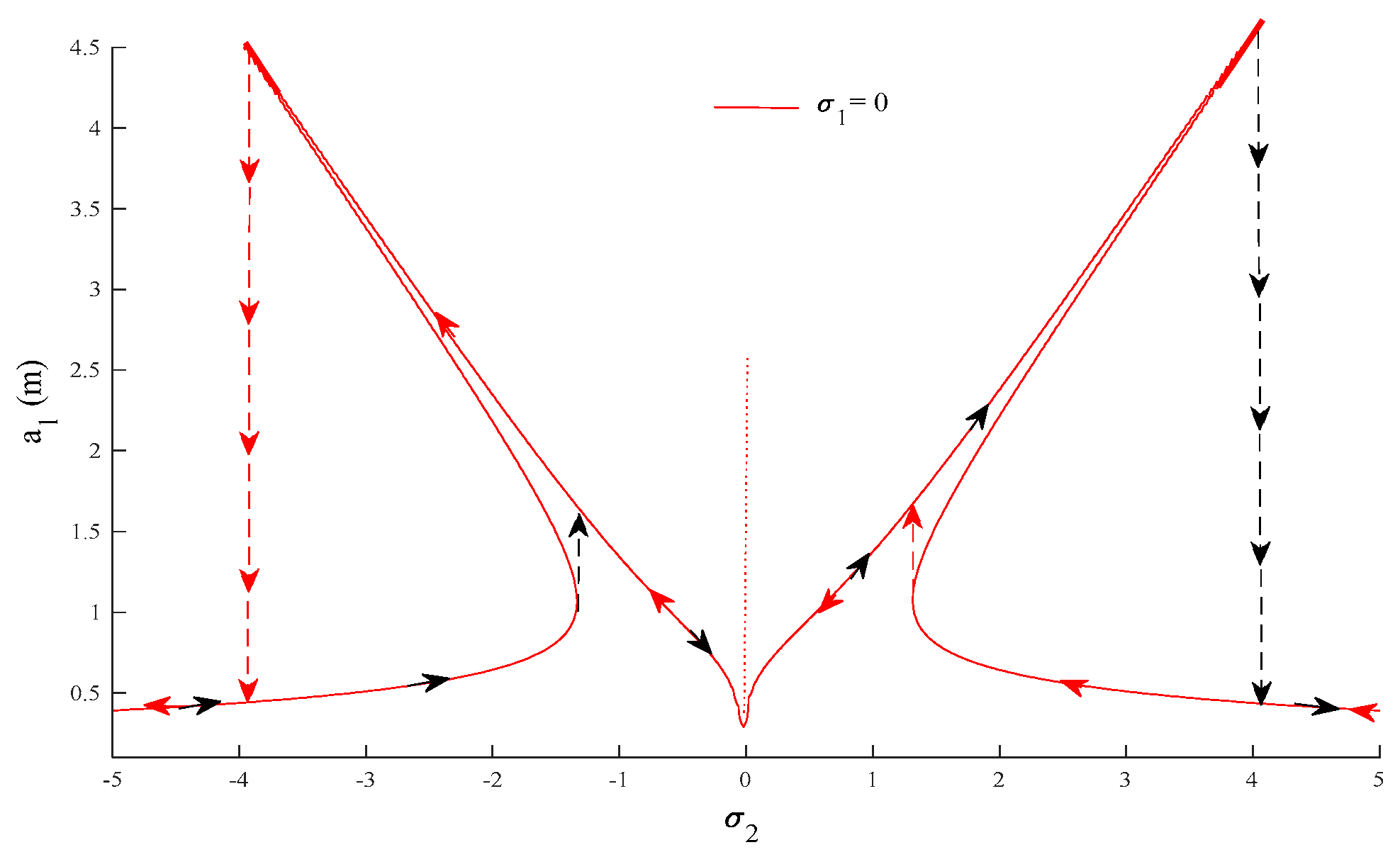
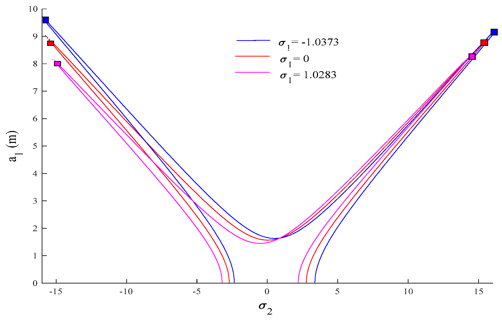
In forced oscillation, no matter the excitation forcing the sling or the beam, the amplitude–frequency response of the cable had an obvious jumping phenomenon. The amplitude–frequency response of the beam had a jumping phenomenon only when the excitation forced the sling. On the right side of the baseline, the responses of the sling and the beam both exhibited hardening behavior, while on the left side, they exhibited softening behavior. In the case of σ₁ = 0, the amplitude–frequency response curve was symmetrical along the baseline. When σ₁ > 0 and σ₁ < 0, the baseline slightly shifted to right and left, respectively, and the amplitude–frequency response curve was no longer symmetrical.

(3)

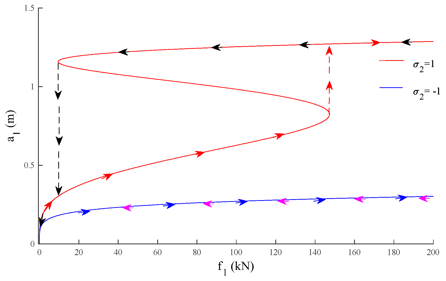
In forced oscillation, no matter the excitation forcing the sling or the beam, the amplitude–force response of the cable had an obvious jumping phenomenon. The amplitude–force response of the beam had a jumping phenomenon only when the excitation forced the sling. When the excitation forced the beam, the amplitude of the beam was independent of the excitation, which revealed that the saturation phenomenon existed.

(4)

In forced oscillation, no matter the excitation forcing the sling or the beam, the steady-state responses of the sling and the beam were not excited at the same time. When the excitation forced the sling, the sling was excited ahead of the beam, and when the excitation forced the beam, the beam was excited ahead of the sling.

References

1. Takahashi, K. Dynamic stability of cables subjected to an axial periodic load. J. Sound Vib. 1991, 144, 323–330. [Google Scholar] [CrossRef]
2. Pinto da Costa, A.; Martins, J.A.C.; Branco, F.A.; Lilien, J.L. Oscillations of bridge stay cables tby periodic motions of deck and/or towers. J. Eng. Mech. 1996, 122, 613–622. [Google Scholar]
3. Arafat, H.N.; Nayfeh, A.H. Non-linear responses of sus-pended cables to primary resonance excitations. J. Sound Vib. 2002, 266, 325–354. [Google Scholar] [CrossRef]
4. Ni, Y.Q.; Ko, J.M.; Zheng, G. Dynamic analysis of large- diameter sagged cables taking into account flexural rigidity. J. Sound Vib. 2002, 257, 301–319. [Google Scholar] [CrossRef]
5. Wu, Q.; Takahashi, T.; Okabayashi, T. Response charac-teristics of local vibrations in stay cables on an existing cable stayed bridge. J. Sound Vib. 2003, 261, 403–420. [Google Scholar] [CrossRef]
6. Perkins, N.C. Modal interactions in the non-linear response of elastic cables under parametric/external excitation. Int. J. Non Linear Mech. 1992, 27, 233–250. [Google Scholar] [CrossRef]
7. Lilien, J.L.; Pinto da Costa, A. Vibration amplitudes caused by parametric excitation of cable stayed structures. J. Sound Vib. 1994, 174, 69–90. [Google Scholar] [CrossRef]
8. Cai, Y.; Chen, S.S. Dynamics of elastic cable under para-metric and external resonances. J. Eng. Mech. 1994, 120, 1784–1802. [Google Scholar]
9. Warnitchai, P.; Fujino, Y. A non-linear dynamic model for cables and its application to a cable-structure system. J. Sound Vib. 1995, 187, 693–712. [Google Scholar] [CrossRef]
10. Benedettini, F.; Rega, G. Non-linear oscillations of a four-degree-of-freedom model of a suspended cable under multiple internal resonance conditions. J. Sound Vib. 1995, 182, 773–798. [Google Scholar] [CrossRef]
11. Caetano, E.; Cunha, A. Investigation of dynamic cable-deck interaction in a physical model of a cable-stayed bridge. Earthq. Eng. Struct. Dyn. 2000, 29, 499–521. [Google Scholar] [CrossRef]
12. Sun, B.N.; Wang, Z.G.; Ko, J.M. Cable oscillation induced by parametric excitation in cable-stayed bridges. J. Zhejiang Univ. Sci. 2003, 4, 13–20. [Google Scholar] [CrossRef] [PubMed]
13. Gattulli, V.; Morandini, M. A parametric analytical model for non-linear dynamics in cable-stayed beam. Earth Quake Eng. Struct. Dyn. 2002, 31, 1281–1300. [Google Scholar] [CrossRef]
14. Gattulli, V.; Lepidi, M. Nonlinear interactions in the planar dynamics of cable-stayed beam. Int. J. Solids Struct. 2003, 40, 4729–4748. [Google Scholar] [CrossRef]
15. Lenci, S.; Ruzziconi, L. Nonlinear phenomena in the single-mode dynamics of a cable-supported beam. Int. J. Bifurc. Chaos 2009, 19, 923–945. [Google Scholar] [CrossRef]
16. Gattulli, V.; Lepidi, M. One-to-two global-local interaction in a cable-stayed beam observed through analytical, finite element and experimental models. Int. J. Non Linear Mech. 2005, 40, 571–588. [Google Scholar] [CrossRef]
17. Amer, Y.A.; Hegazy, U. Chaotic vibration and resonance phenomenon in a parametrically excited string-beam coupled system. Mechanica 2012, 47, 969–984. [Google Scholar] [CrossRef]
18. Fujino, Y.; Warnitchai, P. An experimental and analytical study of auto parametric resonance in a 3-DOF model of cable-stayed-beam. Nonlinear Dyn. 1993, 4, 111–138. [Google Scholar] [CrossRef]
19. Lepidi, M.; Gattulli, V. Non-linear interactions in the flexible multi-body dynamics of cable-supported bridge cross-sections. Int. J. Non Linear Mech. 2016, 80, 14–28. [Google Scholar] [CrossRef]
20. Wu, Q.; Qi, G. Viscoelastic string-beam coupled vibro-impact system: Modeling and dynamic analysis. Eur. J. Mech. A Solids 2020, 82, 104012. [Google Scholar] [CrossRef]
21. Nicaise, S.; Hadjsaleh, M.B. Polynomial Stability of a Suspension Bridge Model by Indirect Dampings. Z. Für Anal. Und Ihre Anwend. 2021, 40, 367–400. [Google Scholar] [CrossRef]
22. Lenci, S.; Clementi, F.; Kloda, L.; Warminski, J.; Rega, G. Longitudinal–transversal internal resonances in Timoshenko beams with an axial elastic boundary condition. Nonlinear Dyn. 2021, 103, 3489–3513. [Google Scholar] [CrossRef]
23. Bilal, N.; Tripathi, A.; Bajaj, A.K. On experiments in harmonically excited cantilever plates with 1:2 internal resonance. Nonlinear Dyn. 2020, 100, 15–32. [Google Scholar] [CrossRef]
24. Guillot, V.; Givois, A.; Colin, M.; Thomas, O.; Ture Savadkoohi, A.; Lamarque, C.-H. Theoretical and experimental investigation of a 1:3 internal resonance in a beam with piezoelectric patches. J. Vib. Control 2020, 26, 1119–1132. [Google Scholar] [CrossRef]
25. Ying, H.; Gao, M.; Hu, Y.; Li, Y. Nonlinear Dynamic Analysis of Axially Moving Laminated Shape Memory Alloy Beam with 1:3 Internal Resonance. Materials 2021, 14, 4022. [Google Scholar]
26. Nikpourian, A.; Ghazavi, M.R.; Azizi, S. Size-dependent modal interactions of a piezoelectrically laminated microarch resonator with 3:1 internal resonance. Appl. Math. Mech. Engl. 2020, 41, 1517–1538. [Google Scholar] [CrossRef]
27. Hajjaj, A.Z.; Alfosail, F.K.; Jaber, N.; Ilyas, S.; Younis, M.I. Theoretical and experimental investigations of the crossover phenomenon in micromachined arch resonator: Part II—Simultaneous 1:1 and 2:1 internal resonances. Nonlinear Dyn. 2020, 99, 407–432. [Google Scholar] [CrossRef]
Figure 1. Configuration of the suspension system: (a) reference and (b) instantaneous.
Buildings 13 01319 g001
Figure 2. Amplitude–time responses a 1 t (a) and a 2 t (b) of free vibration without damping.
Buildings 13 01319 g002
Figure 3. Amplitude–time response a 1 t of free vibration with damping.
Buildings 13 01319 g003
Figure 4. Amplitude–time response a 2 t of free vibration with damping.
Buildings 13 01319 g004
Figure 5. Amplitude–time response v t of free vibration with (b) and without (a) damping.
Buildings 13 01319 g005
Figure 6. Amplitude–frequency response a 1 σ 2 of the excitation on the sling ( σ 1 = 0 ).
Buildings 13 01319 g006
Figure 7. Amplitude–frequency response a 2 σ 2 of the excitation on the sling ( σ 1 = 0 ).
Buildings 13 01319 g007
Figure 8. Amplitude–frequency response a 1 σ 2 of the excitation on the sling.
Buildings 13 01319 g008
Figure 9. Amplitude–frequency response a 2 σ 2 of the excitation on the sling.
Buildings 13 01319 g009
Figure 10. Amplitude–force response a 1 f 1 of the excitation on the sling.
Buildings 13 01319 g010
Figure 11. Amplitude–force response a 2 f 2 of the excitation on the sling.
Buildings 13 01319 g011
Figure 12. (a) Steady-state response of the sling and the beam when the excitation forces the sling ( σ 1 = 0, σ 2 = 1, f 1 = 30). (b) shows some details in (a).
Buildings 13 01319 g012
Figure 13. Steady-state response of the sling when the excitation forces the sling ( σ 1 = 0 , σ 2 = 2 ,   f 1 = 30 ).
Buildings 13 01319 g013
Figure 14. Steady-state response of the beam when the excitation forces the sling ( σ 1 = 0 , σ 2 = 2 ,   f 1 = 30 ).
Buildings 13 01319 g014
Figure 15. Amplitude–frequency response a 1 σ 2 of the excitation on the beam ( σ 1 = 0 ).
Buildings 13 01319 g015
Figure 16. Amplitude–frequency response a 2 σ 2 of the excitation on the beam ( σ 1 = 0 ).
Buildings 13 01319 g016
Figure 17. Amplitude–frequency response a 1 σ 2 of the excitation on the beam ( σ 1 = 0 ,   1.0283 ,   1.0373 ).
Buildings 13 01319 g017
Figure 18. Amplitude–frequency response a 2 σ 2 of the excitation on the beam ( σ 1 = 0 ,   1.0283 ,   1.0373 ).
Buildings 13 01319 g018
Figure 19. Amplitude–force response a 1 f 2 of the excitation on the beam.
Buildings 13 01319 g019
Figure 20. Steady-state response of the sling and the beam when the excitation forces the beam ( σ 1 = 0 , σ 2 = 1 , f 2 = 30   KN ).
Buildings 13 01319 g020
Figure 21. Steady-state response of the sling when the excitation forces the beam ( σ 1 = 0 ,   σ 2 = 4 ,   f 2 = 30   KN ).
Buildings 13 01319 g021
Figure 22. Steady-state response of the beam when the excitation forces the beam ( σ 1 = 0 ,   σ 2 = 4 ,   f 2 = 30   KN ).
Buildings 13 01319 g022
Disclaimer/Publisher’s Note: The statements, opinions and data contained in all publications are solely those of the individual author(s) and contributor(s) and not of MDPI and/or the editor(s). MDPI and/or the editor(s) disclaim responsibility for any injury to people or property resulting from any ideas, methods, instructions or products referred to in the content.