Article

Experimental Research on Motion Analysis Model and Trajectory Planning of GLT Palletizing Robot

1
Research Institute of Wood Industry, Chinese Academy of Forestry, Beijing 100091, China
2
Fujian Academy of Forestry, Fuzhou 350012, China
*
Author to whom correspondence should be addressed.
Buildings 2023, 13(4), 966; https://doi.org/10.3390/buildings13040966
Submission received: 1 March 2023 / Revised: 28 March 2023 / Accepted: 3 April 2023 / Published: 5 April 2023

Abstract

:
To improve wood structure processing efficiency, a palletizing robot suitable for loading and unloading glued laminated timber (GLT) has been developed. The robot comprises a six-axis connecting rod mechanism and a sponge sucker as a grasping actuator, which can enable the intelligent automatic loading and unloading and palletizing operations for small-sized GLT. Matlab robotics was used to construct the kinematic model of the GLT loading and unloading robot. Based on Matlab and Monte Carlo methods, the robot workspace was simulated and analyzed to determine the scope of the robot workspace. Using the high-order quintic and sixtic polynomial curve interpolation method, the trajectory of wood structure parts in the process of loading and unloading operations was planned, respectively, under the two conditions of staying and not staying. Tests verified that the simulation results of the pose of the end-effector were consistent with the actual pose of the robot. The robot’s working range could be analyzed intuitively and effectively. The robot’s operation trajectory planning provides data support and a parameter basis for the automatic control and program design of a loading, unloading and palletizing robot.

1. Introduction

Glued laminated timber (GLT) is one of the important products in the ecological timber industry chain, which can be widely used in wood structure construction, furniture, decoration and bridges. The GLT industry also plays a vital role in China’s employment-demand consumption industry and the national economy [1]. Several targeted industrial development plans have been issued with the acceleration of China’s ecological civilization process and the sustainable development of low-carbon industry. Applying GLT in the innovative development of prefabricated wood structure buildings represents a new opportunity to optimize the industrial development pattern of green buildings in China. However, with the diversified demands of wood structure customization, the quantity of glulam processing exponentially increases and the processing becomes more complex, as well as having low output and efficiency [2]. The development of intelligent automatic processing technology and equipment for glulam is comparatively lagging behind, which has become the main bottleneck to the promotion and application of modern wood structure buildings. Especially in the intelligent manufacturing and production of wood structures, the loading, unloading and palletizing links of GLT are mainly manual operations, which affects the production efficiency to a large extent.
Structural glued laminated timber has good performance, diverse types and a perfectly relevant standard system, which is usually used for load-bearing components in building structures. Domestic scholars have studied its physical structural properties [3,4], drilling processing properties [5], production process [6,7] and flexible drilling control system [8], which has accelerated the application of structural glued laminated timber in wood structure buildings in China. Scholars at home and abroad have explored and studied the integrated digital information manufacturing platform and software system of GLT [9], which provides a theoretical basis for intelligent manufacturing. With the wide application and promotion of industrial robots in industrial automation production, industrial robots have been applied in the intelligent manufacturing of GLT. By analyzing the process characteristics of plate processing, the layout of equipment and the running tracks of industrial robots are planned. Machine vision is used to quickly identify the position of plates, and an automatic loading and unloading system for a woodworking center is built [10]. The intelligent automatic loading and unloading palletizing technology and equipment of GLT is a key component of the intelligent manufacturing of wood structures, which can remove the need for a large portion of manual labor from heavy repetitive loading, unloading and palletizing operations, reduce labor intensity and improve production efficiency. Therefore, the study of the trajectory planning method and motion analysis model of a palletizing robot is of great significance to realize the intelligent manufacturing of wood structures.
In this paper, a six-axis robot was used, with a sponge sucker as the integrated material to grasp the actuator, for intelligent, automatic loading and unloading to improve the automation level and work efficiency. By constructing a robot kinematic model, the workspace of the robot was analyzed using the Monte Carlo method and Matlab based on a kinematic analysis. The robot’s automatic loading and unloading operation trajectory planning provides data support and a parameter basis for the automatic control and program design of a loading, unloading and palletizing robot.

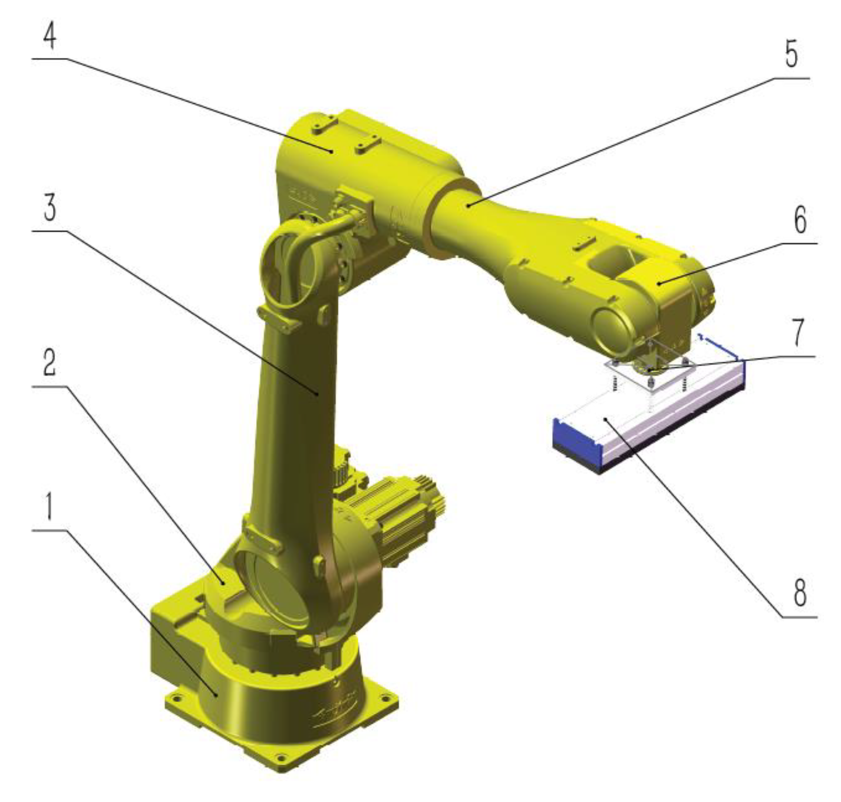
2. Overview of the GLT Palletizing Robot

GLTs are mostly wood boards and wood strips of various kinds and sizes. To meet the requirements of the integrated material loading and unloading palletizing operation, a 6-DOF, 6-axis robot with a multidimensional and comprehensive working space was equipped with a fixture. There are knots and air permeability on the surface of soft GLT, and a mechanical clamping fixture can easily cause damage to the surface of the material. A traditional vacuum suction cup cannot effectively form a confined space on the surface of the material and easily discharges during operation, which cannot sufficiently adapt to the automatic loading and unloading of GLT. Therefore, through the comprehensive analysis of various vacuum suction cup performances, principles and vacuum system control methods [11,12], the internal check valve sponge suction cup vacuum generator was chosen as the integrated material loading and unloading capture actuator.
The wooden structure palletizing robot was composed of a base, a waist connecting rod, a large arm connecting rod, an elbow connecting rod, a small arm connecting rod, a wrist connecting rod, a rotary flange and an end effector. Each connecting rod was composed of a servo motor, an encoder and a transmission mechanism. The end-effector was composed of a connecting plate, a spring, a screw and a sponge sucker. The structure is shown in Figure 1.

3. Kinematic Analysis

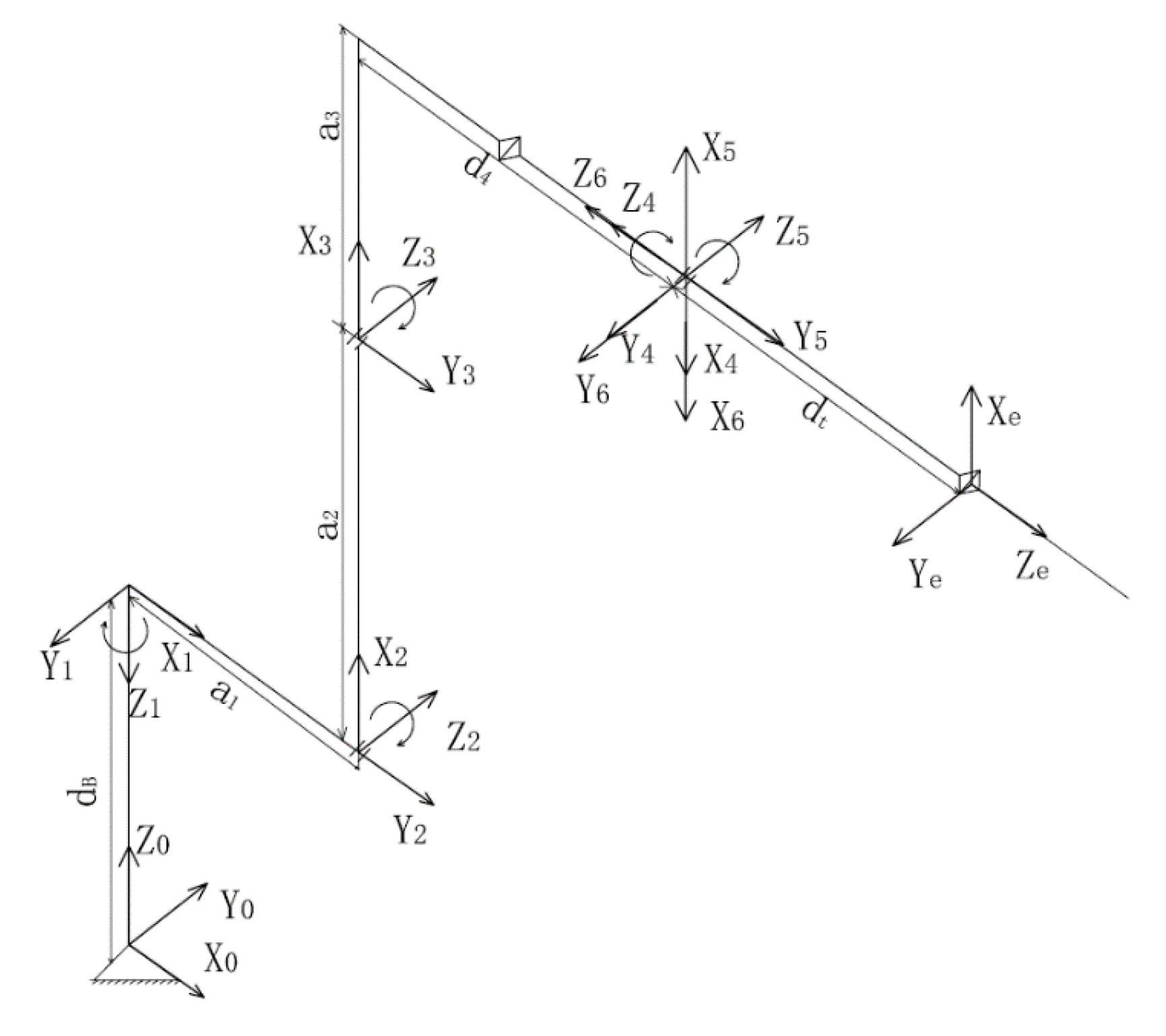
3.1. Establishment of Coordinate System and Determination of D-H Parameters

In order to facilitate the complex geometry of each link of the robot, it was necessary to set a link coordinate system on each link to describe the relationship of the coordinate system between these links. The relative relationship between the joints, as well as the function between the end-effector position and the operation base frame, were studied.
The link was numbered from the fixed base (link 0) of the robot. The first movable link was named link 1, and using this method, the terminal link of the robot was used as link 6. The convention was established according to Craig’s reference coordinate system [13,14], and the coordinate Z-axis and origin of each robot arm were established on the axis in front of the arm. Except for the first and sixth links, the axis of each link was normal, which is the common normal of the front and rear adjacent links. The robot’s connecting rod coordinate system is shown in Figure 2:
According to the Denavit–Hartenberg method [15], D-H parameters of each connecting rod were determined, and the D-H parameters are shown in Table 1.

3.2. Forward Kinematics

Four homogeneous transformations were used from the position of connecting rod i−1 to rod i. Firstly, the {i−1} coordinate system was rotated around the xi−1 axis αi−1 angle so that the zi−1 axis rotated in the same direction as the zi axis. Then, the ai−1 distance was translated along the xi−1 axis and the coordinate system was moved to the i axis, and then, it rotated around the zi axis θi angle. Finally, the d distance of translation along the zi axis coincided with the coordinate system {i} of i bar [16,17]. The transformation from coordinate {i−1} to coordinate {i} could be realized by using Equation (1).
T i i 1 = R o t x , α i 1 T r a n s α i 1 , 0 , 0 R o t z , θ i T r a n s 0 , 0 , d i
Formula (2) was used, which could be calculated from four transformation matrices.
  T i i 1 = c θ i s θ i 0 a i 1 s θ i c α i 1 c θ i c α i 1 s α i 1 d i s α i 1 s θ i s α i 1 c θ i s α i 1 c α i 1 d i c α i 1 0 0 0 1
where c = cos and s = sin.
Substituting the robot D-H parameters into Equation (2), we could obtain:
T 1 0 = c θ 1 s θ 1 0 0 s θ 1 c θ 1 0 0 0 0 1 0 0 0 0 1
T 2 1 = c θ 2 s θ 2 0 149.078 0 0 1       0 s θ 2 c θ 2 0 0 0 0 0 1
T 3 2 = c θ 3 s θ 3 0 790.385 s θ 3 c θ 3 0 0 0 0 1 0 0 0 0 1
T 4 3 = c θ 4 s θ 4 0 150.305 0 0 1 860.711 s θ 4 c θ 4 0 0 0 0 0 1
T 5 4 = c θ 5 s θ 5 0 0 0 0 1 0 s θ 5 c θ 5 0 0 0 0 0 1
  T 6 5 = c θ 6 s θ 6 0 0 0 0 1 0 s θ 6 c θ 6 0 0 0 0 0 1
T       6 0 = T 1 0 T 2 1 T 3 2 T 4 3 T 5 4 T 6 5
The robot base had a fixed transformation to Z relative to the workpiece reference system along the Z1 axis dB. The end of the axial robot tool had a fixed transformation E relative to the wrist’s end coordinate {6}. Firstly, dt was translated along the Z6 axis and then rotated around the Ye axis θe [18,19]. The transformation TT of the robot tool end relative to the workpiece reference system is:
TT = Z T 6 0 E  
Z = T r a n s 0 , 0 , d B = 1 0 0 0 0 1 0 0 0 0 1 d B 0 0 0 1
E = R o t Y e , p i T r a n s 0 , 0 , d t = C θ e 0 S θ e 0 0 1 0 0 S θ e 0 C θ e 0 0 0 0 1 1 0 0 0 0 1 0 0 0 0 1 d t 0 0 0 1
The robot kinematics equation X is:
T T = Z T 6 0 E = r 11 r 12 r 13 p x r 21 r 22 r 23 p y r 31 r 32 r 33 p z 0 0 0 1
The homogeneous transformation matrix of Equations (3)–(6) was substituted into Equation (7), and then, Equation (8) could be obtained:
r 11 = s 6 ( c 4 s 1 + s 4 ( c 1 s 2 s 3 c 1 c 2 c 3 ) ) c 6 ( c 5 ( s 1 s 4 c 4 ( c 1 s 2 s 3 c 1 c 2 c 3 ) ) + s 5 ( c 1 c 2 s 3 + c 1 c 3 s 2 ) ) r 12 = c 6 ( c 4 s 1 + s 4 ( c 1 s 2 s 3 c 1 c 2 c 3 ) ) s 6 ( c 5 ( s 1 s 4 c 4 ( c 1 s 2 s 3 c 1 c 2 c 3 ) ) + s 5 ( c 1 c 2 s 3 + c 1 c 3 s 2 ) ) r 13 =   c 5 ( c 1 c 2 s 3   + c 1 c 3 s 2 ) s 5 ( s 1 s 4 c 4 ( c 1 s 2 s 3 c 1 c 2 c 3 ) ) r 21 = s 6 ( c 1 c 4 + s 4 ( c 2 c 3 s 1 s 1 s 2 s 3 ) ) c 6 ( c 5 ( c 1 s 4 c 4 ( c 2 c 3 s 1 s 1 s 2 s 3 ) ) s 5 ( c 2 s 1 s 3 + c 3 s 1 s 2 ) ) , r 22 = c 6 ( c 1 c 4 + s 4 ( c 2 c 3 s 1 s 1 s 2 s 3 ) ) s 6 ( c 5 ( c 1 s 4 c 4 ( c 2 c 3 s 1 s 1 s 2 s 3 ) ) s 5 ( c 2 s 1 s 3 + c 3 s 1 s 2 ) ) r 23 = s 5 ( c 1 s 4 c 4 ( c 2 c 3 s 1 s 1 s 2 s 3 ) ) c 5 ( c 2 s 1 s 3 + c 3 s 1 s 2 ) r 31 =   s 23 s 4 s 6 c 6 ( c 23 s 5 s 23 c 4 c 5 ) r 32 = s 6 ( c 23 s 5 s 23 c 4 c 5 )   s 23 c 6 s 4 r 33 =   c 23 c 5 + s 23 c 4 s 5 p x =   a 2 c 1 + a 4 c 23 c 1 + d 4 s 23 c 1 + a 3 c 1 c 2 d t s 23 c 1 c 5 + d t s 1 s 4 s 5 + d t c 1 c 2 c 3 c 4 s 5 d t c 1 c 4 s 2 s 3 s 5 p y =   d t s 23 c 5 s 1 a 4 c 23 s 1 d 4 s 23 s 1 a 3 c 2 s 1 a 2 s 1 + d t c 1 s 4 s 5 d t c 2 c 3 c 4 s 1 s 5 + d t c 4 s 1 s 2 s 3 s 5 p z =   d b   + d 4 c 23     a 4 s 23     a 3 s 2     d t s 23 s 45 / 2 d t c 23 c 5 + d t   s 4 - 5 s 23 / 2
where c i = cos θ i , s i = sin θ i , c i j = cos ( θ i + θ j ) , s i j = sin ( θ i + θ j ) ,     s i j = sin ( θ i θ j )

4. Matlab Simulation of Robot

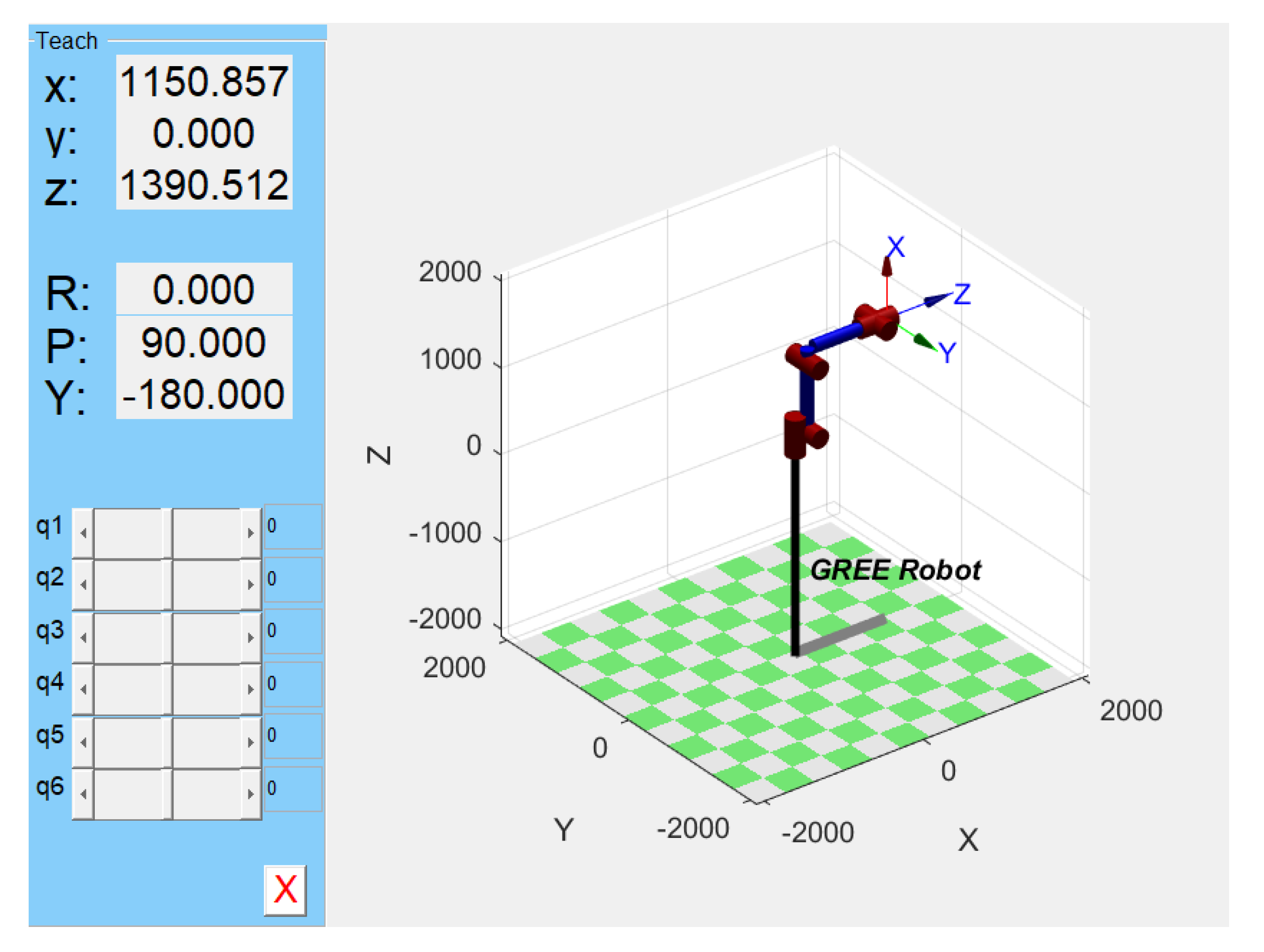
4.1. Model Establishment

The Matlab Robotics Toolbox is a set of Matlab-based robotics toolboxes developed and maintained by the Australian scientist, Peter Corke; it contains many important functions such as kinematics, dynamics and trajectory planning in robotics research [20]. It can conduct a graphic simulation of a robot and analyze the test data results of real robot control. The Link function in Matlab robotics was used to build the robot connecting rod, and the six connecting rods were connected by the SerialLink function to build the simulation model of the robot [21]. Industrial robot modeling procedures are as follows:
clear;clc;clf;
th(1) = 0; d(1) = 0; a(1) = 0; alp(1) = pi;
th(2) = −pi/2; d(2) = 0; a(2) = 149.078; alp(2) = pi/2;
th(3) = 0; d(3) = 0; a(3) = 790.385; alp(3) = 0;
th(4) = pi; d(4) = −860.711; a(4) = 150.305; alp(4) = pi/2;
th(5) = pi; d(5) = 0; a(5) = 0; alp(5) = pi/2;
th(6) = pi; d(6) = 0; a(6) = 0; alp(6) = pi/2;
L1 = Link([th(1), d(1), a(1), alp(1), 0], ‘modified’);
L2 = Link([th(2), d(2), a(2), alp(2), 0], ‘modified’); L2.offset = −pi/2;
L3 = Link([th(3), d(3), a(3), alp(3), 0], ‘modified’);
L4 = Link([th(4), d(4), a(4), alp(4), 0], ‘modified’);L4.offset = pi;
L5 = Link([th(5), d(5), a(5), alp(5), 0], ‘modified’);L5.offset = pi;
L6 = Link([th(6), d(6), a(6), alp(6), 0], ‘modified’);L6.offset = pi;
robot = SerialLink([L1, L2, L3, L4, L5, L6]);
robot.name = ‘GREE Robot’;
robot.display();
robot.base = transl(0,0,449.822);
robot.tool = transl(0 ,0 ,-141.068)*troty(pi);
robot.teach();
The 3D simulation model of the robot is shown in Figure 3:

4.2. Forward Kinematics Simulation Verification

Within the allowable range of joint variables, three groups of joint variables were randomly set, and the robot model established in Matlab was used for the simulation to obtain the position (X, Y, Z) and attitude (R, P, Y) of the end effector. Three sets of variable values were calculated into the industrial robot equation, and the end effector’s position (X, Y, Z) and attitude (R, P, Y) were calculated. The forward kinematics equation was verified by comparing the three groups of variables. The comparison results of the kinematics equation and simulation calculation of the end effector’s attitude are shown in Table 2.

4.3. Inverse Kinematics Simulation Verification

The inverse kinematics of a robots is a method to solve the motion equation. The desired posture was achieved by giving the geometric parameters of the robot link and the desired position and attitude (posture) of the robot’s end effector relative to the reference coordinate system and the joint variables. When the work task was described by the Cartesian coordinate system, the above provisions had to be transformed into a series of joint variables that the arm could drive. Therefore, the solution of joint variables to determine the position and posture of the arm was the solution of the motion equation. The problem of solving the robot motion equation, inverse kinematics, was problem synthesis. The transformation matrix T of the pose of the robot’s end effector corresponding to the reference coordinate system in Table 2 was verified via inverse kinematic simulation using the ikine function qi=ikine (robot, TT) in Matlab robotics. The triple transformation matrix is provided as Equations (14)–(16).
T T 1 = 0.4670 0.5522 0.6907 783.71 0.3022 0.6344 0.7115 336.47 0.8310 0.5410 0.1294 323.58 0 0 0 1
T T 2 = 0.5808 0.8067 0.1094 15.43 0.7690 0.4996 0.3987 775.88 0.2670 0.3157 0.9105 157.17 0 0 0 1
T T 3 = 0.7771 0.1712 0.6056 1842.03 0.2301 0.8184 0.5265 74.28 0.5858 0.5485 0.5966 329.72 0 0 0 1
The simulation results of the inverse kinematic equations are shown in Table 3:
The rotation angles of each joint in the three groups of positions and postures of the robot’s end effector obtained from the simulation were consistent with the results of the joint variable parameters assumed in the forward kinematics simulation in Table 2, which validated the robot kinematics model.

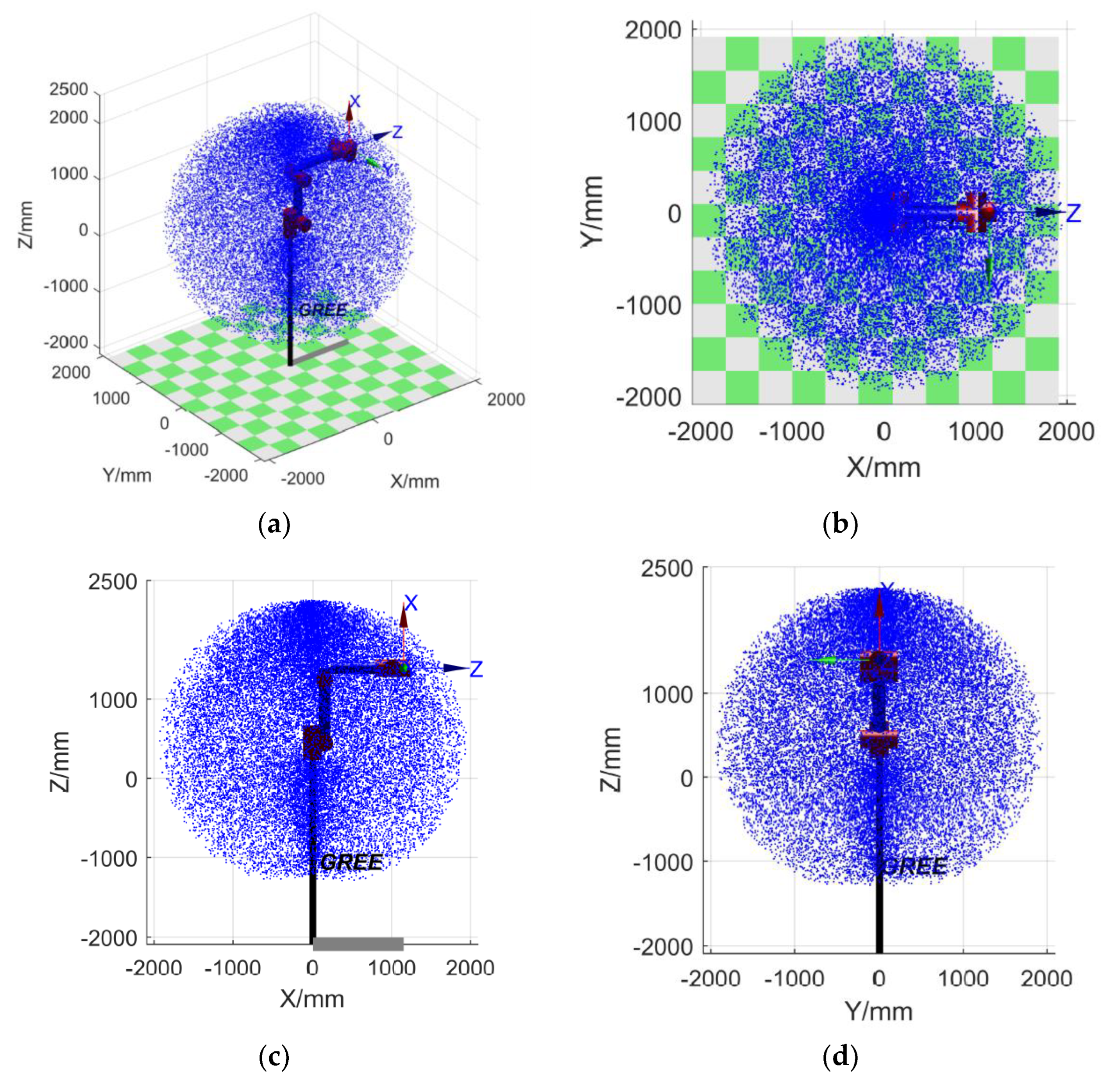
5. Simulation Verification and Solution of Working Space

A robot’s working space is the geometric locus of all possible coordinates of the center point of the end effector, which is one of the main indicators of a robot’s design. It reflects the working ability when performing a specific task, the working space range of the attitude of the end effector, and also the basis for the robot’s position arrangement in the production line and the operator’s safe working space to avoid being injured by the robot [22,23,24].
According to Formula (4), the position point coordinates of the robot’s end effector [px,py,pz]T can be obtained, which are only related to the relevant kinematic parameter, θi, and the point set of the robot’s working space is P.
P = x , y , z x = f x θ 1 , θ 2 , θ 3 , θ 4 , θ 5 , θ 6 y = f y θ 1 , θ 2 , θ 3 , θ 4 , θ 5 , θ 6 z = f z θ 1 , θ 2 , θ 3 , θ 4 , θ 5 , θ 6 θ m i n θ i θ m a x i = 1 , 2 , 3 , 4 , 5 , 6
After randomly selecting within the rotation range of each joint of the robot θi (i = 1,2,3,4,5,6) and substituting it into Formula (6), the working space point set of the center point of the robot’s end effector could be obtained.
The calculation of the robot kinematics equation was large, and the design and analysis were complicated. In order to solve this problem, Matlab robotics 2016b software was used for robot simulation modeling. According to the Monte Carlo method, the random variables of each joint were generated as well as the group of joint space vectors of the manipulator. Through calculating the forward kinematics solution, the working space distribution cloud map was drawn from the joint space to the working space at the end (Cartesian coordinate system) [25,26].
According to the Monte Carlo numerical analysis method, 30,000 groups within each joint range θi (i = 1,2,3,4,5,6) value were randomly selected by the Matlab rand function and then substituted into Equation (6) in turn to carry out 30,000 iterative operations. After that, the corresponding coordinate set of the central point of the corresponding end effector was obtained. The point set formed by drawing all points in the three-dimensional coordinates was the robot working space cluster.
The Matlab program code is as follows:
clear;clc;clf;
th(1) = 0; d(1) = 0; a(1) = 0; alp(1) = pi ;
th(2) = −pi/2; d(2) = 0; a(2) = 149.078; alp(2) = pi/2;
th(3) = 0; d(3) = 0; a(3) = 790.385; alp(3) = 0;
th(4) = pi; d(4) = −860.711; a(4) = 150.305; alp(4) = pi/2;
th(5) = pi; d(5) = 0; a(5) = 0; alp(5) = pi/2;
th(6) = pi; d(6) = 0; a(6) = 0; alp(6) = pi/2;
L1 = Link([th(1), d(1), a(1), alp(1), 0], ‘modified’); L1.qlim = [−178,178]/180*pi;
L2 = Link([th(2), d(2), a(2), alp(2), 0], ‘modified’); L2.offset = −pi/2; L2.qlim = [−98,158]/180*pi;
L3 = Link([th(3), d(3), a(3), alp(3), 0], ‘modified’); L3.qlim = [−178,78]/180*pi;
L4 = Link([th(4), d(4), a(4), alp(4), 0], ‘modified’);L4.offset = pi; L4.qlim = [−400,400]/180*pi;
L5 = Link([th(5), d(5), a(5), alp(5), 0], ‘modified’);L5.offset = pi; L5.qlim = [−120,120]/180*pi;
L6 = Link([th(6), d(6), a(6), alp(6), 0], ‘modified’);L6.offset = pi; L6.qlim = [−500,500]/180*pi;
robot = SerialLink([L1, L2, L3, L4, L5, L6]);
robot.name = ‘GREE Robot’;
robot.display();
robot.base = transl(0,0,449.822);
robot.tool = transl(0,0,−141.068)*troty(pi);
robot.teach();
num = 30,000;
P = zeros(num,3);
for i = 1:num
q1 = L1.qlim(1) + rand*(L1.qlim(2)−L1.qlim(1));
q2 = L2.qlim(1) + rand*(L2.qlim(2)−L2.qlim(1));
q3 = L3.qlim(1) + rand*(L3.qlim(2)−L3.qlim(1));
q4 = L4.qlim(1) + rand*(L4.qlim(2)−L4.qlim(1));
q5 = L5.qlim(1) + rand*(L5.qlim(2)−L5.qlim(1));
q6 = L6.qlim(1) + rand*(L6.qlim(2)−L6.qlim(1));
q = [q1 q2 q3 q4 q5 q6];
T = robot.fkine(q);
P(i,:) = transl(T);
end
plot3(P(:,1),P(:,2),P(:,3),’b.’,’markersize’ ,2);
xlabel(‘X/m’);
ylabel(‘Y/m’);
zlabel(‘Z/m’);
hold on;
The cloud map of the robot’s working space is shown in Figure 4:

6. Robot Planning for Loading and Unloading Path of GLT

Robot trajectory planning was used to plan the trajectory of the robot’s motion and generate the operation trajectory in joint space and Cartesian space based on the kinematics and dynamics of the manipulator. The so-called trajectory refers to the displacement, velocity and acceleration of the manipulator’s joints in the movement. Trajectory planning calculated the expected trajectory according to the task’s requirements. During the robot trajectory planning, the task, motion path and trajectory of the robot were firstly described. Then, the target pose of the gripper was given to determine the path point, duration, motion speed and other trajectory parameters to reach the target. Finally, for the trajectory described internally, the robot movement’s displacement, velocity and acceleration were calculated in real time to generate the trajectory. The manipulator is usually regarded as the movement of the tool coordinate system relative to the working coordinate system. The point mentioned in trajectory planning refers to the position and attitude of the manipulator’s tool coordinate system, which was used to describe the state of the starting position, the path position and the target position of the robot during the operation process. There are two common trajectory planning methods of manipulators: in the first method, the position, velocity and acceleration on the selected transition node (interpolation point) is given a set of explicit constraints to achieve the continuity and smoothness of the operation, the use of polynomial curve function, the node interpolation and meet the constraints. In the second method, the analytical expression of the motion path is given, such as the straight path in Cartesian coordinate space, and then, a trajectory is determined in joint space or Cartesian coordinate space to approximate the predetermined path. In the first method, constraint setting and trajectory planning are carried out in joint space; so, a collision with obstacles may occur. The path constraints of the second method are given in Cartesian coordinate space, while the joint driver is controlled in joint space. Therefore, to obtain a trajectory close to the given path, the Cartesian coordinate path constraints must be first converted into joint coordinate path constraints via the function approximation method, and then, the parameterized path should be determined and the joint path constraints should be satisfied.

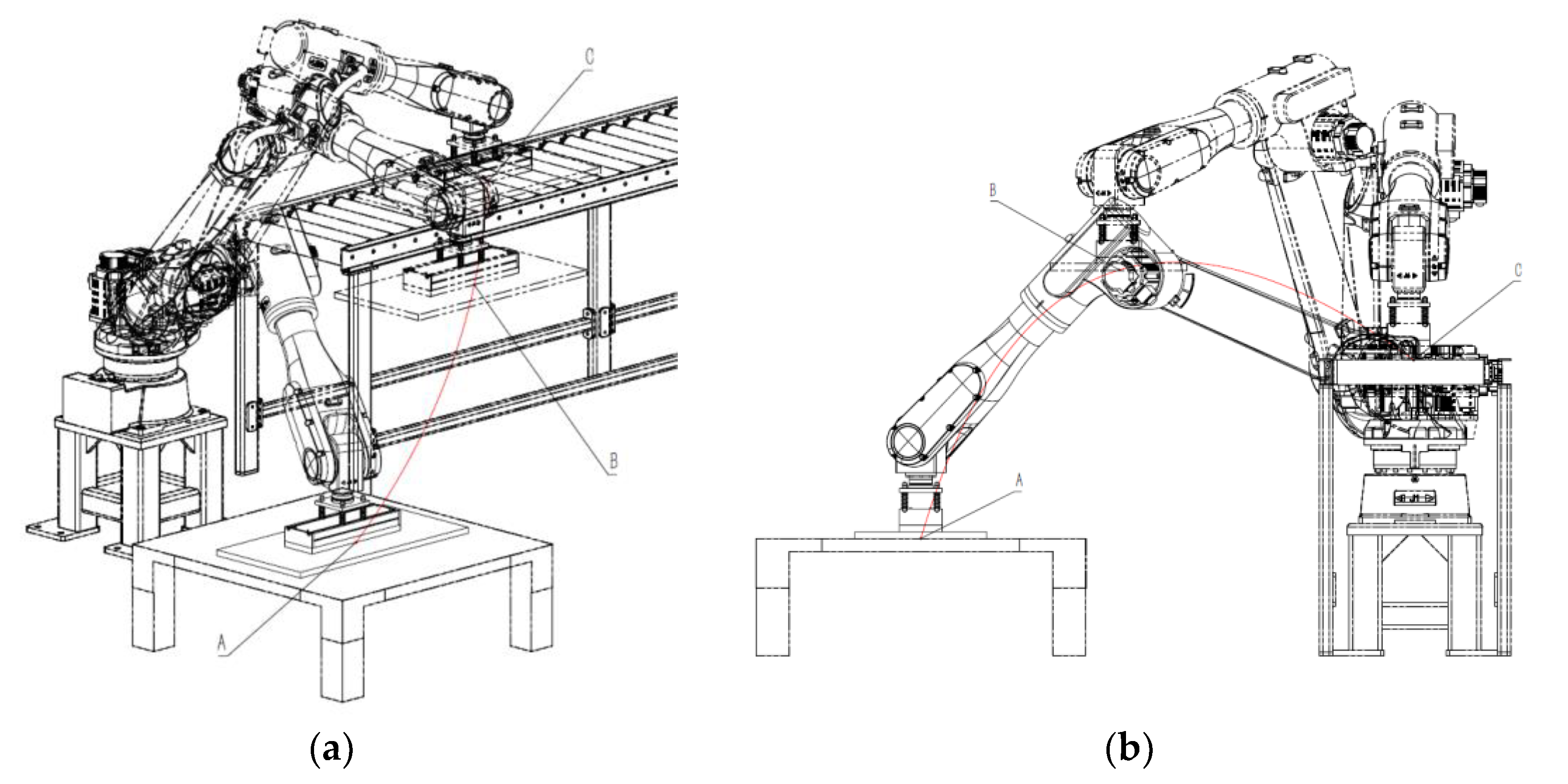
6.1. The Robot Makes Route Planning for the Loading and Unloading Operation of GLT

The robot’s loading and unloading trajectory of GLT refers to the displacement, velocity and acceleration of each joint of the robot when the end effector (sponge sucker) moved the GLT from the grasping position to the unloading position. The loading and unloading trajectory planning calculated the expected motion trajectory based on the analysis of dynamics when the robot was loading and unloading so that the robot could complete the loading and unloading operation continuously, smoothly and accurately. Because the loading and unloading operation position of GLT is a point-to-point operation, there was no more requirement for the trajectory in the process; so, the trajectory planning was carried out in the joint space [27]. When the robot was loading and unloading, it grabbed GLT from the tray and then placed it on the conveyor line through the critical path. In the process of movement, due to the height difference between the tray and the conveying line and the large size of GLT, GLT could have easily collided with the conveying line. It was necessary to plan the robot’s loading and unloading operation path. The robot grabbed the GLT from the tray at point A and then moved along curve AB to point B. The schematic diagram of the path planning is shown in Figure 5. At point B, the position of GLT was higher than the conveying line, and there was no collision between the GLT edge and the conveying line. After passing point B, the GLT was placed at point C of the conveyor line along the BC curve to complete the loading operation of grabbing it from the tray and placing it on the conveyor line. In the unloading operation of GLT, the robot held the integrated material at point C and moved along the CBA curve to point A to complete the feeding operation. The loading operation was the same as the unloading operation path, but the direction of movement was opposite. The trajectory planning method was the same. Therefore, this paper only carried out the trajectory planning for the feeding operation.
The coordinates of the path’s key points A, B and C are shown in Table 4.

6.2. Loading Operation Trajectory Planning

Common robot trajectory planning currently includes trapezoidal programming, parabolic programming, polynomial programming and S-type programming [28]. Quintic polynomial programming is most commonly used in polynomial programming and is widely used in robot trajectory planning. The acceleration discontinuity of trapezoidal programming and S-type programming will have a mechanical impact on the robot. In contrast, quintic polynomial programming is relatively mature in the transition planning method, which can ensure the continuity of displacement, velocity, acceleration and acceleration during the robot movement [29]. Therefore, the high-order quintic polynomial interpolation trajectory method was used to complete the trajectory planning. Not only was the tracking accuracy of the planned trajectory ensured, but it also could ensure continuous smooth displacement, velocity and acceleration in the process of moving. Finally, the machine ran smoothly, reducing the impact vibration and effectively extending the machine’s service life [30]. However, when the quintic polynomial was used to interpolate the points through multiple paths, some acceleration points still had the problem of abrupt change, which could have easily caused vibration. Therefore, the high-order sixth-degree polynomial interpolation can be used to realize continuous flat smoothing with extra speed in multipoint piecewise path planning.
According to the actual work requirements of the loading and unloading operations, there are two main situations. One is that when the sponge sucker absorbs the aggregate material during the loading and unloading operation, it is necessary to stay at the passing point to avoid obstacles and align the loading and unloading position. That is, the speed and acceleration are zero at the critical nodes of each path. Second, when the sponge sucker absorbs the aggregate material for the loading and unloading operation, avoiding obstacles and aligning the taking and discharging position is unnecessary. Each passing point does not need to stay. That is, the speed and acceleration are not zero at the critical node of each path. In this paper, the quintic polynomial interpolation method and high-order sixtic polynomial interpolation method were used to study the GLT loading and unloading operation trajectory planning, respectively.

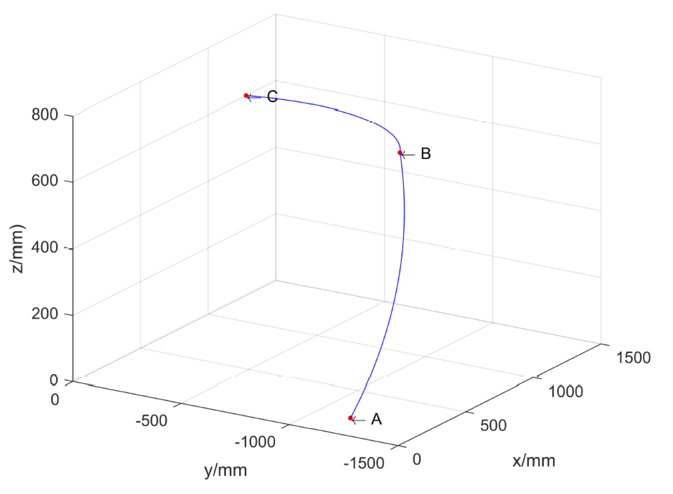
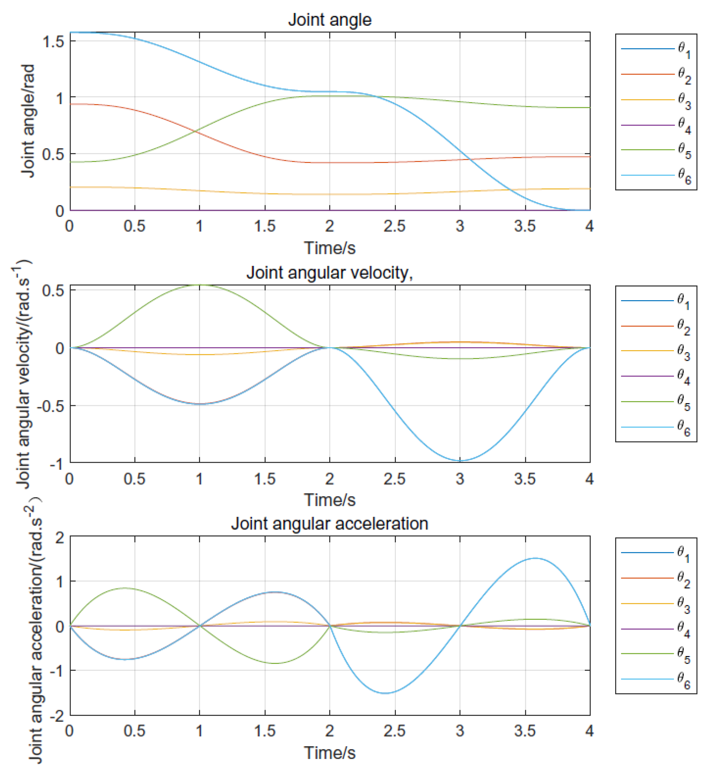
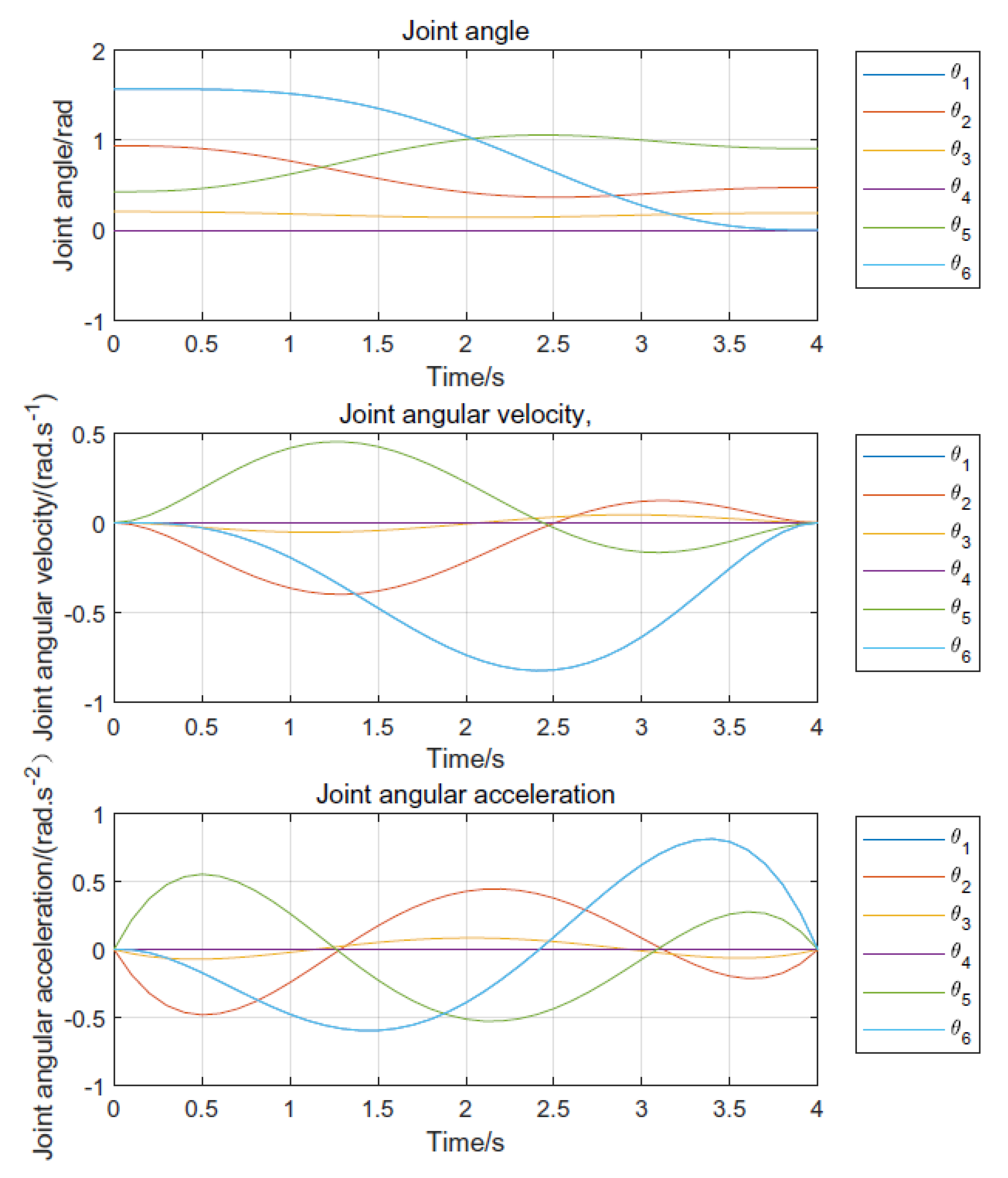
6.2.1. Loading Trajectory Planning Using High-Order Quintic Polynomial Interpolation

Because the sponge sucker will stay at the trajectory path point when gripping GLT for loading operation, the AB and BC sections can be independently planned using the quintic polynomial interpolation method for the loading and unloading operation path [31]. The general formula of trajectory planning for quintic polynomial interpolation is:
θ i t = a 0 + a 1 t + a 2 t 2 + a 3 t 3 + a 4 t 4 + a 5 t 5
The starting point of the feeding operation path is A, the passing point is B, and the target point is C. The pose state of the three points is shown in Table 4. Suppose the starting point position of each joint i is θ A , the path point position is θ B , the target point position is θ C , the starting point velocity is v A , the path point velocity is v B , the target point velocity is v c , the starting point acceleration is a A , the path point acceleration is a B , the target point acceleration is a C , the starting point time is t A , the path point time is t B and the target point time is t C . The kinematic parameters of each joint i in AB and BC are shown as Equations (19) and (20).
θ A = a 10 + a 11 t A + a 12 t A 2 + a 13 t A 3 + a 14 t A 4 + a 15 t A 5 v A = a 11 + 2 a 12 t A + 3 a 13 t A 2 + 4 a 14 t A 3 + 5 a 15 t A 4 a A = 2 a 12 + 6 a 13 t A + 12 a 14 t A 2 + 20 a 15 t A 3 θ B = a 10 + a 11 t B + a 12 t B 2 + a 13 t B 3 + a 14 t B 4 + a 15 t B 5 v B = a 11 + 2 a 12 t B + 3 a 13 t B 2 + 4 a 14 t B 3 + 5 a 15 t B 4 a B = 2 a 12 + 6 a 13 t A + 12 a 14 t A 2 + 20 a 15 t A 3
θ B = a 20 + a 21 t B + a 22 t B 2 + a 23 t B 3 + a 24 t B 4 + a 25 t B 5 v B = a 21 + 2 a 22 t B + 3 a 23 t B 2 + 4 a 24 t B 3 + 5 a 25 t B 4 a B = 2 a 22 + 6 a 23 t A + 12 a 24 t A 2 + 20 a 25 t A 3 θ C = a 20 + a 21 t C + a 22 t C 2 + a 23 t C 3 + a 24 t C 4 + a 25 t C 5 v c = a 21 + 2 a 22 t C + 3 a 23 t C 2 + 4 a 24 t C 3 + 5 a 25 t C 4 a C = 2 a 22 + 6 a 23 t C + 12 a 24 t C 2 + 20 a 25 t C 3
It is known that θ A , θ B , θ C , v A = v B = v c = 0 , a A = a B = a C = 0 . The time from point A to point B and from point B to point C is 2 s. By substituting each constraint into Equations (8) and (9), we can find that the quintic multiple of AB and BC is   θ 1 t , θ 2 t . The specific expression is shown in Equation (21).
θ 1 t = θ A + 5 θ B θ A 4 t 3 15 θ B θ A 16 t 4 + 3 θ B θ A 16 t 5   θ 2 t = θ B + 5 θ C θ B 4 t 3 15 θ C θ B 16 t 4 + 3 θ C θ B 16 t 5
We substituted the coordinates and positions of the three key points of A, B and C of the loading operation into the quintic polynomial (21) to obtain the feeding trajectory and the displacement, velocity and acceleration curves of the six joints, as shown in Figure 6 and Figure 7. During the loading operation, the curve from points A to B and C was continuous and smooth without abrupt changes, but the entire ABC curve was continuous at point B, but not smooth. This is because during the loading process, it stayed at point B and then moved to point C, and the trajectory was planned by two different quintic polynomials in two segments.
As shown in Figure 7, starting from point A, the displacement of the six joints of the robot increased steadily with time and gradually tended to be stable, and the range of joint displacement was all within the action range of the robot. The velocity of the robot’s six joints accelerated from t = 0 s, reached the peak velocity at t = 1 s and t = 3 s, and then decreased to 0 at t = 2 s and t = 4 s. Each joint’s acceleration and deceleration time were equal, and the range of the velocity change was within the range of the speed of each joint. The acceleration of each robot joint first increased from 0 to the maximum value, then decreased to 0, then continuously decreased from 0 to the minimum acceleration, and finally increased to 0. The running time of the increasing and decreasing positive and negative acceleration stages was equal.
Although the ABC operation track curve was not smooth at point B in the three-dimensional space during the loading process, the displacement, velocity and acceleration curves of the robot’s six joints were continuous, smooth and flexible without sudden changes, jumps, discontinuities and other conditions. This indicated that the robot operated smoothly during loading, without adverse conditions such as impact and large vibration. Therefore, the higher-order quintic polynomial interpolation method applied to the loading operation trajectory planning under the condition of staying at path point B.

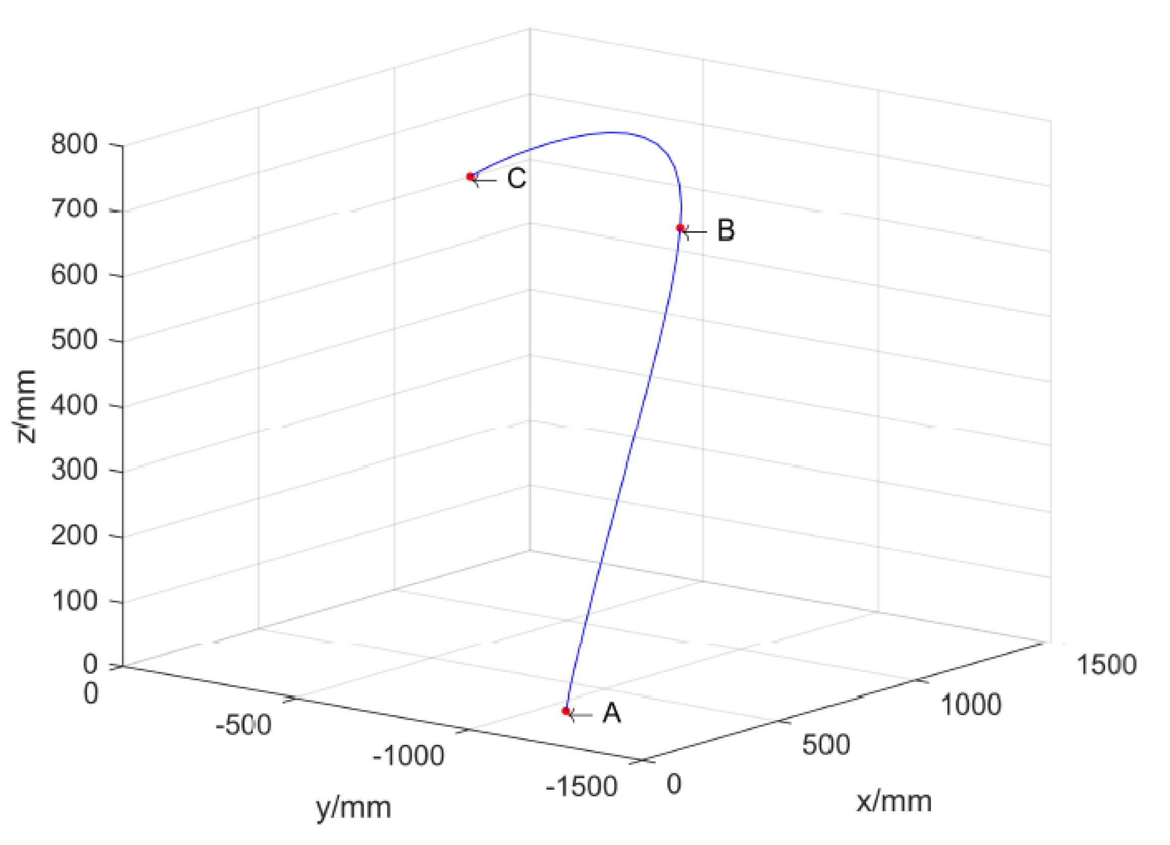
6.2.2. Loading and Unloading Trajectory Planning Using High-Order Six-Order Polynomial Interpolation

During the loading operation of the sponge sucker absorbing GLT, it did not stay at the passing point B. The AB section and BC section could be unified, and the six-order polynomial interpolation method could be used for the loading operation path planning. The general formula of six-degree polynomial interpolation trajectory planning is formula (22):
θ i t = a 0 + a 1 t + a 2 t 2 + a 3 t 3 + a 4 t 4 + a 5 t 5 + a 6 t 6
We substituted the constraints, such as θ A , θ B , θ C , v A = v c = 0 , v B , a A = a C = 0 , a B , and the time from point A to point B and from point B to point C into Equation (22), as shown in (23).
θ A = a 0 v A = a 1 a A = 2 a 2     θ B = a 0 + a 1 t B + a 2 t B 2 + a 3 t B 3 + a 4 t B 4 + a 5 t B 5 + a 6 t B 6 θ C = a 0 + a 1 t C + a 2 t C 2 + a 3 t C 3 + a 4 t C 4 + a 5 t C 5 + a 6 t C 6 v c = a 1 + 2 a 2 + 3 a 3 t C 2 + 4 a 4 t C 3 + 5 a 5 t C 4 + 6 a 6 t C 5 a C = 2 a 2 + 6 a 3 t C + 12 a 4 t C 2 + 20 a 5 t C 3 + 30 a 6 t C 4
Equation (23) can be written in the following matrix form, Equation (24):
θ A v A a A θ B θ C v c a C = 1 0 0 0 0 0 0 0 1 0 0 0 0 0 0 0 2 0 0 0 0 1 t B t B 2 t B 3 t B 4 t B 5 t B 6 1 t C t C 2 t C 3 t C 4 t C 5 t C 6 0 1 2 t C 3 t C 2 4 t C 3 5 t C 4 6 t C 5 0 1 2 6 t C 12 t C 2 20 t C 3 30 t C 4 × a 0 a 1 a 2 a 3 a 4 a 5 a 6
Equation (24) can be simplified as follows:
θ = M × a
Equation (25) can be obtained from Equation (26):
a = M 1 × θ
All sixth-degree polynomial coefficients were calculated by calculating [M]−1.The coordinates and positions of the three key points of A, B and C of the feeding operation were substituted into the sixth-degree polynomial (10) to obtain the feeding trajectory and the displacement, velocity and acceleration curves of the six joints, as shown in Figure 8 and Figure 9.
Figure 8 shows that the whole process of the three-dimensional space trajectory during the loading operation from point A to point B to point C was continuous and smooth without sudden changes.
It can be seen from Figure 9 that during the whole loading operation from point A to point C through point B, the displacement, velocity and acceleration of the robot’s six joints were within the range of the robot’s motion constraints. The displacement, velocity and acceleration curves were continuous, smooth and flexible without sudden changes, jumps, discontinuities or other conditions. The results show that the robot ran smoothly without adverse impact and large vibrations.
From the analysis of Figure 8 and Figure 9, it can be concluded that the ABC operation track curve in the three-dimensional space was continuous and smooth during the whole loading process. The robot’s six joints’ displacement, velocity and acceleration curves were continuous, smooth and flexible, without sudden changes, jumps, discontinuities or other conditions, indicating that the robot operated smoothly during the loading process. The high-order six-order polynomial interpolation method can be applied to loading operation trajectory planning without stopping at path point B in stable conditions.

7. Test Verification

To verify the rationality of the robot model establishment and working space simulation analysis method, as well as the correctness of the simulation analysis results, a comparison test was carried out between the robot working space and the measured results. The test site is shown in Figure 10.
Ten groups were randomly selected within the rotation range of each joint axis of the robot Angle θi. The attitude value of the corresponding end effector was obtained through the robot measurement and robot simulation model. Finally, the accuracy of the comparison results was analyzed. The comparison test results are shown in Table 5. The attitude values of the corresponding end effectors obtained by the robot measurement and the robot simulation model were consistent. This means that the established robot model was correct and could be used for the kinematics simulation analysis of the robot during the loading and unloading operation of GLT. The robot working space obtained via simulation analysis was consistent with the actual working space of the robot. The scope of the working space could meet the requirements for the palletization of GLT loading and unloading, providing a theoretical basis for the robot’s automatic loading and unloading operation trajectory planning and automatic control research.

8. Conclusions

(1)
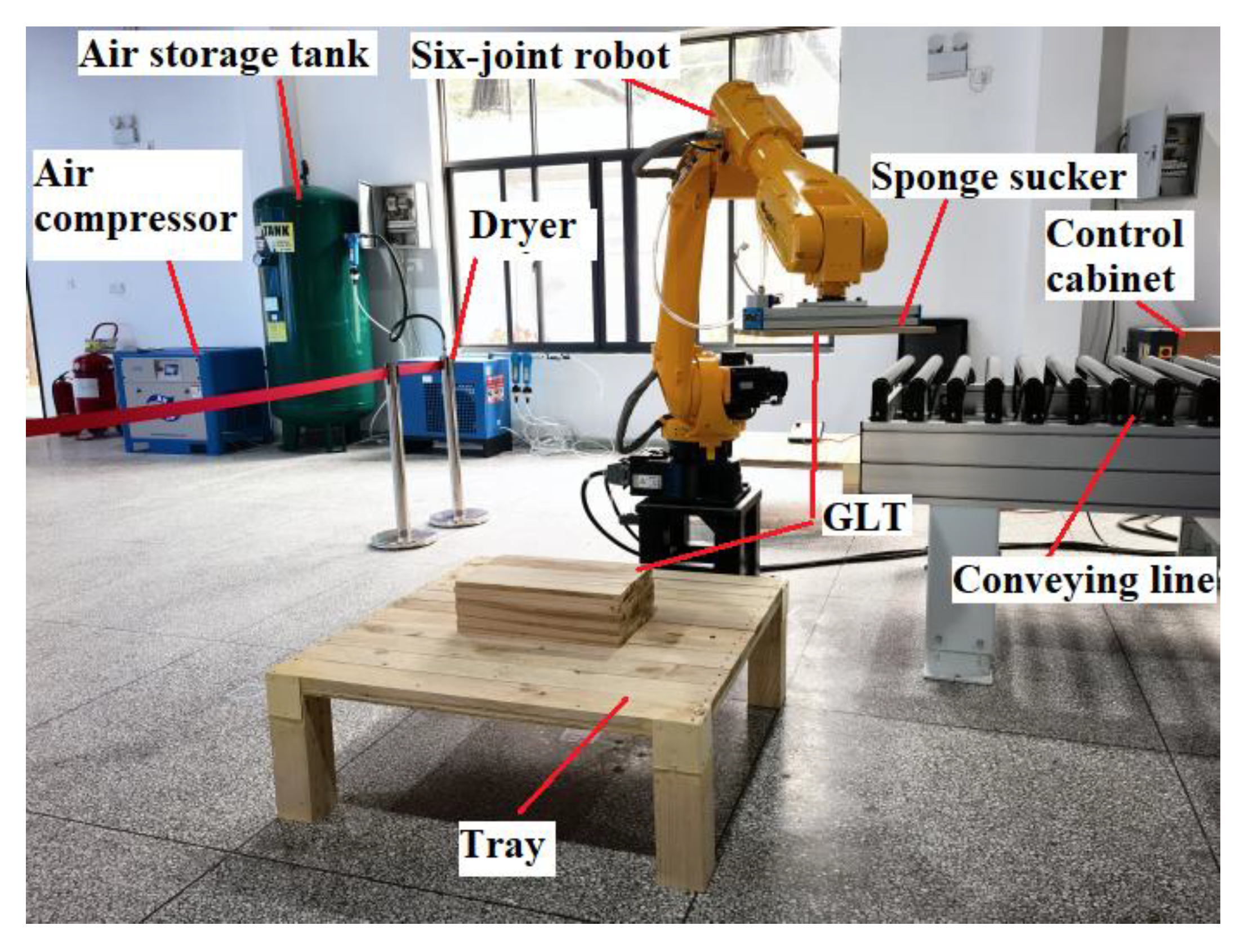
Aiming to solve the problems of low automation levels of loading and unloading, palletizing and high labor cost in the process of wood structure production, this paper adopted a six-axis robot with a sponge sucker as the grasping actuator to carry out research on the intelligent, automatic loading and unloading of GLT, which can improve the intelligent manufacturing level of wood structures. The research conclusions are as follows:
(2)
According to the Craig reference coordinate system establishment agreement, the robot link coordinate system was established, the D-H parameters of each link were determined according to the Denavit–Hartenberg method, and the mathematical model was established. The forward kinematics of the robot was deduced and solved. The kinematics model of GLT loading and unloading robot was built using Matlab robots, and the simulation results were verified using simulation technology, proving the motion analysis’s correctness.
(3)
In the Matlab environment, the working space of robot was simulated and analyzed via the Monte Carlo method, and the scope of robot working space was determined. The analysis results show that the robot has a flexible structure and a wide range of working space, which can meet the requirements for palletizing and loading GLT and provide a theoretical basis for the robot’s automatic loading and unloading operation trajectory planning and automatic control research.
(4)
The simulation results show that the method of high-order quintic and sixth-order polynomial curve interpolation can be used to plan the trajectory of wood structure parts in the process of a loading and unloading operation under the two conditions of staying and not staying. It can ensure the tracking accuracy of the trajectory. At the same time, it can also provide continuous and stable movement without impacts, large vibrations or other adverse conditions.
A verification test was carried out on the test platform of the palletizing robot for laminated material loading and unloading. The results show that the kinematics model of the robot for structural part loading and unloading was correct, and the analysis method was feasible. The robot working space drawn using the Monte Carlo method can intuitively and effectively analyze the robot’s working range.
(5)
The robot’s automatic loading and unloading operation trajectory planning provides data support and parameter basis for the automatic control and program design of the loading, unloading and palletizing robot.
(6)
This palletizing robot is only suitable for loading and unloading small-sized GLT. Large-sized laminated materials require a truss-type manipulator for loading, unloading and palletizing operations.
(7)
Further research will be carried out in loading and unloading experiments according to the results regarding the robot’s automatic loading and unloading operation trajectory planning to prove it is correct and effective.

Author Contributions

Conceptualization, R.G. and W.Z.; methodology, R.G.; software, R.G. and G.W.; validation, X.W. and G.W.; formal analysis, R.G.; investigation, G.W. and X.W.; data curation, W.Z. and G.W.; writing—original draft preparation, R.G.; writing—review and editing, R.G. and W.Z.; supervision, X.W.; project administration, W.Z.; funding acquisition, W.Z. All authors have read and agreed to the published version of the manuscript.

Funding

This work was supported by the Program of Forestry Science and Technology Promotion Project of the State Forestry and Grassland Administration of China (Grant No. [2019]35); National Natural Science Foundation of China (CN) (Grant No. 31670721). The central government guides local scientific and technological development projects (CN) (Grant No. 2022L3063) and Key project of basic research funds for public welfare research institutes at the central level (Grant No. CAFYBB2018ZB011); Forestry Science and Technology Project of Fujian province (Grant Nos. 2021FKJ01 and 2021FKJ12); Fujian Provincial Science and Technology Plan Project (Grant No. 2022R1010005).

Conflicts of Interest

The authors declare no conflict of interest.

References

  1. Zaman, A.; Chan, Y.-Q.; Jonescu, E.; Stewart, I. Critical Challenges and Potential for Widespread Adoption of Mass Timber Construction in Australia—An Analysis of Industry Perceptions. Buildings 2022, 12, 1405. [Google Scholar] [CrossRef]
  2. Xu, B.-H.; Bouchair, A.; Taazount, M.; Racher, P. Numerical simulation of embedding strength of glued laminated timber for dowel-type fasteners. J. Wood Sci. 2013, 59, 17–23. [Google Scholar] [CrossRef]
  3. Ren, T.; Luo, T.; Li, S.; Xing, L.; Xiang, S. Review on R&D task integrated management of intelligent manufacturing equipment. Neural Comput. Applic. 2022, 34, 5813–5837. [Google Scholar] [CrossRef]
  4. Mirski, R.; Dziurka, D.; Chuda-Kowalska, M.; Kawalerczyk, J.; Kuliński, M.; Łabęda, K. The Usefulness of Pine Timber (Pinus sylvestris L.) for the Production of Structural Elements. Part II: Strength Properties of Glued Laminated Timber. Materials 2020, 13, 4029. [Google Scholar] [CrossRef]
  5. Pervaiz, S.; Kannan, S.; Subramaniam, A. Optimization of Cutting Process Parameters in Inclined Drilling of Inconel 718 Using Finite Element Method and Taguchi Analysis. Materials 2020, 13, 3995. [Google Scholar] [CrossRef]
  6. Fonseca, F.G.; Anca-Couce, A.; Funke, A.; Dahmen, N. Challenges in Kinetic Parameter Determination for Wheat Straw Pyrolysis. Energies 2022, 15, 7240. [Google Scholar] [CrossRef]
  7. Stolze, H.; Gurnik, M.; Koddenberg, T.; Kröger, J.; Köhler, R.; Viöl, W.; Militz, H. Non-Destructive Evaluation of the Cutting Surface of Hardwood Finger Joints. Sensors 2022, 22, 3855. [Google Scholar] [CrossRef]
  8. Zhang, Y.; Bi, Q.; Yu, L.; Wang, Y. Online adaptive measurement and adjustment for flexible part during high precision drilling process. Int. J. Adv. Manuf. Technol. 2017, 89, 3579–3599. [Google Scholar] [CrossRef]
  9. Zhang, Z.; Zhu, Z.; Zhang, J.; Wang, J. Construction of intelligent integrated model framework for the workshop manufacturing system via digital twin. Int. J. Adv. Manuf. Technol. 2022, 118, 3119–3132. [Google Scholar] [CrossRef]
  10. Akter, S.T.; Bader, T.K. Experimental assessment of failure criteria for the interaction of normal stress perpendicular to the grain with rolling shear stress in Norway spruce clear wood. Eur. J. Wood Prod. 2020, 78, 1105–1123. [Google Scholar] [CrossRef]
  11. Zhang, Y.C.; Yang, C.Z.; Baker, C.; Chen, M.; Zou, X.; Dai, W.L. Effects of expanding zone parameters of vacuum dust suction mouth on flow simulation results. J. Cent. South Univ. 2014, 21, 2547–2552. [Google Scholar] [CrossRef]
  12. Daichin; Lee, S.J. Experimental analysis of flow fields inside intake heads of a vacuum cleaner. J. Mech. Sci. Technol. 2015, 19, 894–904. [Google Scholar] [CrossRef]
  13. Wu, J.; Liu, Y.; Zhao, J.; Zang, X.; Guan, Y. Research on Theory and a Performance Analysis of an Innovative Rehabilitation Robot. Sensors 2022, 22, 3929. [Google Scholar] [CrossRef]
  14. Sun, T.; Yang, S.-F.; Huang, T.; Dai, J.S. A Finite and Instantaneous Screw Based Approach for Topology Design and Kinematic Analysis of 5-Axis Parallel Kinematic Machines. Chin. J. Mech. Eng. 2018, 31, 44. [Google Scholar] [CrossRef] [Green Version]
  15. Klug, C.; Schmalstieg, D.; Gloor, T.; Arth, C. A Complete Workflow for Automatic Forward Kinematics Model Extraction of Robotic Total Stations Using the Denavit-Hartenberg Convention. J. Intell. Robot. Syst. 2019, 95, 311–329. [Google Scholar] [CrossRef] [Green Version]
  16. Sadjadian, H.; Taghirad, H.D. Comparison of Different Methods for Computing the Forward Kinematics of a Redundant Parallel Manipulator. J. Intell. Robot. Syst. 2005, 44, 225–246. [Google Scholar] [CrossRef]
  17. Wang, Y.; Yu, J.; Pei, X. Fast forward kinematics algorithm for real-time and high-precision control of the 3-RPS parallel mechanism. Front. Mech. Eng. 2018, 13, 368–375. [Google Scholar] [CrossRef]
  18. Wang, K.; Li, J.; Shen, H.; You, J.; Yang, T. Inverse Dynamics of A 3-DOF Parallel Mechanism Based on Analytical Forward Kinematics. Chin. J. Mech. Eng. 2022, 35, 119. [Google Scholar] [CrossRef]
  19. Yang, C.-F.; Zheng, S.-T.; Jin, J.; Zhu, S.-B.; Han, J.-W. Forward kinematics analysis of parallel manipulator using modified global Newton-Raphson method. J. Cent. South Univ. Technol. 2010, 17, 1264–1270. [Google Scholar] [CrossRef]
  20. Fabietti, M.; Mahmud, M.; Lotfi, A.; Kaiser, M.S.; Averna, A.; Guggenmos, D.J.; Nudo, R.J.; Chiappalone, M.; Chen, J. SANTIA: A Matlab-based open-source toolbox for artifact detection and removal from extracellular neuronal signals. Brain Inf. 2021, 8, 14. [Google Scholar] [CrossRef]
  21. Hadi Barhaghtalab, M.; Meigoli, V.; Golbahar Haghighi, M.R.; Nayeri, S.A.; Ebrahimi, A. Dynamic analysis, simulation, and control of a 6-DOF IRB-120 robot manipulator using sliding mode control and boundary layer method. J. Cent. South Univ. 2018, 25, 2219–2244. [Google Scholar] [CrossRef]
  22. Mackay, A.K.; Riazuelo, L.; Montano, L. RL-DOVS: Reinforcement Learning for Autonomous Robot Navigation in Dynamic Environments. Sensors 2022, 22, 3847. [Google Scholar] [CrossRef] [PubMed]
  23. Kulakov, F.M. Methods of Supervisory Remote Control over Space Robots. J. Comput. Syst. Sci. Int. 2018, 57, 822–839. [Google Scholar] [CrossRef]
  24. Lapshin, V.V. On the Workspace of a Free-Floating Space Robot. J. Comput. Syst. Sci. Int. 2018, 57, 149–156. [Google Scholar] [CrossRef]
  25. Dias, T.; Oliveira, R.; Saraiva, P.M.; Reis, M.S. Linear and Non-Linear Soft Sensors for Predicting the Research Octane Number (RON) through Integrated Synchronization, Resolution Selection and Modelling. Sensors 2022, 22, 3734. [Google Scholar] [CrossRef]
  26. Li, L.; Liu, Z.; Jin, J.; Xue, J. A modified method for the prediction of Monte Carlo simulation based on the similarity of random field instances. Geomech. Geophys. Geo-Energy Geo-Resour. 2021, 7, 37. [Google Scholar] [CrossRef]
  27. Subad, R.A.S.I.; Saikot, M.M.H.; Park, K. Soft Multi-Directional Force Sensor for Underwater Robotic Application. Sensors 2022, 22, 3850. [Google Scholar] [CrossRef]
  28. Glogowski, P.; Böhmer, A.; Hypki, A.; Kuhlenkötter, B. Robot Speed Adaption in Multiple Trajectory Planning and Integration in a Simulation Tool for Human-Robot Interaction. J. Intell. Robot. Syst. 2021, 102, 25. [Google Scholar] [CrossRef]
  29. Park, S.O.; Lee, M.C.; Kim, J. Trajectory Planning with Collision Avoidance for Redundant Robots Using Jacobian and Artificial Potential Field-based Real-time Inverse Kinematics. Int. J. Control Autom. Syst. 2020, 18, 2095–2107. [Google Scholar] [CrossRef]
  30. Luo, L.-P.; Yuan, C.; Yan, R.-J.; Yuan, Q.; Wu, J.; Shin, K.-S.; Han, C.-S. Trajectory planning for energy minimization of industry robotic manipulators using the Lagrange interpolation method. Int. J. Precis. Eng. Manuf. 2015, 16, 911–917. [Google Scholar] [CrossRef]
  31. Farouki, R.T. Quaternion and Hopf map characterizations for the existence of rational rotation-minimizing frames on quintic space curves. Adv. Comput. Math. 2010, 33, 331–348. [Google Scholar] [CrossRef] [Green Version]
Figure 1. Schematic diagram of palletizing robot. 1. Base; 2. waist link rod; 3. large arm link rod; 4. elbow link rod; 5. small arm link rod; 6. wrist link rod; 7. rotary flange; 8. end actuator.
Buildings 13 00966 g001
Figure 2. D-H coordinate system. (Notes: The distance between these two normals was di.θi, which is the angle between two connecting rods; di is the distance between two links; ai is the length of the connecting rod; and αi is the torsion angle of the connecting rod.)
Buildings 13 00966 g002
Figure 3. Three-dimensional model of robot.
Buildings 13 00966 g003
Figure 4. Cloud image of robot. (a) Three-dimensional graph, (b) X-Y diagram, (c) X-Z diagram, (d) Y-Z diagram.
Buildings 13 00966 g004
Figure 5. The path planning of loading operation: (a) graphic model, (b) Y-Z diagrammatic sketch.
Buildings 13 00966 g005
Figure 6. The track curve of loading.
Buildings 13 00966 g006
Figure 7. The displacement, velocity and acceleration curve of each joint.
Buildings 13 00966 g007
Figure 8. The track curve of loading.
Buildings 13 00966 g008
Figure 9. The curve of displacement, velocity and acceleration of each joint.
Buildings 13 00966 g009
Figure 10. Robot experiment site.
Buildings 13 00966 g010
Table 1. Improved D-H parameter table.
Jointθi/raddi/mαi−1/radai−1/mJoint Rotation Range/rad
100pi0−178/pi~178/pi
2−pi/20pi/2149.078−98/pi~158/pi
3000790.385−178/pi~78/pi
4pi−860.711pi/2150.305−400/pi~400/pi
5pi0pi/20−120/pi~120/pi
6pi0pi/20500/pi~500/pi
Table 2. The posture teaching results and simulation comparison results of the end effector.
Group NumberMethodθ1θ2θ3θ4θ5θ6Result
X/mmY/mmZ/mmRPY
1equation1530456090160783.71−336.47323.58100.30−43.6890.22
simulation783.71−336.47323.58100.30−43.6890.22
2equation9060402515300−15.43−775.88−157.17−156.35−6.28125.75
simulation−15.43−775.88−157.17−156.35−6.28125.75
3equation0107−11032055101842.0374.28329.72−138.5737.27−12.42
simulation1842.0374.28329.72−138.5737.27−12.42
Table 3. Results of inverse kinematics simulation.
Group NumberThe End Effector Sits in the Base Coordinate FrameResult
X/mmY/mmZ/mmRPYθ1θ2θ3θ4θ5θ6
1783.71−336.47323.58100.30−43.6890.221530456090200
2−14.43−775.83−157.17−156.35−6.28125.759060402515300
31842.0374.28329.72−138.5737.27−12.420107−1103205510
Table 4. Coordinates of the path’s key points.
Key PointsEnd-Effector Coordinates in the Base Coordinate SystemJoint Coordinate
X/mmY/mmZ/mmRPYθ1θ2θ3θ4θ5θ6
Target point A0−1280559001809053.7511.77024.480
Way point B640−1108.57066001806023.887.89058.230
Target point C1280061600180026.5910.52052.890
Table 5. The results of posture teaching and the end effector’s simulation comparison.
Group NumberMethodθ1θ2θ3θ4θ5θ6Result
X/mmY/mmZ/mmRPY
1Test verification0−13.960082.840808.2501438.84021.13180
Simulation808.2601438.78021.12180
2Test verification145.19−39.48−39.409.3090.46−19.69150.00132.041905.55130.60−62.38115.30
Simulation150.02132.071905.46130.60−62.38115.31
3Test verification−171.3336.61−39.409.3090.46−19.69−1458.19245.481137.23−151.30−0.88−170.46
Simulation−1458.12245.401137.198−151.30−0.87−170.46
Disclaimer/Publisher’s Note: The statements, opinions and data contained in all publications are solely those of the individual author(s) and contributor(s) and not of MDPI and/or the editor(s). MDPI and/or the editor(s) disclaim responsibility for any injury to people or property resulting from any ideas, methods, instructions or products referred to in the content.

