
Classification of Multiaxial Behaviour of Fine-Grained Concrete for the Calibration of a Microplane Plasticity Model


Abstract
:1. Introduction
2. Microplane Drucker–Prager Cap Plasticity
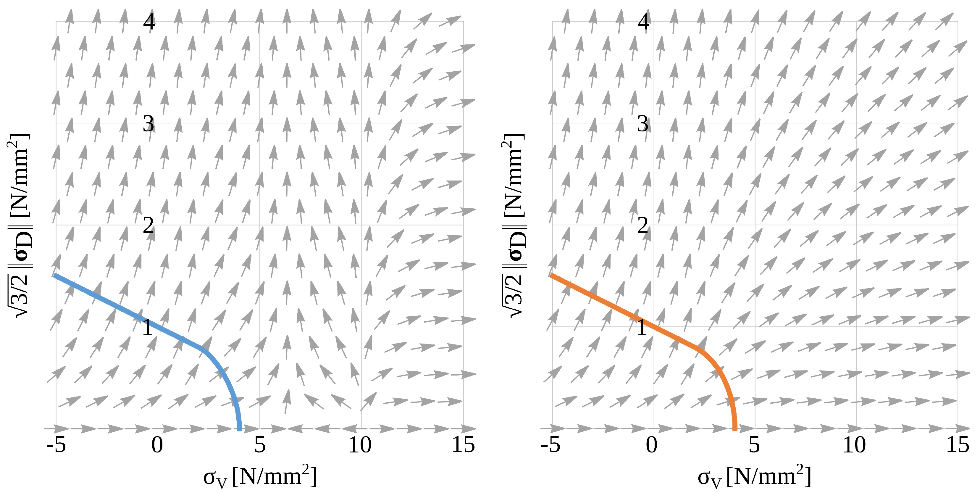
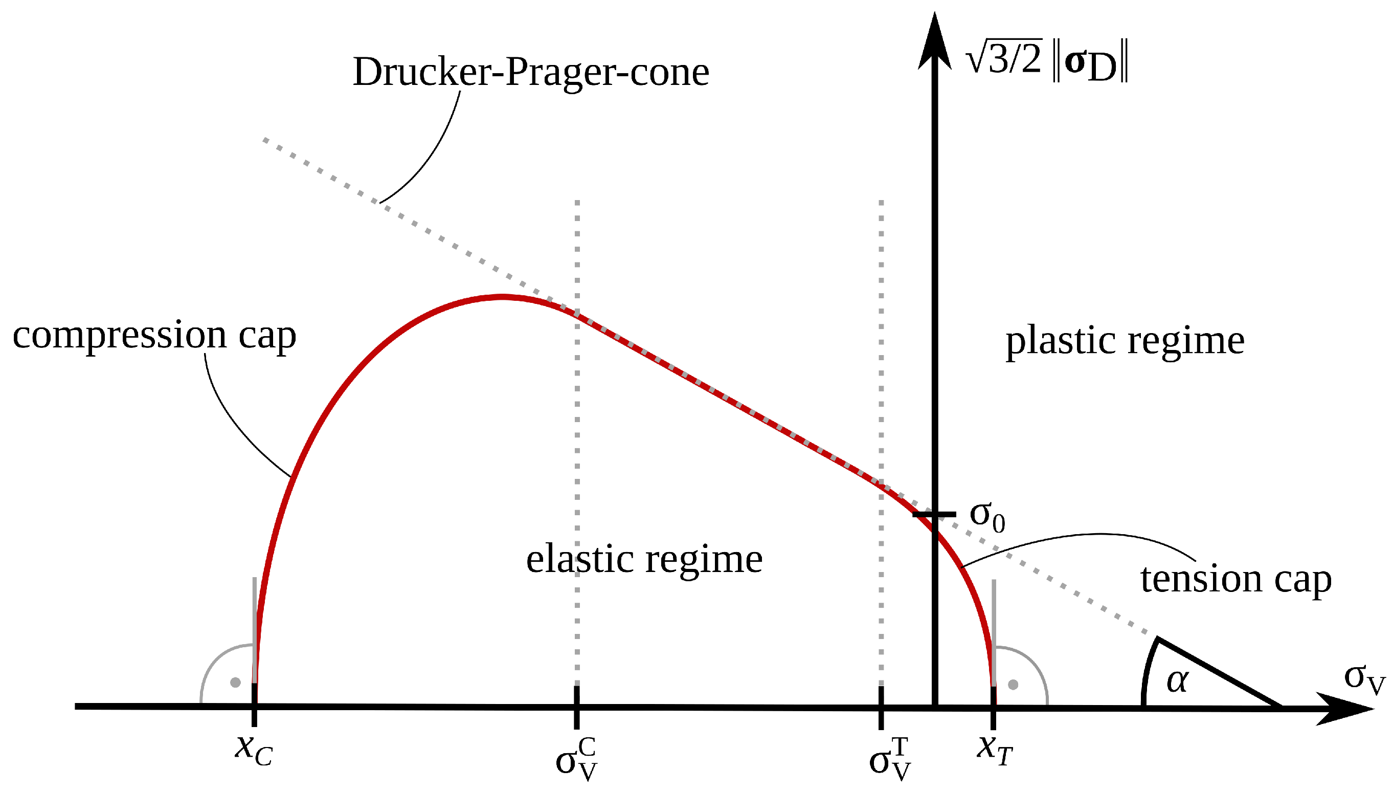
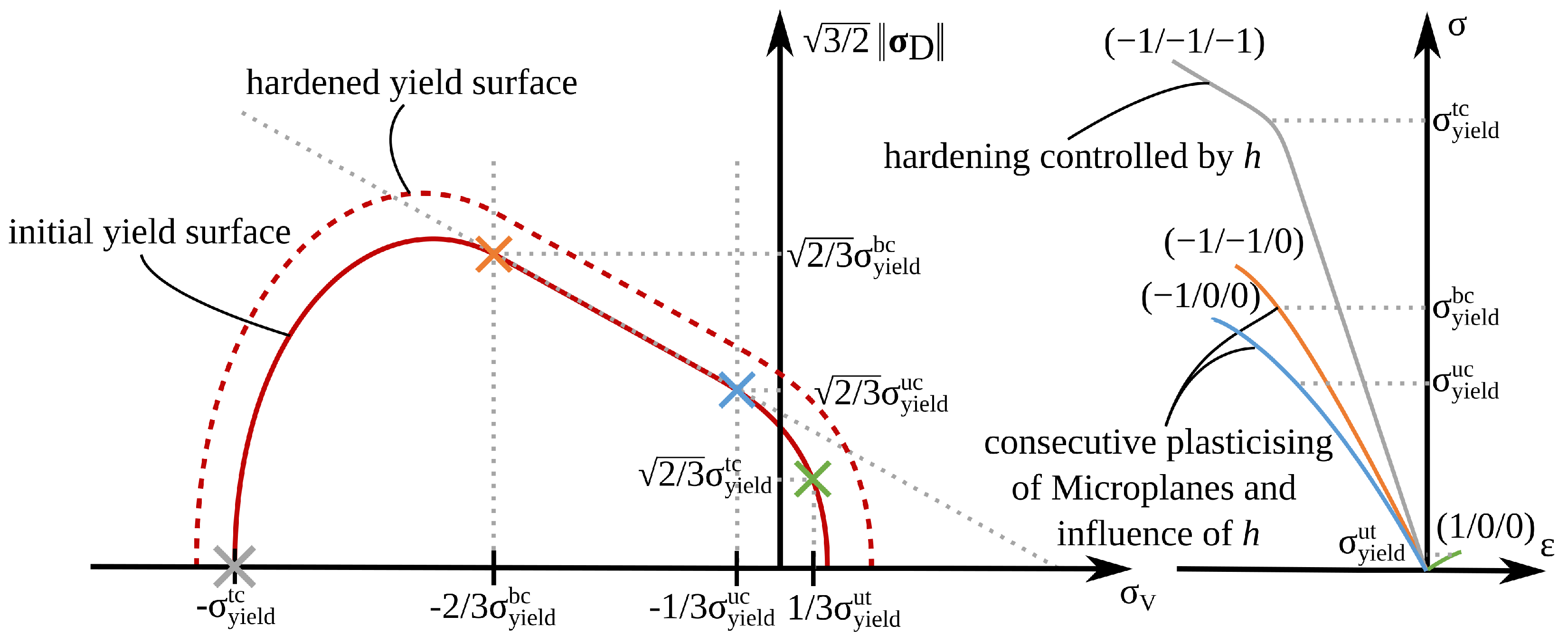
2.1. Formulation of the Material Model
2.2. A Discussion of Material Parameter Fitting for the Numerical Model
3. Experimental Investigations
3.1. Background
3.2. Experimental Methodology
3.3. Material
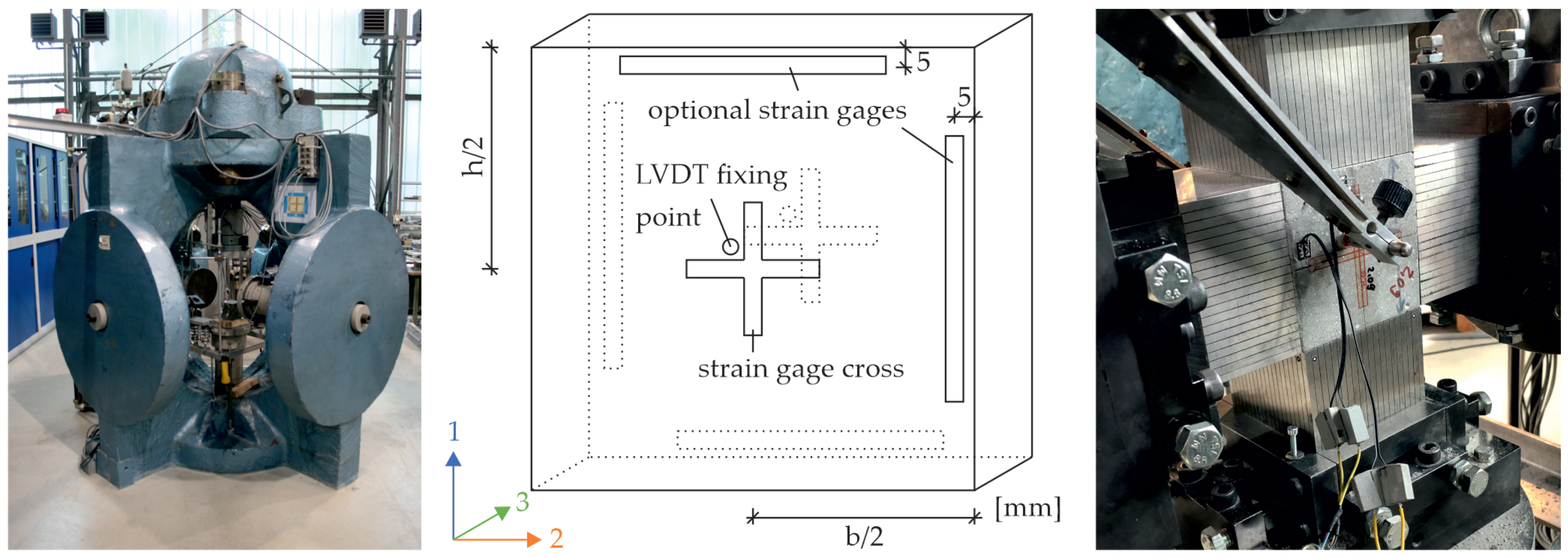
3.4. Test Setup
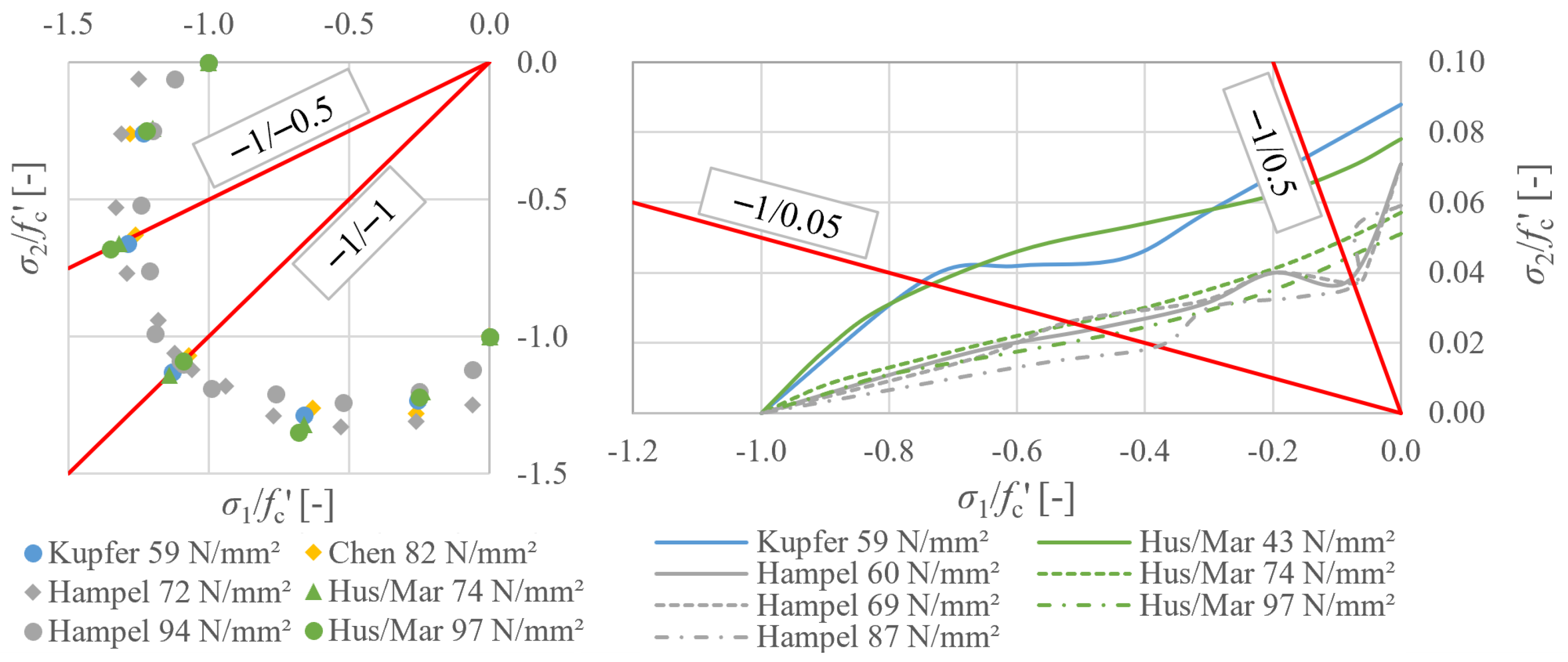
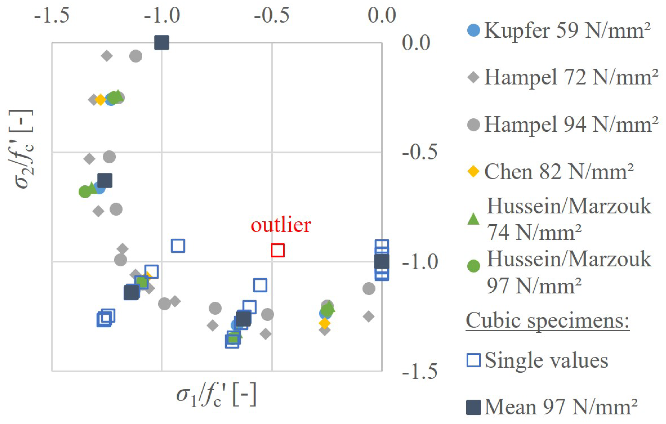
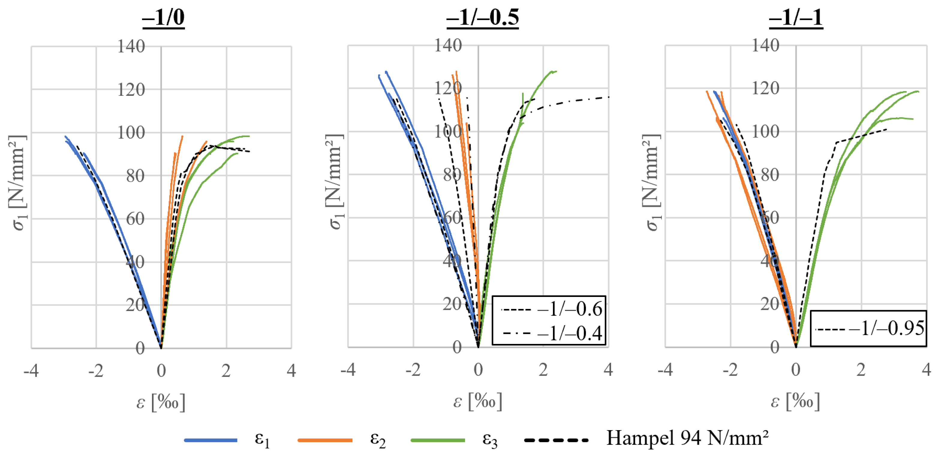
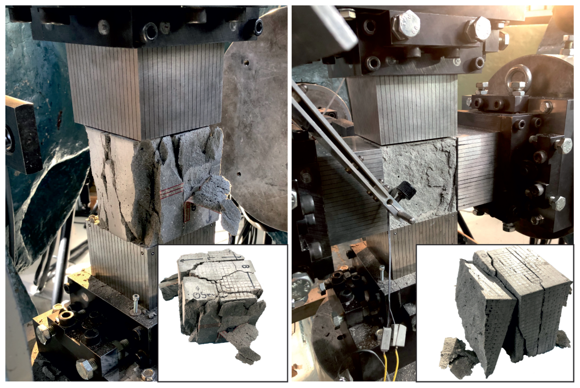
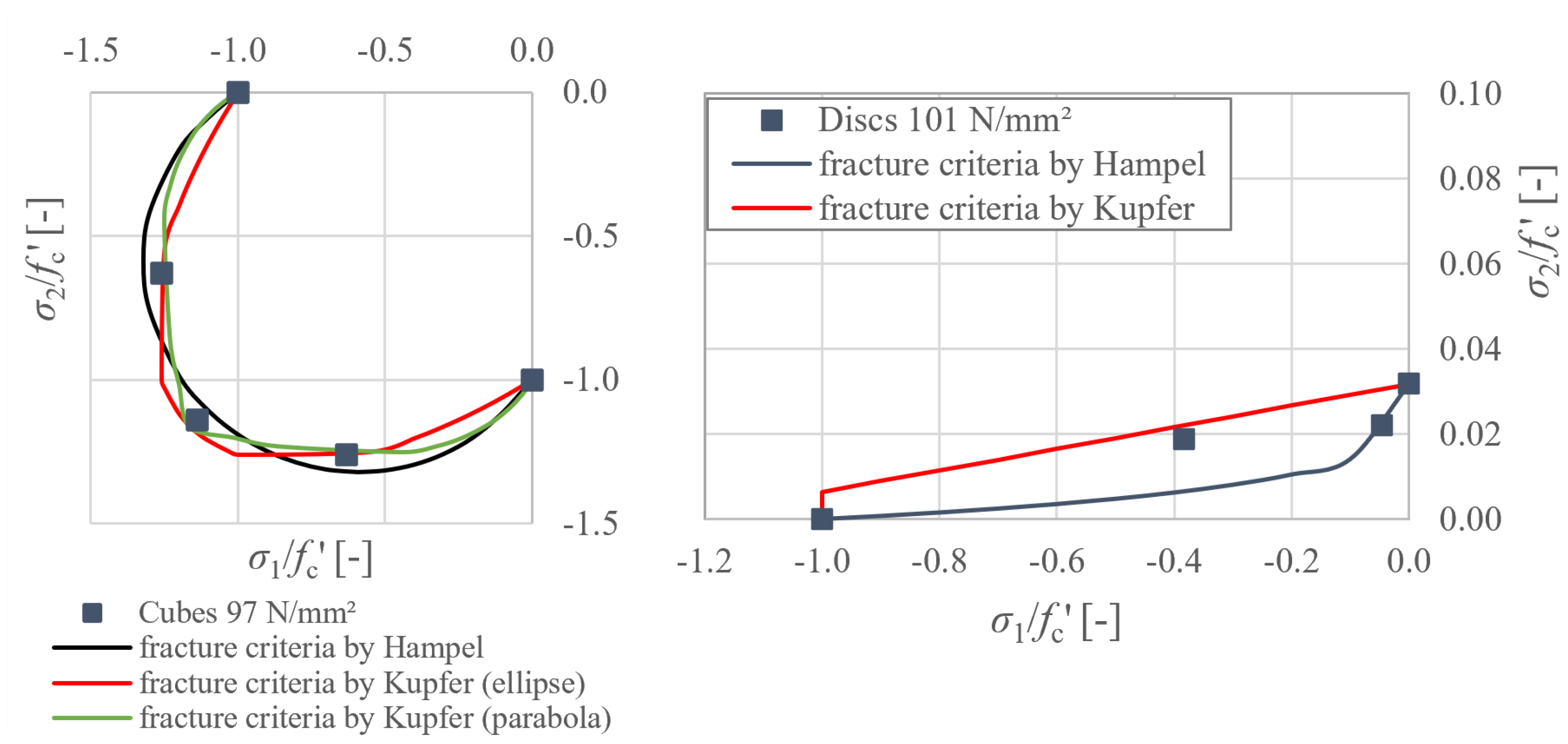
3.5. Biaxial Compressive Strength
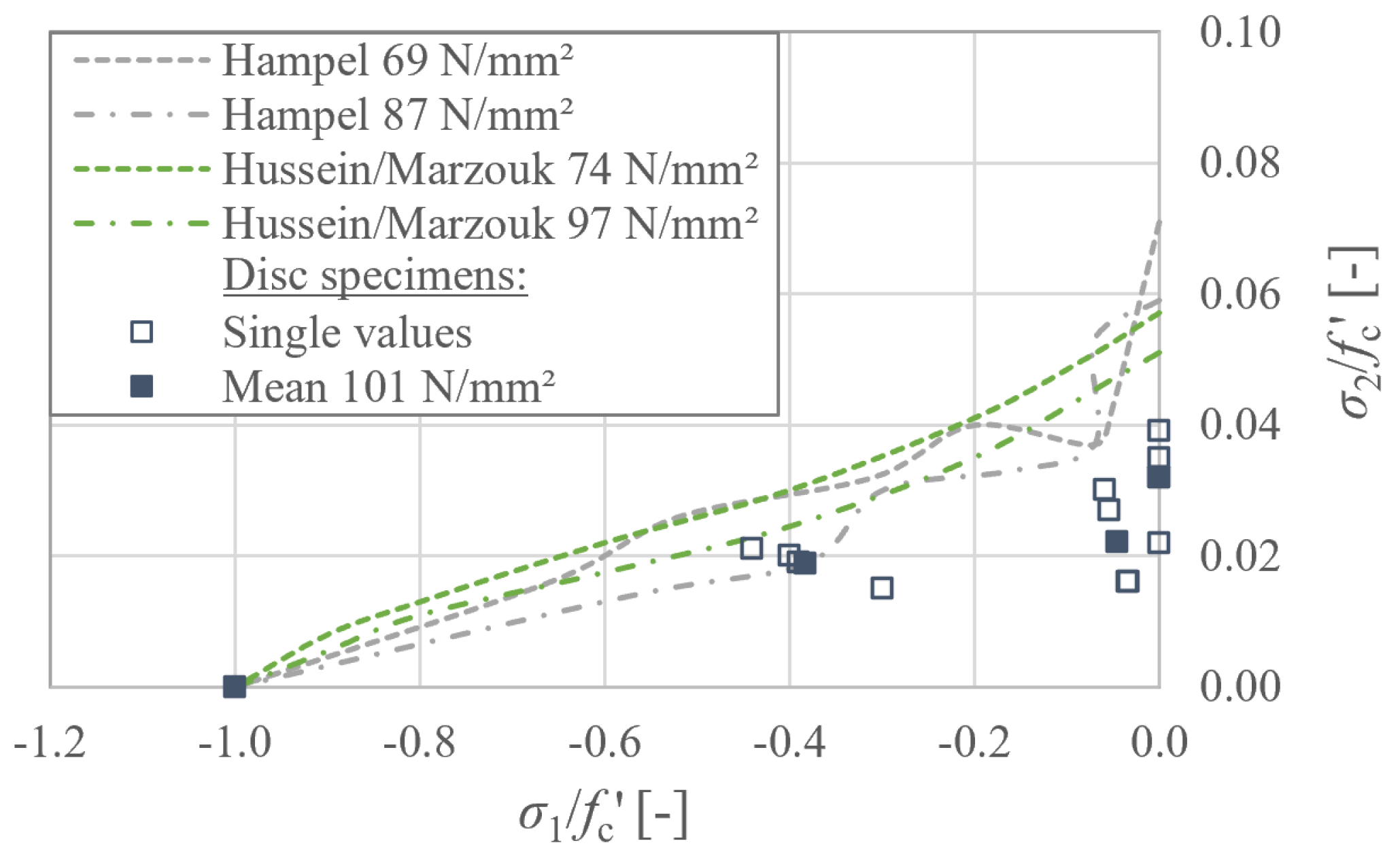
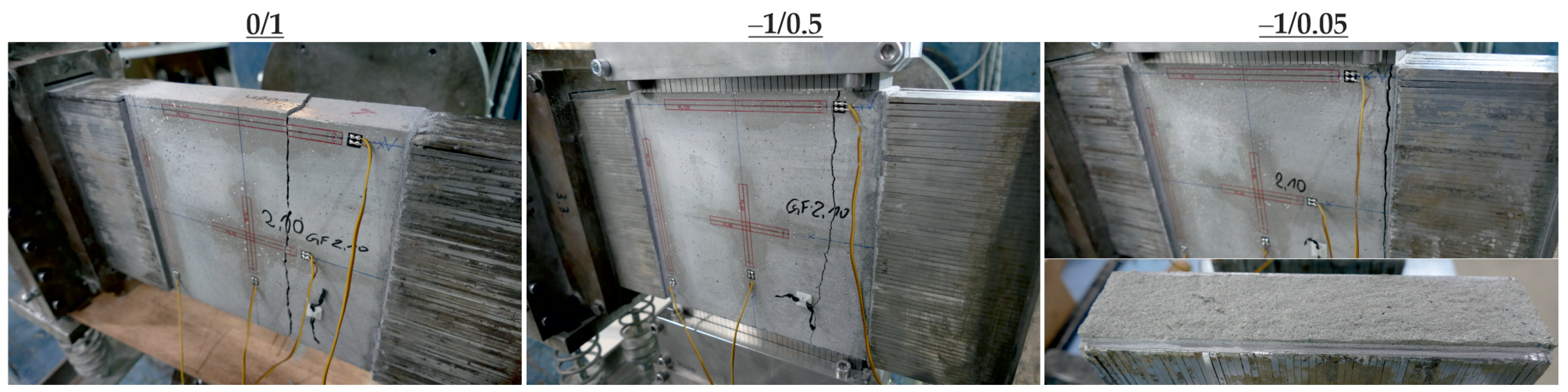
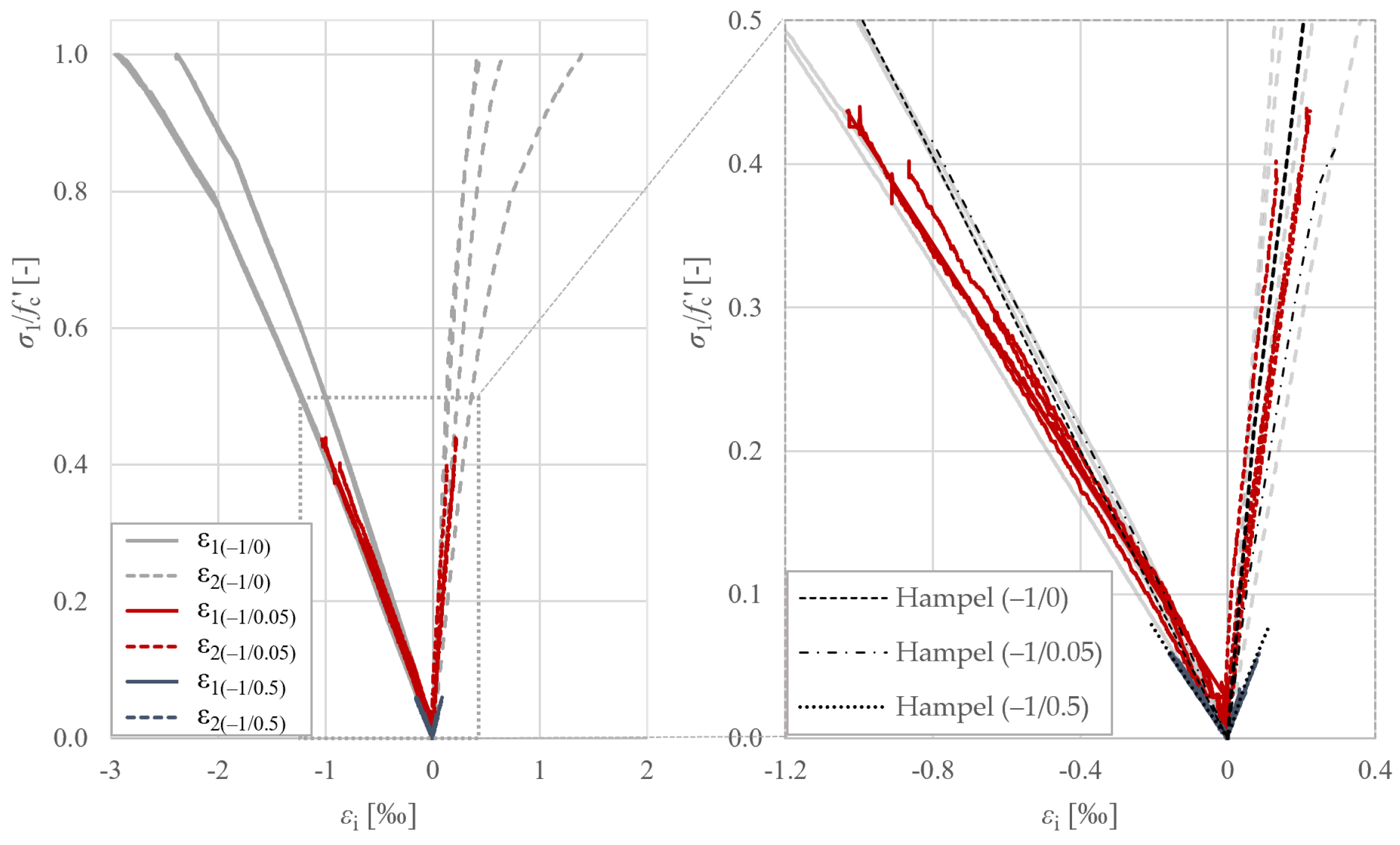
3.6. Compressive Strength with Transversal Tensile Stress
4. Discussion
4.1. Experimental Results
4.2. Parameter Fitting
5. Conclusions
Author Contributions
Funding
Data Availability Statement
Conflicts of Interest
References
- Triantafillou, T.C. Textile Fibre Composites in Civil Engineering; Woodhead Publishing: Sawston, UK, 2016. [Google Scholar] [CrossRef]
- Spelter, A.; Bergmann, S.; Bielak, J.; Hegger, J. Long-Term Durability of Carbon-Reinforced Concrete: An Overview and Experimental Investigations. Appl. Sci. 2019, 9, 1651. [Google Scholar] [CrossRef]
- Valeri, P.; Guaita, P.; Baur, R.; Fernández Ruiz, M.; Fernández-Ordóñez, D.; Muttoni, A. Textile reinforced concrete for sustainable structures: Future perspectives and application to a prototype pavilion. Struct. Concr. 2020, 21, 2251–2267. [Google Scholar] [CrossRef]
- Giese, J.; Beckmann, B.; Schladitz, F.; Marx, S.; Curbach, M. Effect of Load Eccentricity on CRC Structures with Different Slenderness Ratios Subjected to Axial Compression. Buildings 2023, 13, 2489. [Google Scholar] [CrossRef]
- Beckmann, B.; Bielak, J.; Bosbach, S.; Scheerer, S.; Schmidt, C.; Hegger, J.; Curbach, M. Collaborative research on carbon reinforced concrete structures in the CRC/TRR 280 project. Civ. Eng. Des. 2021, 3, 99–109. [Google Scholar] [CrossRef]
- Lieboldt, M. Feinbetonmatrix für Textilbeton: Anforderungen—baupraktische Adaption—Eigenschaften. Beton- und Stahlbetonbau 2015, 110, 22–28. [Google Scholar] [CrossRef]
- Brockmann, T. Mechanical and Fracture Mechanical Properties of Fine Grained Concrete for Textile Reinforced Composites. Ph.D. Dissertation, RWTH Aachen University, Aachen, Germany, 2006. [Google Scholar]
- Bochmann, J.; Jesse, F.; Curbach, M. Experimental Determination of the Stress-Strain Relation of Fine Grained Concrete under Compression. In Proceedings of 11th HPC and 2nd CIC Conference, Tromso, Norway, 6–7 March 2017; Paper No. 6; Justnes, H., Martius-Hammer, T.A., Eds.; Norwegian Concrete Association/Tekna: Oslo, Norway, 2017. [Google Scholar]
- Bochmann, J. Carbonbeton unter Einaxialer Druckbeanspruchung. Ph.D. Dissertation, Technische Universität Dresden, Dresden, Germany, 2019. [Google Scholar]
- Bosbach, S.; Bielak, J.; Schmidt, C.; Hegger, J.; Claßen, M. Influence of Transverse Tension on the Compressive Strength of Carbon Reinforced Concrete. In Proceedings of the 11th International Conference on Fiber-Reinforced Polymer (FRP) Composites in Civil Engineering (CICE 2023), Rio de Janeiro, Brazil, 24–26 July 2023. Paper 328. [Google Scholar] [CrossRef]
- Kupfer, H. Das Verhalten des Betons unter Zweiachsiger Beanspruchung. Wiss. Z. Tech. Univ. Dresd. 1968, 17, 1515–1518. [Google Scholar]
- Kupfer, H. Das Verhalten des Betons unter Mehrachsiger Kurzzeitbelastung unter Besonderer Berücksichtigung der Zweiachsigen Beanspruchung. In Schriftreihe des DAfStb; Deutscher Ausschuss für Stahlbeton: Berlin, Germany, 1973; Volume 229. [Google Scholar]
- Chen, R.L. Behavior of High-Strength Concrete in Biaxial Compression. Ph.D. Dissertation, University of Texas, Austin, TX, USA, 1984. [Google Scholar]
- Hussein, A.; Marzouk, H. Behavior of High-Strength Concrete under Biaxial Loading. ACI Mater. J. 2000, 97, 27–36. [Google Scholar]
- Hampel, T. Experimentelle Analyse des Tragverhaltens von Hochleistungsbeton unter Mehraxialer Beanspruchung. Ph.D. Dissertation, TU Dresden, Dresden, Germany, 2006. [Google Scholar]
- Speck, K. Beton unter Mehraxialer Belastung—Ein Materialgesetz für Hochleistungsbetone unter Kurzzeitbelastung. Ph.D. Dissertation, TU Dresden, Dresden, Germany, 2007. [Google Scholar]
- Hampel, T.; Speck, K.; Scheerer, S.; Ritter, R.; Curbach, M. High-Performance Concrete under Biaxial and Triaxial Loads. J. Eng. Mech. 2009, 135, 1274–1280. [Google Scholar] [CrossRef]
- Bazant, Z.P.; Oh, B.H. Microplane model for fracture analysis of concrete structures. In Proceedings of the Symposium on the Interaction of Non-Nuclear Munitions with Structures, Colorado Springs, CO, USA, 10–13 May 1983; pp. 49–53. [Google Scholar]
- Zreid, I.; Kaliske, M. A gradient enhanced plasticity–damage microplane model for concrete. Comput. Mech. 2018, 62, 1239–1257. [Google Scholar] [CrossRef]
- Fuchs, E.; Kaliske, M. A gradient enhanced viscoplasticity-damage microplane model for concrete at static and transient loading. In Proceedings of the 10th International Conference on Fracture Mechanics of Concrete and Concrete Structures, Bayonne, France, 23–26 June 2019; pp. 23–26. [Google Scholar] [CrossRef]
- Bazant, Z.P.; Planas, J. Fracture and Size Effect in Concrete and Other Quasibrittle Materials; Routledge: New York, NY, USA, 2019; (print version published 1998). [Google Scholar] [CrossRef]
- Carol, I.; Jirásek, M.; Bažant, Z. A thermodynamically consistent approach to microplane theory. Part I. Free energy and consistent microplane stresses. Int. J. Solids Struct. 2001, 38, 2921–2931. [Google Scholar] [CrossRef]
- Bažant, P.; Oh, B. Efficient numerical integration on the surface of a sphere. ZAMM-J. Appl. Math. Mech. Für Angew. Math. Und Mech. 1986, 66, 37–49. [Google Scholar] [CrossRef]
- Zreid, I.; Kaliske, M. An implicit gradient formulation for microplane Drucker-Prager plasticity. Int. J. Plast. 2016, 83, 252–272. [Google Scholar] [CrossRef]
- Wriggers, P. Nonlinear Finite Element Methods; Springer Science & Business Media: Berlin/Heidelberg, Germany, 2008. [Google Scholar] [CrossRef]
- Leukart, M.; Ramm, E. Identification and interpretation of microplane material laws. J. Eng. Mech. 2006, 132, 295–305. [Google Scholar] [CrossRef]
- Qinami, A.; Pandolfi, A.; Kaliske, M. Variational eigenerosion for rate-dependent plasticity in concrete modeling at small strain. Int. J. Numer. Methods Eng. 2020, 121, 1388–1409. [Google Scholar] [CrossRef]
- Platen, J.; Zreid, I.; Kaliske, M. A nonlocal microplane approach to model textile reinforced concrete at finite deformations. Int. J. Solids Struct. 2023, 267, 112151. [Google Scholar] [CrossRef]
- Pagel Spezial-Beton GmbH & Co. KG. Datenblatt Pagel TF10 CARBOrefit® Textilfeinbeton; Pagel Spezial-Beton GmbH & Co. KG: Essen, Germany, 2022. [Google Scholar]
- Deutsches Institut für Bautechnik. CARBOrefit®—Verfahren zur Verstärkung von Stahlbeton mit Carbonbeton: Allgemeine Bauaufsichtliche Zulassung (abZ)/Allgemeine Bauartgenehmigung (aBG) Z-31.10-182; Deutsches Institut für Bautechnik: Berlin, Germany, 2021. [Google Scholar]
- DIN EN 206:2013+A2:2021; Concrete—Specification, Performance, Production and Conformity. Beuth-Verlag: Berlin, Germany, 2021.
- Frenzel, M.; Tietze, M.; Curbach, M. C3 Technology Demonstration House—CUBE: Design and Manufacturing of the Twisted Roof-Wall Construction. In Proceedings of the 6th fib International Congress, Oslo, Norway, 12–16 June 2022; pp. 2542–2550. [Google Scholar]
- Hering, M. Untersuchung von Mineralisch Gebundenen Verstärkungsschichten für Stahlbetonplatten gegen Impaktbeanspruchungen. Ph.D. Dissertation, Technische Universität Dresden, Dresden, Germany, 2020. [Google Scholar]
- DIN EN 196-1:2016; Methods of Testing Cement—Part 1: Determination of Strength. Beuth-Verlag: Berlin, Germany, 2016.
- Betz, P.; Marx, S.; Curbach, M. Einfluss von Querzugspannungen auf die Druckfestigkeit von Carbonbeton. Beton- und Stahlbetonbau 2023, 118, 524–533. [Google Scholar] [CrossRef]
- Bazant, Z.P. Size effect on structural strength: A review. Arch. Appl. Mech. 1999, 69, 703–725. [Google Scholar]
- Wosatko, A.; Winnicki, A.; Polak, M.A.; Pamin, J. Role of dilatancy angle in plasticity-based models of concrete. Arch. Civ. Mech. Eng. 2019, 19, 1268–1283. [Google Scholar] [CrossRef]
- Yu, T.; Teng, J.; Wong, Y.; Dong, S. Finite element modeling of confined concrete-I: Drucker–Prager type plasticity model. Eng. Struct. 2010, 32, 665–679. [Google Scholar] [CrossRef]


| Biaxial Compressive Loads | Compressive-Tensile Loads | |||||
|---|---|---|---|---|---|---|
| −1/0 | −1/−0.5 | −1/−1 | −1/0.05 | −1/0.5 | 0/1 | |
| Cubes | ||||||
| Batch 1 (tested after 28 days) | 4 | 4 | 4 | - | - | - |
| Batch 2 (tested after 43 days) | 4 | 4 | 4 | - | - | - |
| Discs | ||||||
| Batch 1 (tested after 56 days) | - | - | - | 2 | 2 | 2 |
| Batch 2 (tested after 63 days) | - | - | - | 2 | 2 | 2 |
| Compressive Strength [N/mm2] | Flexural Strength [N/mm2] | Young’s Modulus [N/mm2] | Poisson’s Ratio [-] | |
|---|---|---|---|---|
| Mean value prisms | 105.9 | 7.86 | 39,250 | - |
| (acc. to EN 196-1 [34]) | ||||
| Batch 1 | 102.9 | 6.9 | 38,750 | - |
| Batch 2 | 108.9 | 8.9 | 39,750 | - |
| Mean value cubes | 96.7 | - | 41,750 | 0.26 |
| (uniaxial compressive test) | ||||
| Batch 1 | 99.6 | - | 41,250 | 0.27 |
| Batch 2 | 93.7 | - | 42,250 | 0.24 |
| Compressive Strength [N/mm2] | Flexural Strength [N/mm2] | Tensile Strength [N/mm2] | Young’s Modulus [N/mm2] | Poisson’s Ratio [-] | |
|---|---|---|---|---|---|
| Mean value prisms | 100.7 | 7.76 | 4.06 | - | - |
| (acc. to EN 196-1 [34]) | - | - | - | - | - |
| Batch 1 | 101.5 | 6.84 | 3.79 | ||
| Batch 2 | 99.8 | 8.68 | 4.33 | ||
| Mean value discs | 87.6 | - | 2.79 | 35,000 | 0.26 |
| (uniaxial tensile tests) | (calc. 0.87 ) | (tensile) | (tensile) | ||
| Batch 1 | 88.3 (calc.) | - | 2.37 | ||
| Batch 2 | 86.8 (calc.) | - | 3.22 |
[-] | [N/mm2] | [N/mm2] | [N/mm2] | h [N/mm2] |
|---|---|---|---|---|
| 0.221 | 55.716 | −25 | −55.5 | 5000 |
Disclaimer/Publisher’s Note: The statements, opinions and data contained in all publications are solely those of the individual author(s) and contributor(s) and not of MDPI and/or the editor(s). MDPI and/or the editor(s) disclaim responsibility for any injury to people or property resulting from any ideas, methods, instructions or products referred to in the content. |
© 2023 by the authors. Licensee MDPI, Basel, Switzerland. This article is an open access article distributed under the terms and conditions of the Creative Commons Attribution (CC BY) license (https://creativecommons.org/licenses/by/4.0/).
Share and Cite
Betz, P.; Curosu, V.; Loehnert, S.; Marx, S.; Curbach, M. Classification of Multiaxial Behaviour of Fine-Grained Concrete for the Calibration of a Microplane Plasticity Model. Buildings 2023, 13, 2704. https://doi.org/10.3390/buildings13112704
Betz P, Curosu V, Loehnert S, Marx S, Curbach M. Classification of Multiaxial Behaviour of Fine-Grained Concrete for the Calibration of a Microplane Plasticity Model. Buildings. 2023; 13(11):2704. https://doi.org/10.3390/buildings13112704
Chicago/Turabian StyleBetz, Peter, Verena Curosu, Stefan Loehnert, Steffen Marx, and Manfred Curbach. 2023. "Classification of Multiaxial Behaviour of Fine-Grained Concrete for the Calibration of a Microplane Plasticity Model" Buildings 13, no. 11: 2704. https://doi.org/10.3390/buildings13112704