Damage Analysis and Quality Control of Carbon-Reinforced Concrete Beams Based on In Situ Computed Tomography Tests

Abstract

Carbon-reinforced concrete (CRC) is increasingly utilized in construction, due to its unique properties, such as corrosion resistance, high-tensile strength, and durability. Understanding its behavior under different loads is crucial to ensuring its safe and effective use in various construction applications. In this study, three-point bending tests were performed in combination with large-scale in situ computed tomography (CT). This paper presents the related three- and four-dimensional evaluation methods, with emphasis on crack width and quality control. The focus was on large CRC beams, with cross-sectional sizes of up to 80 mm by 160 mm. Such dimensions require extremely high energy during a CT scan. Therefore, a new experimental setup with energies of up to 8 MeV was used in this study. However, such high energies posed new challenges to the analysis methods. Therefore, two methods (digital volume correlation and grayscale profile analysis) for accurate crack width estimation were adapted and applied to the 3D reconstructions. In addition, a photogrammetric stereo image sequence was acquired and analyzed, using digital image correlation to cross-validate the results derived from the 3D crack width estimates. The 3D CT images also played a key role in the quality control measures, including the localization of the carbon-reinforcement and the assessment of porosity within the concrete structure.

1. Introduction

Concrete is currently the most important material for both residential and infrastructure construction. This versatile material has undergone a transformative evolution with the introduction of carbon-reinforced concrete (CRC), which is a composite material of fine-grained concrete and carbon reinforcement. As a result, it is resistant to corrosion—a key feature that has far-reaching implications for structural design.

The corrosion resistance provides a profound advantage, by allowing the concrete cover to be reduced to a minimum, since it results only from the bond requirements. In contrast to steel-reinforced concrete, the condition for compliance with durability can be omitted [1]. This feature alone transforms the possibilities of construction, allowing the creation of delicate, thin-walled members and structures, whether flat or curved. This innovation not only enhances the aesthetic potential of construction, but also takes a giant leap towards material conservation, which is instrumental in sustainable design strategies. In essence, CRC challenges the conventional notion of solid members and allows for entirely novel construction and design strategies [2].

However, due to the reduced cover of the concrete, the position of the reinforcement in the concrete has to be precise and the components have to be thoroughly tested and inspected. Computed tomography (CT) can essentially contribute to achieving this goal [3], as it is a non-destructive imaging method and a powerful tool for examining structural elements, including concrete beams [4]. Its capabilities extend beyond visual inspection: CT penetrates the internal structure and can track structural changes and, when performing in situ experiments, deformations over time [5]. This dual functionality serves quality control by enabling compositional analysis, crack detection, assessment of air void distribution, and localization of reinforcement within the concrete matrix [6]. In addition, changes in sequences of voxel datasets, such as those obtained by in situ tomography, can be analyzed using digital volume correlation (DVC) [7].

From the literature [8,9], micro-CT (µCT) has been the norm, limiting both power and sample size to a maximum cross-section of 75 × 75 mm${}^2$ and a maximum X-ray scan voltage of 210 keV. The usage of higher power is very rare, due to the challenges that are introduced. However, in [10] the authors investigated the maximum penetrable thickness of concrete, with respect to the tenth-value layer, using energies of up to 1332 keV. The tenth-value layer refers to a measurement that describes the thickness of a material required to reduce the intensity of an X-ray beam to one tenth (10%) of its original value. They have shown that the maximum thickness of concrete is still limited to 16 cm.

In the present study, these limitations were shattered, using a State-of-the-Art in situ experimental setup that allowed for sample cross-sections of up to 80 × 160 mm${}^2$ and energies of up to 8 MeV. The experiments were conducted at the Fraunhofer Development Center X-ray Technology (EZRT) in Fürth, Germany.

The experiments served as preliminary tests, to gain knowledge for a groundbreaking large-scale CT device (the tomography portal Gulliver), which is currently set up at Rheinland-Pfälzische Technische Universität Kaiserslautern-Landau (RPTU). During this study, the X-ray detector that will soon be integrated into Gulliver was used. When completed, the setup will provide X-ray energy of up to 9 MeV for the scan of concrete samples of up to 6 m in length and nearly 1 m in diameter during bending tests [11].

However, CT scans at such high energies introduce new challenges, with regard to the interpretability of the resulting volumetric images. For example, details related to fine elements of similar density are lost and strong noise is introduced [12].

In the context of this evolving landscape, this investigation takes center stage and presents in situ CT scans of three-point bending tests, performed on CRC beams. The primary objective of these experiments was to visualize and analyze the evolution of load-induced cracks in CRC beams. Against this background, two research works have been proposed, to investigate the application of different measurement and quality control techniques to such data:

First, the objective of this study was to refine the CT data evaluation methods, to account for the challenging nature of the data. On the one hand, quality control measurements such as porosity and concrete cover estimation were carried out. On the other hand, two 3D crack width measurement methods—namely, DVC and grayscale profile analysis—were performed and adjusted accordingly. To validate the DVC, the well-known digital image correlation (DIC) was conducted.

The second paper, by Giese et al. [13], presented and compared different mechanical crack width measurement techniques that can be combined with in situ CT. The results of the DIC and the adjusted DVC presented in this study were also included in the comparison, proving the validity of the DVC.

This publication is structured as follows: In the next section, the test setup, specimens, measurement methods, and analysis procedures will be presented. After this, the results of the measurements will be shown. This is followed by a discussion part. The publication ends with a conclusion and an outlook.

2. Materials and Methods

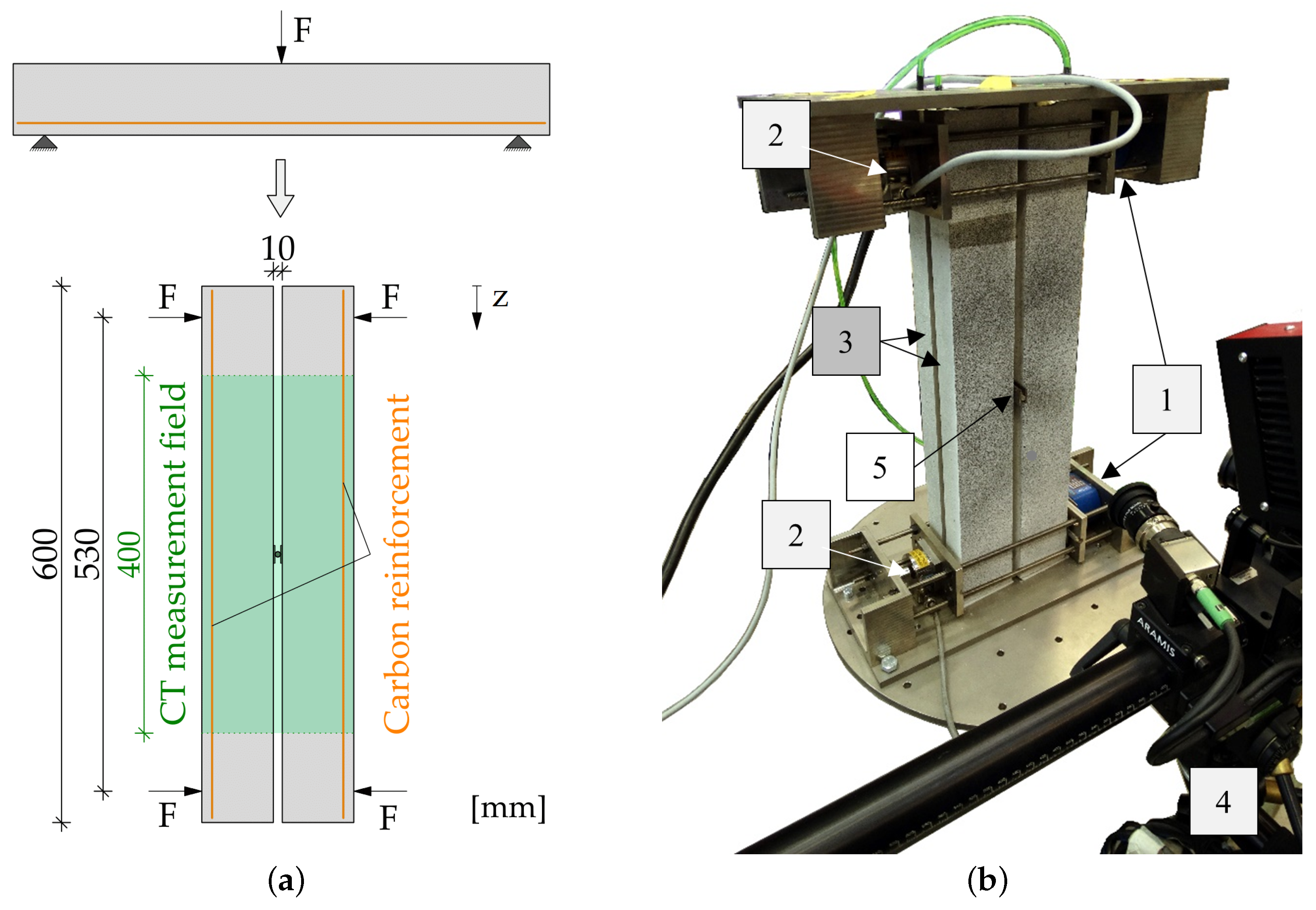
2.1. Test Setup and Experimental Program

The test setup and the experimental program is described in detail in [13]. In the following, a short overview is given:

Figure 1 shows the setup that was utilized for the three-point bending tests, which were performed in an upright position. The tests were carried out on a beam couple (Experiment 1) and a beam quartet (Experiment 2), as illustrated in Figure 2, with a rod in between the beams (gap of 10 mm) that formed the central support. Further information regarding the hydraulic cylinders and load cell configuration can be found in [13].

Due to the size of the utilized CT device, the height of the measurement field was limited to 400 mm, as displayed in Figure 1a. In order to complement the CT data, the half central part of the samples were recorded with a stereo camera system for photogrammetric measurements on the surface.

In the course of the tests, the loads applied by the two cylinders were recorded and summed, to obtain the current load level. CT scans of the samples of each experiment were performed for several load steps (see

Table 1. Load steps for the in situ CT scans. Table adapted with permission from Ref. [13]. 2023, J. Giese.

Load Step	Experiment 1	Experiment 2
0	0 kN	0 kN
1	2 kN	2 kN
2	4 kN	6 kN
3	6 kN	12 kN
4	-	18 kN

). They were previously defined based on preliminary experiments, aiming at capturing different stages of the crack formation. The load level was sustained while scanning. Photogrammetry was used to capture the behavior of the samples during the periods of successive load increase until the next load step was reached.

Before the start of the load application, one CT scan was made of the beams in their initial state (load step 0). For Experiment 1, three further CT scans were executed, for 2, 4, and 6 kN (load steps 1, 2, and 3, respectively). As the load bearing capacity of the samples in Experiment 2 was higher, due to an increased reinforcement ratio, larger increments were chosen for the load steps, resulting in four scans on load levels of 2, 6, 12, and 18 kN (load steps 1, 2, 3, and 4, respectively).

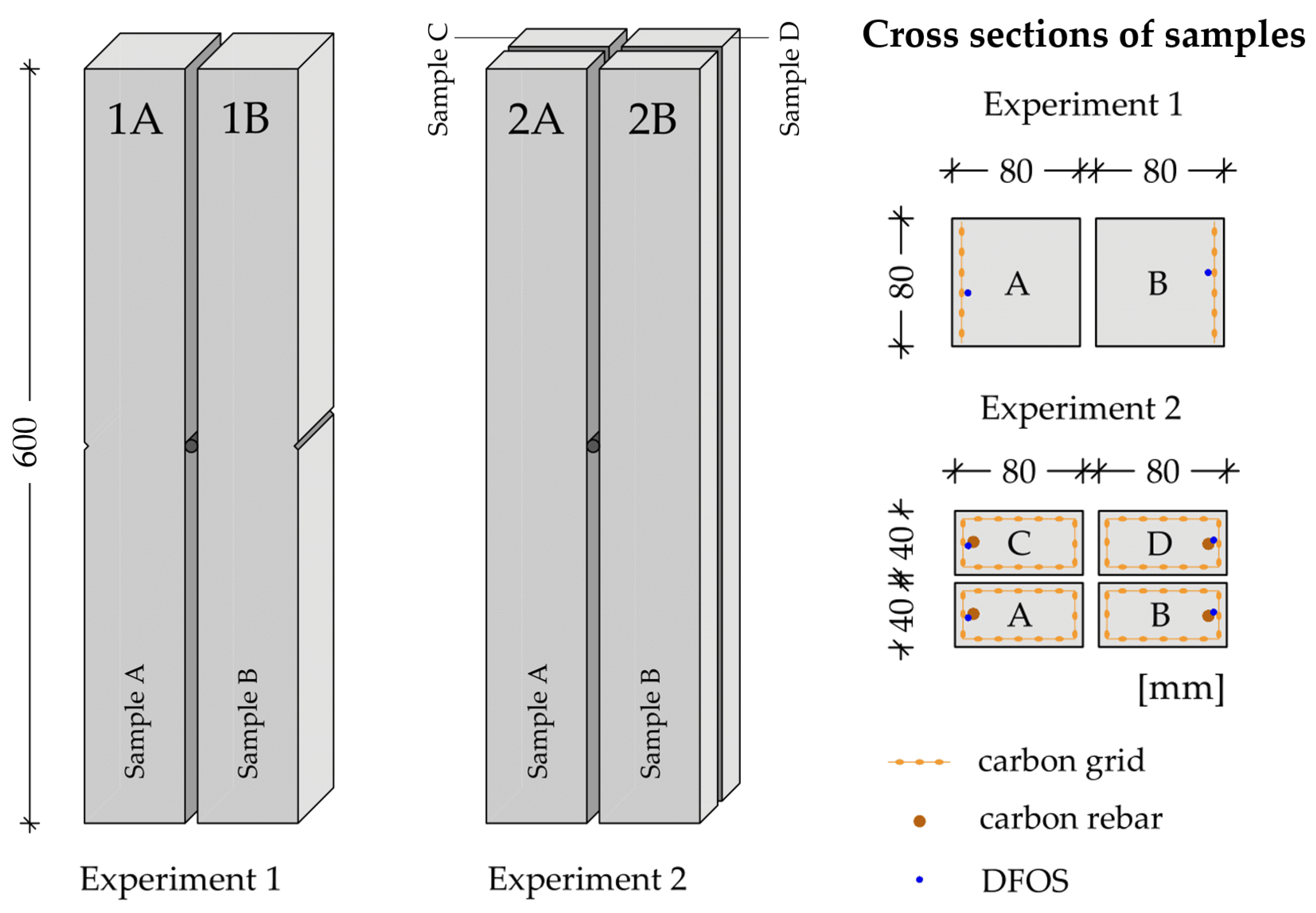
2.2. Specimens

Detailed information about the specimens, including geometry, reinforcement layout, production, and curing, is given in [13]. Here is some brief information:

Two bending tests were carried out on a pair and on a quartet of textile-reinforced concrete beams with a length of 600 mm (Figure 2). From a total of six specimens, two samples had a square cross-section of 80 × 80 mm${}^2$ and an additional notch of 3 mm in the middle of the specimen length for the initialization of the crack (Experiment 1), while four samples had a rectangular cross-section of 80 × 40 mm${}^2$ (Experiment 2).

As shown in Figure 2, two different reinforcement layouts were chosen, to provoke the development of either a few wide cracks (Experiment 1) or many small cracks (Experiment 2). The specimens of Experiment 1 were reinforced with one layer of a carbon textile grid, resulting in a reinforcement ratio of 1.7‰. For the beams of Experiment 2, a carbon rebar was used as longitudinal reinforcement. Additionally, the textile grid was formed into a reinforcement cage and inserted as shear reinforcement. This configuration led to a much higher reinforcement ratio of 26.8‰. The concrete cover was 5 mm.

Moreover, one distributed fiber-optic sensor (DFOS) was continuously attached to the carbon reinforcement in the tension zone of each specimen for internal strain measurements, which are not part of this paper. However, the estimation of crack widths in this study was performed close to the DFOS position, for comparative purposes.

Detailed information regarding this measurement technique as well as the assessment of the results can be found in [13].

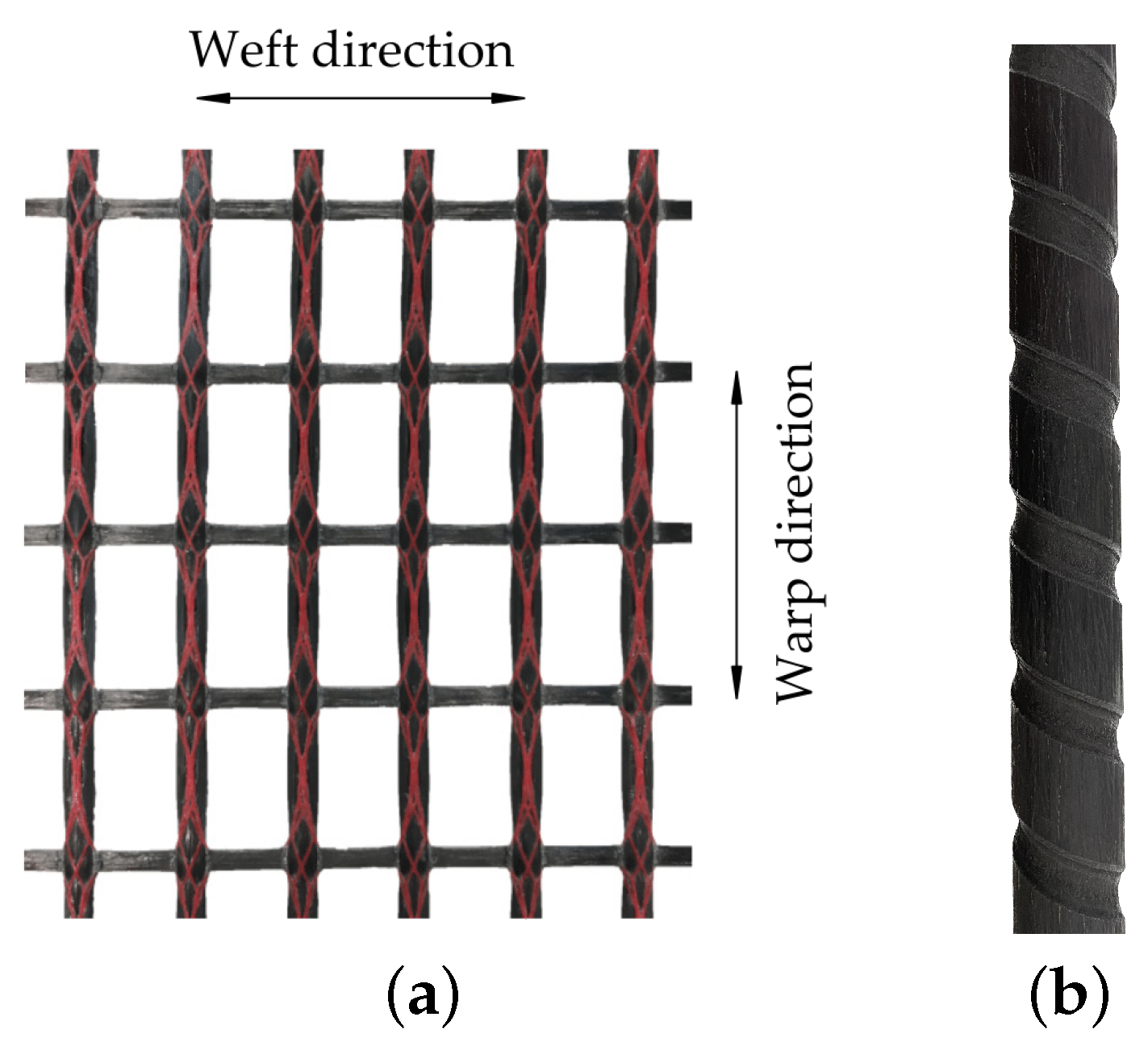
2.3. Materials

The high-strength cementitious matrix utilized for these investigations was self-compacting and contained a maximum aggregate size of 2 mm. Further details about the concrete mixture, which was explicitly developed for use in CRC, are given in [13]. The compressive strength and bending tensile strength were determined on standard prisms (160 × 40 × 40 mm${}^3$) cast together with the beams to 107.4 MPa and 11.4 MPa, respectively. The mean modulus of elasticity of the cementitious matrix has been investigated in previous studies on cylindrical specimens (height–diameter ratio h/d = 300 mm/150 mm) and determined to about 44,000 MPa.

Regarding the planar textile reinforcement, a bidirectional warp-knitted grid made of carbon fiber yarns with a polyacrylate coating was used (Figure 3a). Due to different fiber strand spacings and cross-sectional areas of the yarns (see

Table 2. Carbon reinforcement characteristics. Parts of the table adapted with permission from Ref. [13]. 2023, J. Giese.

		Grid [14]		Rebar [15]
		Warp Direction	Weft Direction
Axial yarn spacing	in mm	12.7	16.0
Cross-sectional area (yarn/rebar)	in mm${}^2$	1.81	0.45	57
Ultimate tensile strength	in MPa	2200		1650
Ultimate strain	in ‰	11.3		11.0
Modulus of elasticity	in MPa	195,000		151,000

), the reinforcement area in the warp direction was significantly higher (141 mm${}^2$/m) than in the weft direction (28 mm${}^2$/m). As for the bar-shaped reinforcement, a rebar with a grooved profiling made of carbon fibers and an epoxy resin impregnation was utilized (Figure 3b). The core diameter, which also corresponded to the design-relevant diameter, was 8.5 mm, resulting in a reinforcement area of 57 mm${}^2$. Further information about the material properties of the carbon reinforcement can be found in Table 2.

2.4. Measurement Methods

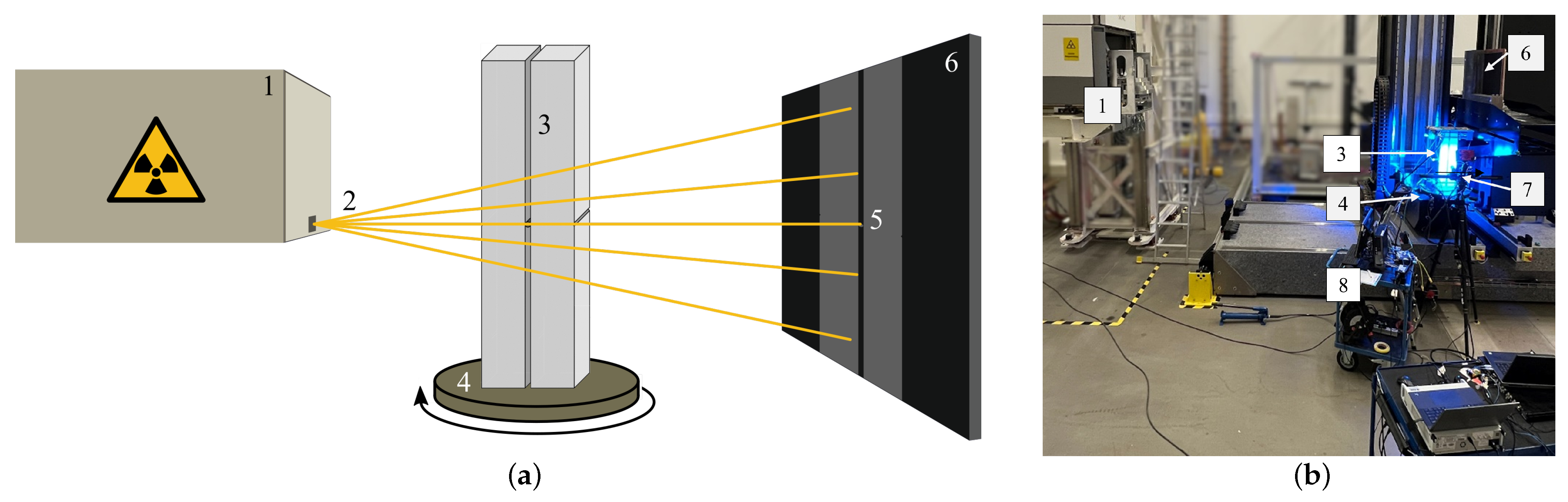
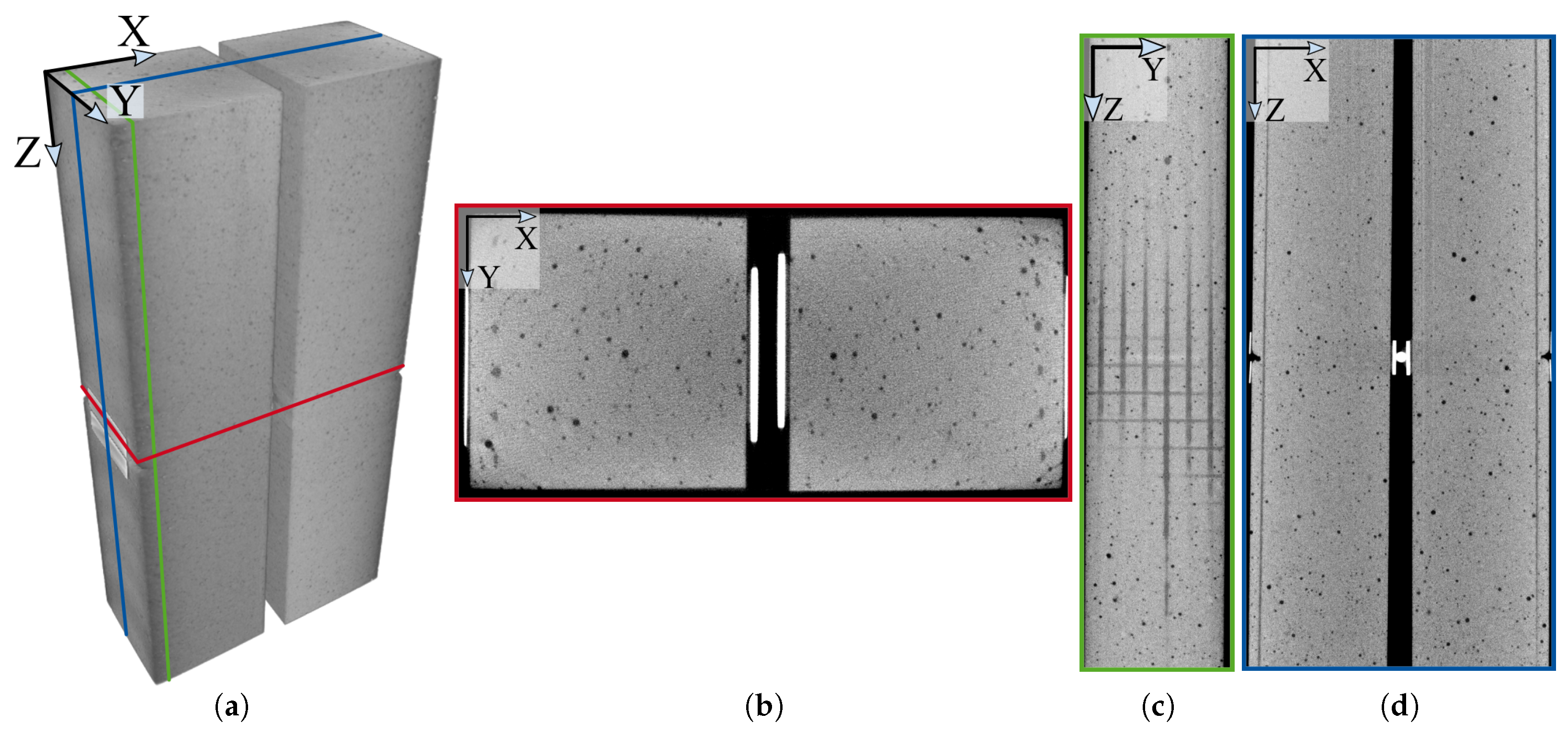
2.4.1. In Situ Computed Tomography

To investigate the inner properties of objects, a CT device can be used (see Figure 4a,b). Such a device consists of an X-ray source (1), a sample (3), and a detector (6). In the process of scanning, a sample undergoes either a complete 360° rotation (standard CT scan) or a partial rotation (≥180° (plus the fan beam opening angle) $<360$°), which is called limited-angle computed tomography [16]. During each rotation step, the sample is exposed to radiation (2) and the resulting projection (5) is captured by the detector. Such a projection image is created by capturing the X-ray attenuation data as the X-ray beams pass through the object being scanned. After a CT scan is completed, a 3D volume is reconstructed from the projections. The resulting 3D reconstruction is typically composed of a series of 2D images stacked together. In this context, a pixel in a 2D image corresponds to a voxel in the 3D volume.

Traditionally, CT takes a static snapshot of an object before it is removed from the CT. For dynamic processes, on the other hand, a scan would be taken before and after performing an experiment outside of the CT device. However, due to the requirements of this experiment, which involved a dynamic process and an immobile experimental setup, a standard CT scan was not appropriate. Instead, the test setup allowed the object and its experimental setup to remain unchanged between two consecutive CT scans. CT that supports such a setup can be referred to as an “in situ CT”.

The tests were conducted at the in situ CT of the Fraunhofer EZRT in Fürth, Germany. As a radiation source, a linear accelerator (linac) with a current of 500 mA and energy of 8.0 MeV was used. The detector was a flat-panel detector of the tomography portal Gulliver from RPTU Kaiserslautern. Each projection image had a resolution of 3072 × 3072 pixels (pixel size: 13 µm and sensitive area of 400 × 400 mm${}^2$). The test rig and the samples (Figure 1) were placed on the rotating platform in between the linac and the detector. The number of projections was limited by rotating the specimens by only 200°. For each scan, 1300 projections were taken, which took approximately 20 min. The main advantage of using such a limited-angle scan is faster imaging, which is crucial to reducing creep effects due to sustained loading. However, when limited-angle data are used, the reconstructed image may contain streak artifacts, blurring or distortion. These artifacts can make it difficult to properly interpret, process, and analyze the images. In addition, the maximum path to be traversed through the objects by a photon is ≈19 cm, which explains the need for the high power. However, the use of high energy comes at a cost, as it tends to introduce significant noise into the reconstructed images. In addition, fine elements of similar density may become indistinguishable from each other, resulting in a loss of detailed information in the CT images [12].

2.4.2. Photogrammetry

In this publication, photogrammetric measurements were also applied, to validate the results of the CT data analysis. A stereo camera system allowed the contactless and precise observation of the surface of one side of the specimens with a high spatial and temporal resolution. In the experiments, the cameras were positioned at a distance of 98 mm with an angle of 25° between them. The operating distance was 30 cm. The system included lenses with a focal distance of 12 mm. For the measurement volume, a CP20 250 × 200 calibration object from the company GOM with a dimension of 25 × 20 cm${}^2$ was selected, in order to determine the relative and inner orientation of the stereo system. The calibration process was performed at constant room temperature and constant light [17]. Blue LED light was used to maintain uniform measurement conditions without heating. After setup and calibration, the test was started and a stereo image sequence was recorded. The area of the observed surface was 17 cm × 30 cm. In the calibration, there was a scale contradiction of 0.001 mm between the two scale distances and a calibration error of 0.045 px (corresponding to 3.4 µm).

2.5. Analysis Methods

2.5.1. Digital Image Correlation

The analysis of the stereo image data was performed using digital image correlation (DIC) [18]. For this purpose, the commercial software GOM ARAMIS (version 2022) was used to compute displacement and strain fields. In addition, the method presented in [19] was applied to measure deformations. Herein, the displacement field was triangulated into a mesh and the triangles were analyzed with regard to changes between the load stages. The model included a split of the triangle and a relative shift ${\overrightarrow{t}}_{rel}$ between the parts. The value of $|{\overrightarrow{t}}_{rel,2D}|$ was used as scalar deformation and the vector ${\overrightarrow{t}}_{rel}$ itself as a 3D deformation vector on the surface. The detection of crack triangles was performed by applying a thresholding to the scalar deformations $|{\overrightarrow{t}}_{rel,2D}|$. The study presented in [19] also proposed an algorithm to automatically derive the crack widths as the projections of the vectors ${\overrightarrow{t}}_{rel}$ onto the crack normals. Liebold et al. [19] also validated their method in [19], so that it could be used as a reference for the volume data analysis. The accuracy of the DIC point measurements in this study was supposed to be a tenth of a pixel, corresponding to 7.5 µm in object space and to 0.06 vx of the CT data.

2.5.2. Digital Volume Correlation

In contrast to image analysis of surface measurements, CT data enable the view inside the specimen. A series of CT datasets, such as those obtained by in situ CT tests [11], can be used for change detection. A popular subvoxel-accurate method for this is the digital volume correlation (DVC) [7], which is an extension from DIC to voxel data. Like DIC, DVC also requires a suitable texture in the CT image data. The deformation measurement and crack detection when using DVC is often performed by computing strains [20]. In this publication, the crack measurement and analysis were done by applying the method of Liebold and Maas [21] with another deformation model that also allowed the automatic determination of crack widths.

The first step was the computation of a subvoxel-precise 3D displacement field by means of the method presented in [22]. The points of the displacement field were triangulated in a tetrahedral mesh and each tetrahedron was analyzed for changes between load steps. The model involved splitting the tetrahedron into two parts, with a relative translation between the parts where two cases were distinguished. This relative shift ${\overrightarrow{t}}_{rel}$ was used as a deformation vector, and the norm of it, $|{\overrightarrow{t}}_{rel}|$, served as a scalar deformation that helped to identify tetrahedra with a crack by applying a thresholding.

In contrast to the method of [21], the crack width detection was done by profile analysis in this publication, due to the high noise in the CT image data. At user-defined profiles, the crack width measurement was performed as follows: First, deformed tetrahedra, where the scalar deformation exceeded a user-defined threshold, were detected along the profiles. Then, the deformed neighbors of these were included, to compute a median vector of the deformation vectors. The norm of the median vector was used as the crack width.

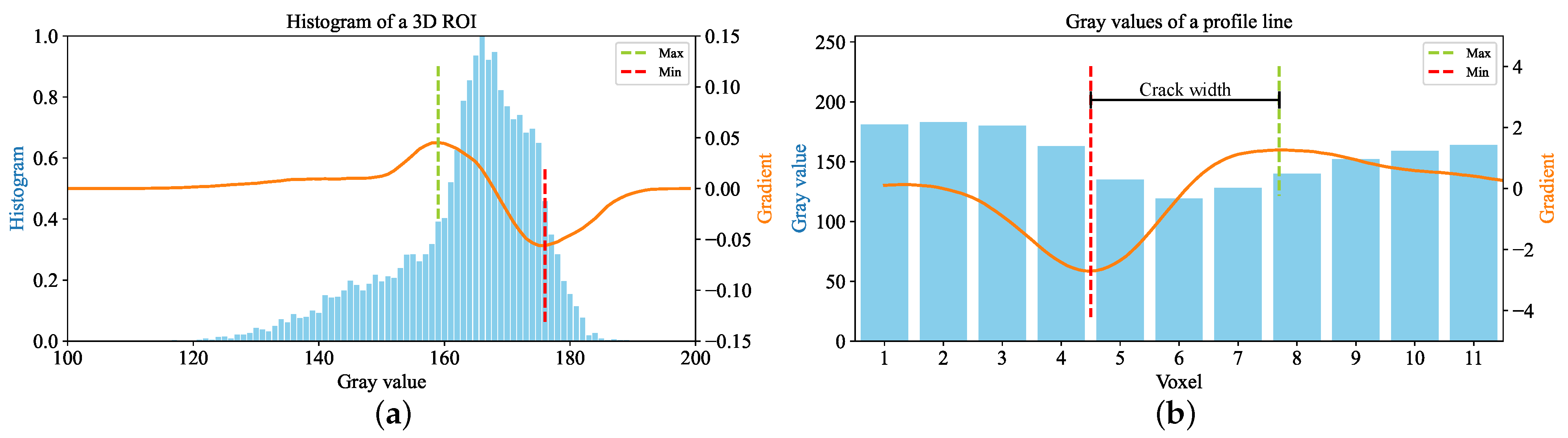
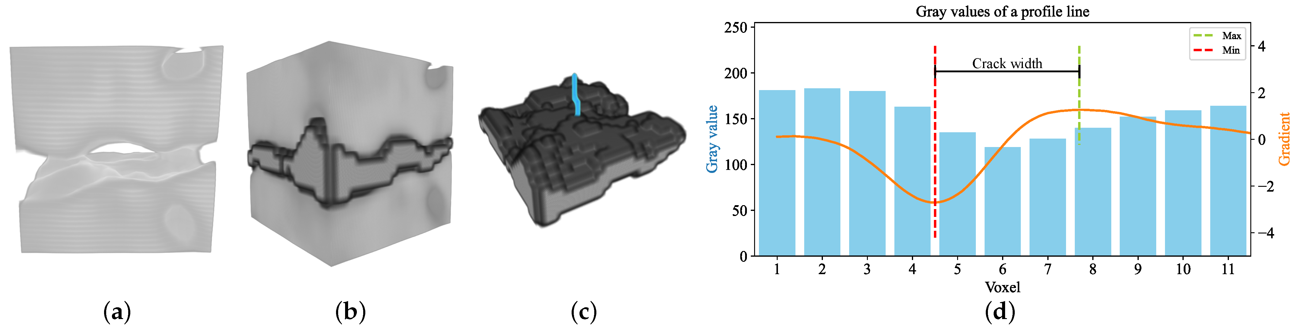
2.5.3. Crack Width Estimation by Grayscale Profile Analysis

Due to the noise caused by the high energy present in the CT reconstructions (compare Section 2.4.1), a substantial amount of structural detail in the image space is lost. Consequently, an evaluation using DVC may fail. Furthermore, DVC necessitates a minimum of two distinct time steps, making it particularly suitable for in situ CT scans that are, however, often not a viable option. Therefore, an alternative approach to concrete crack analysis is to derive crack widths from the grayscale differences of the 3D images. This method involves calculating the distances between crack edges, and it is a technique commonly used in the 2D domain [23,24,25] that can be extended to the third dimension.

In [13], various methods for crack width determination were presented, such as a distributed fiber-optic sensor, which was embedded in concrete along the carbon reinforcement. In order to allow for a comparison of the results determined in [13], only a local determination of the crack width using regions of interest (ROIs) is necessary. Therefore, the aim is to determine the crack width close to the DFOS. More complex segmentation methods, such as those presented and compared in [26], are not necessary. Instead, an adaptive thresholding in combination with morphological operations is sufficient. The basic idea is as follows: By measuring the distance between the flanks of a crack, the width can be obtained. To determine the distance, a line orthogonal to a crack can be used. This line can be estimated by calculating the normal to a plane that lies in between the crack flanks. The coordinates where the normal intersects the flanks can be used to compute the crack width. However, the plane and its normal are unknown, but can be estimated using two assumptions:

First, for extremely small subvolumes, it can be assumed that a crack can be approximated by a nearly flat cube. Consequently, the 3D coordinates representing the crack voxels can be used to fit a plane into the crack region, using singular value decomposition. To segment the crack-related voxels, a histogram analysis is performed on the denoised ROI, using a derivative filter, as shown in Figure 5a. By setting a threshold at the maximum gradient minus a small constant, any value below the threshold can be classified as air (cracks and pores) and any value above can be classified as concrete. A morphological opening [27] removes the noise from the binarized volumes and, by using a 3D connected components analysis and the assumption that a crack consists of the most connected voxels, the crack can be segmented.

Second, the gray values of a crack are smaller than the gray values of the concrete matrix (or in other words, in CT images, a crack is darker than concrete). Therefore, by moving along an orthogonal to the fitted plane, the gray values are high (brighter) at the first crack flank, low (darker) within the crack region, and high (brighter) at the second flank, indicating that a gradient analysis can be used to determine the coordinates where the normal intersects both crack flanks, as illustrated in Figure 5b.

To summarize, the following steps have been concatenated:

• Reduction of noise, using a non-local means filter (only for noisy data);
• Manual selection of ROIs;
• Segmentation of the crack;
• Plane fit to the crack voxels;
• Calculation of the profile along the normal;
• Measurement of the distance between the minimum and maximum gradient.

However, even at such a small scale, the surface of a crack is expected to be quite complex and a single profile line may not be sufficient. Therefore, several normals are added in a circle on the plane around the center normal. For example, using a radius of 5 voxels and an angular step size of 45°, eight additional normals can be employed to approximate the crack width in this particular region.

A major disadvantage of this approach is that a crack must be discernible in the grayscale profile, which is not true for cracks that are smaller than a voxel, given the noise in this study.

2.6. Quality Control

As CT data provide valuable information about the internal structure of the material in a non-destructive manner, they can be used for quality control purposes, primarily involving dimensional metrology, flaw detection, and porosity assessment [28]. Within the scope of this study, the thickness of the concrete cover along the reinforcement elements and the air void distribution inside the beams were examined. In 3D data from CT scans, it is possible to segment these phenomena that cannot be obtained by other measurement methods [29]. However, as explained in Section 2.4.1, the 3D reconstructions have challenging properties, such as high noise and varying grayscale ranges.

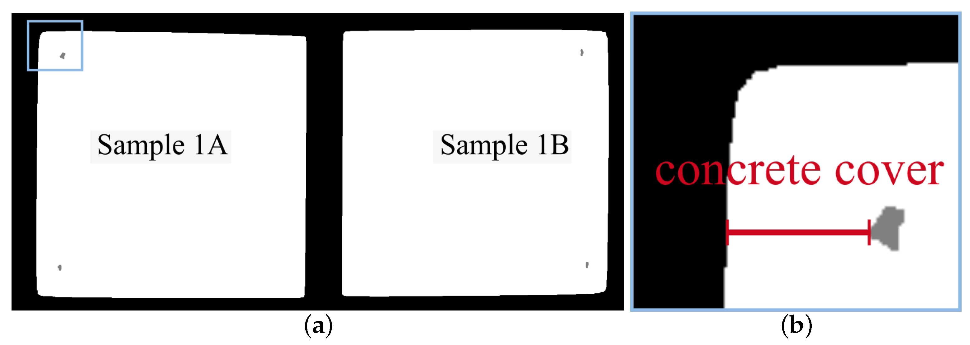
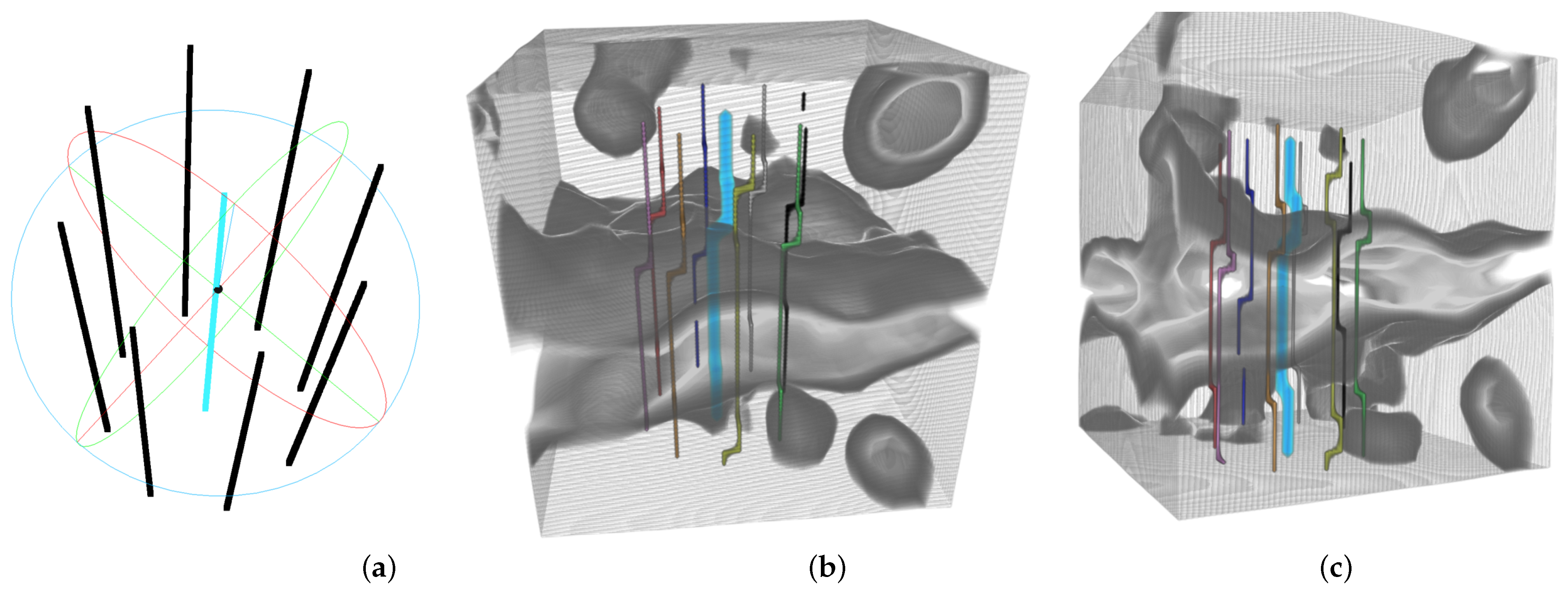
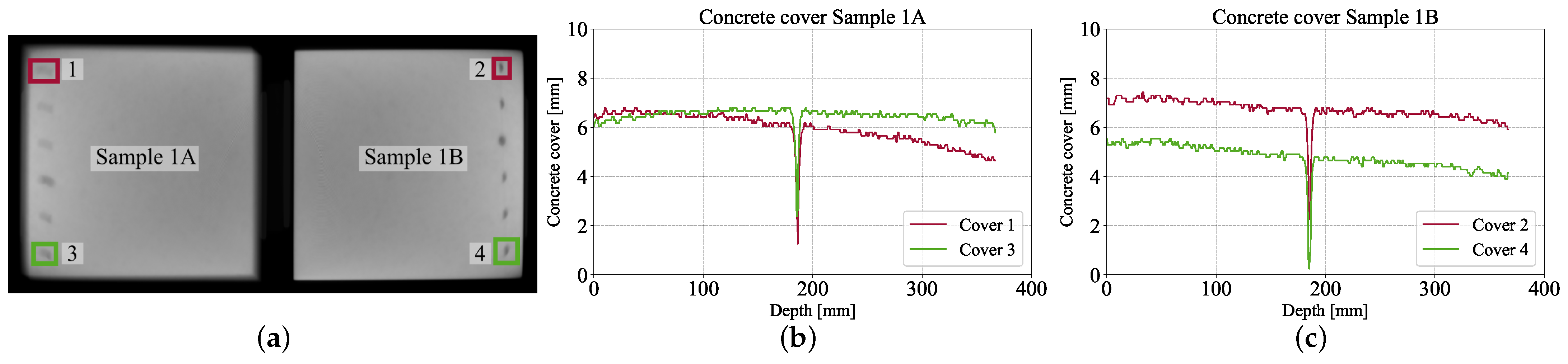
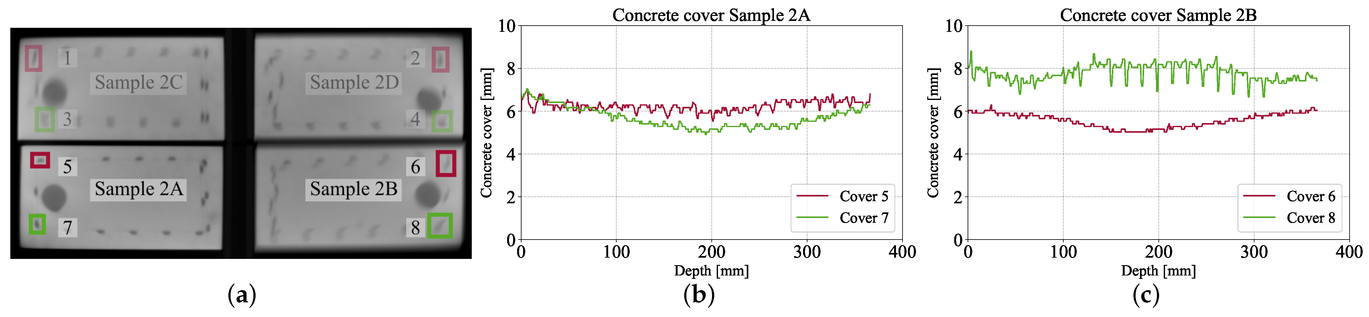
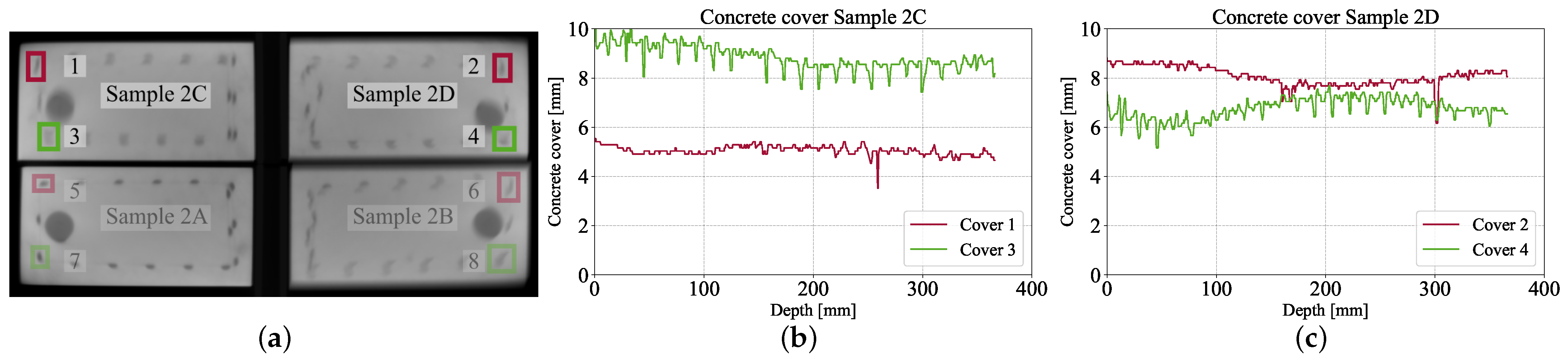
2.6.1. Analysis of Concrete Cover

According to Eurocode 2 [30], the concrete cover is defined as the distance between the surface of a rebar and the nearest concrete surface. This specification may also be used for concrete constructions with non-metallic reinforcement (grid or rebar). Unlike steel reinforcement, the purpose of the concrete cover does not include corrosion protection, as the non-metallic reinforcement is not susceptible to corrosion. However, sufficient concrete cover is required, in order to safely transmit bond forces between the reinforcement and surrounding concrete, prevent concrete spalling, and ensure fire protection. As the beams were manufactured under laboratory conditions and only for experimental purposes, the minimum value of 5 mm according to [31] was chosen for the concrete cover. The position of the reinforcement within the hardened concrete matrix is traditionally determined by inspection and measuring of saw cut planes, e.g., [32]. However, CT allows the non-destructive visualization and localization of reinforcement materials and can therefore be used to evaluate if the intended concrete cover is maintained along the z-axis of the beams.

As the carbon can be easily distinguished from the concrete matrix in CT images, it is possible to extract it automatically. To estimate the distance of the outer edge to a single roving, it must first be segmented. This is done by histogram analysis of a ROI around the carbon. The ROI is chosen manually, in such a way that the subvolume, which extends over the entire depth (z-direction) of the volume, contains only a single roving and a fragment of concrete. As the carbon is represented by lower gray values than the concrete (carbon reinforcement is visually darker on the images), the histogram should contain two peaks: one representing the average gray value of the carbon and one representing the average gray value of the concrete.

To segment the carbon reinforcement, the minimum value of the valley between these peaks is used as a threshold. Values below are then classified as roving, values above as concrete. Air is also removed by applying another thresholding. Once the carbon has been segmented, the whole samples also had to be binarized, which was done by a simple thresholding and the floodfill algorithm. As shown in Figure 6b, the distance from the leftmost voxel of the carbon to the concrete surface was measured.

2.6.2. Porosity

Porosity is a measure of the voids or gaps within a material, and it is often used to evaluate the quality of concrete. It indicates how much of the volume of the concrete consists of open pores, which can affect properties such as strength, durability, and permeability. There are several methods for estimating porosity in concrete, such as the water absorption test [33], mercury intrusion porosimetry [34], or image [34] and volume analysis [35]. Due to the three-dimensional nature of the CT data, volume-based porosity analysis was performed in this study. However, in order to measure the porosity of the concrete, the pores had to first be segmented.

Pore Segmentation: The segmentation of pores and air voids in the CT data of concrete probes is a well-known and often-described operation, as the air should be almost black (gray value near or equal to 0) because of its high transmittance. However, due to varying gray values and high noise, the pores in the sample were not easily extractable. Because many pores have gray values similar to carbon, and because of their small size and noise, it is difficult to automate the process reliably, even for a single image. Therefore, more advanced, automated thresholding methods were tested, using Dragonfly (version 2021.1) from Object Research Systems (ORS): Adaptive Threshold, the ISODATA method, and Otsu.

Although the ISODATA method achieved the best results of those three, the results were still not sufficient, as many pores were missing. Therefore, a 3D U-Net [36] was trained, using the AiSeg project (https://gitlab.com/fra-wa/aiseg, accessed on 10 October 2023) and a public pore segmentation dataset (https://doi.org/10.34740/KAGGLE/DS/2921245, accessed on 10 October 2023). This CNN has been shown to perform best on this segmentation task [37]. However, the dataset contains several good-quality CT scans where the pores are trivial to detect. Therefore, data augmentation techniques were needed, to tune the variance of the dataset, so that the CNN could generalize well enough to segment the pores that occurred in this study. In [38], 3D data augmentation pipelines were introduced to the AiSeg project, and these were consequently adapted to the needs of this investigation.

To evaluate a CNN in segmentation tasks, it is common to use the F1 score (also known as the DICE coefficient or overlap index). This measure provides a balanced way to account for both false positives and false negatives, making it a useful measure in scenarios where class imbalance or misclassification costs are significant [39]. However, as the training dataset consists of error-free CT scans, the result also had to be evaluated visually on the CT data in this study.

Pores Distribution: To quantify the presence of pores in CT data, one method is to calculate the ratio of voxels classified as pores to all voxels per cm${}^3$. The resulting percentage provides comparable values that can be analyzed against the casting process: as the concrete was poured into a vertical formwork in the z-direction (Section 2.1, Figure 1), the distribution could be analyzed in relation to the pouring process.

3. Results

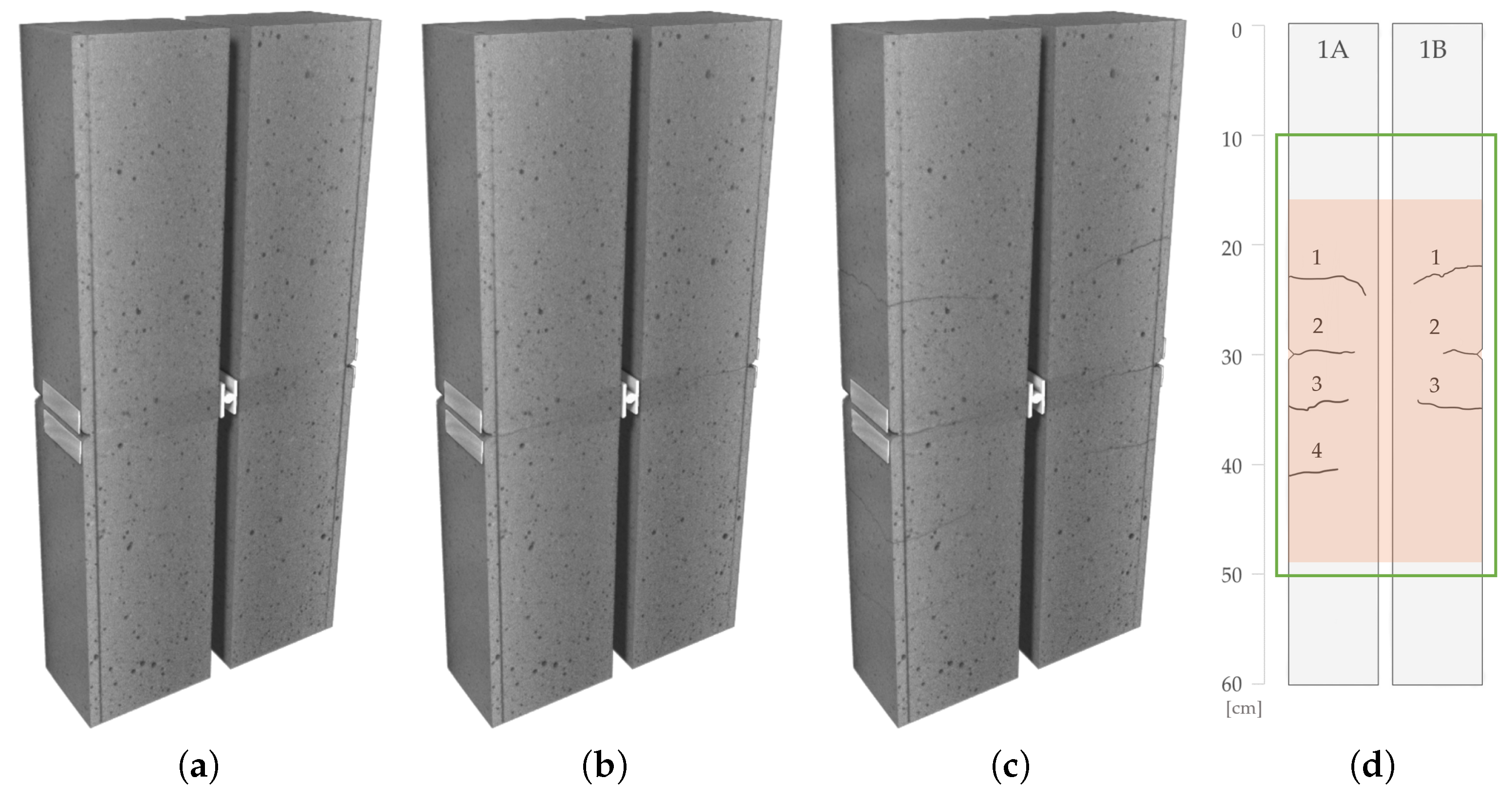
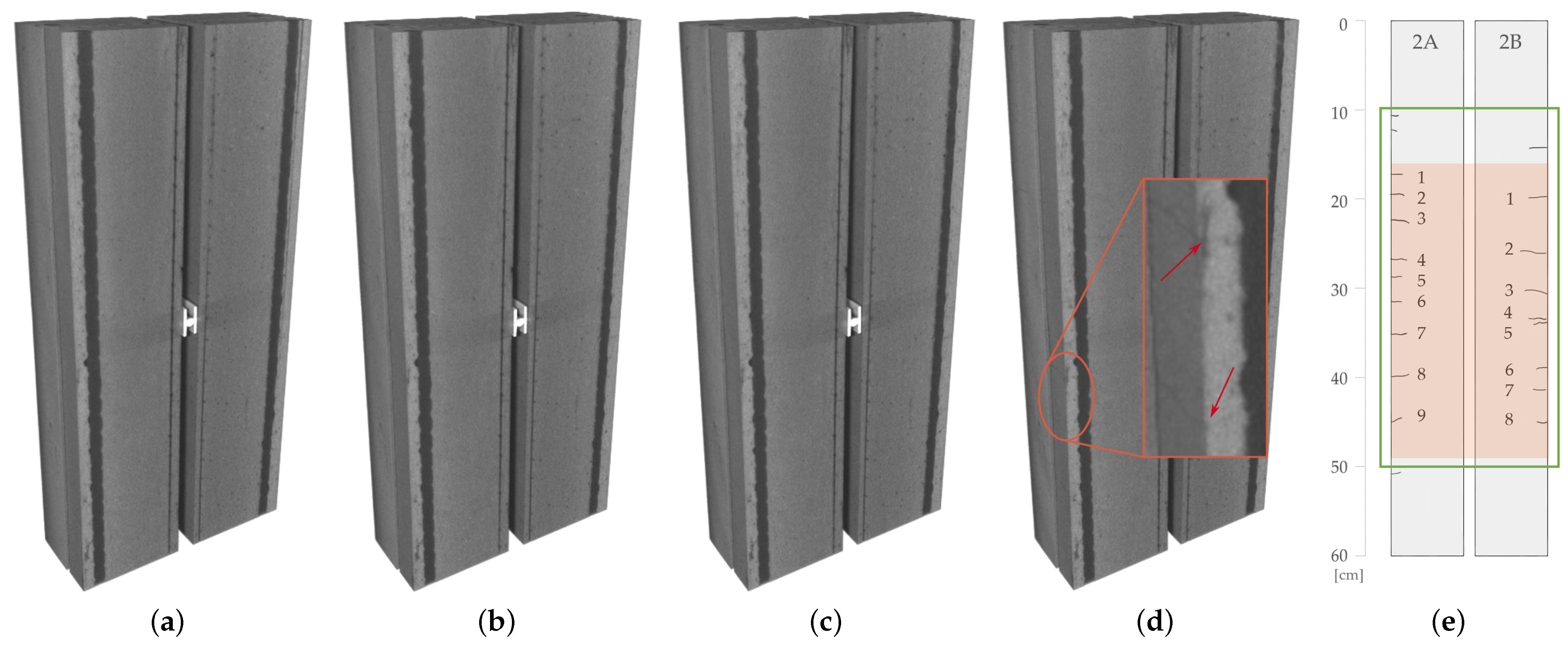
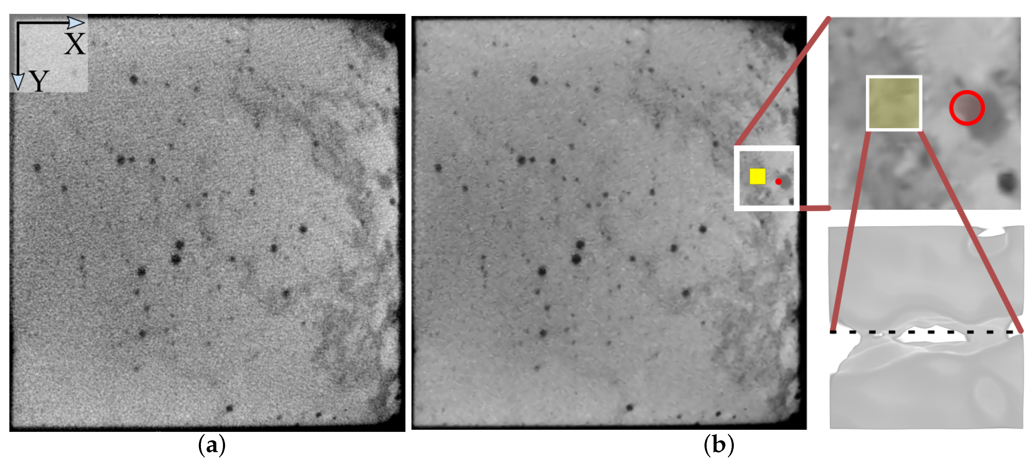
3.1. In Situ CT Scans

Figure 7 shows a 3D reconstruction of Experiment 1 (under zero-load) with the positions of the cross-sectional images marked. As mentioned in Section 2.4.1, several factors contributed to the noisy nature of the images. Despite the lack of distinguishable constituents in the concrete, due to the high power and scan settings, the carbon remains visible.

Figure 8 and Figure 9 show the two experiments at different load stages. In Figure 8b,c the evolution of multiple cracks is visible. Figure 8d and Figure 9d depict sketches of the crack pattern with numbering. In addition, the area of the photogrammetric measurement is colored in orange and the green frame stands for the measuring field of the CT.

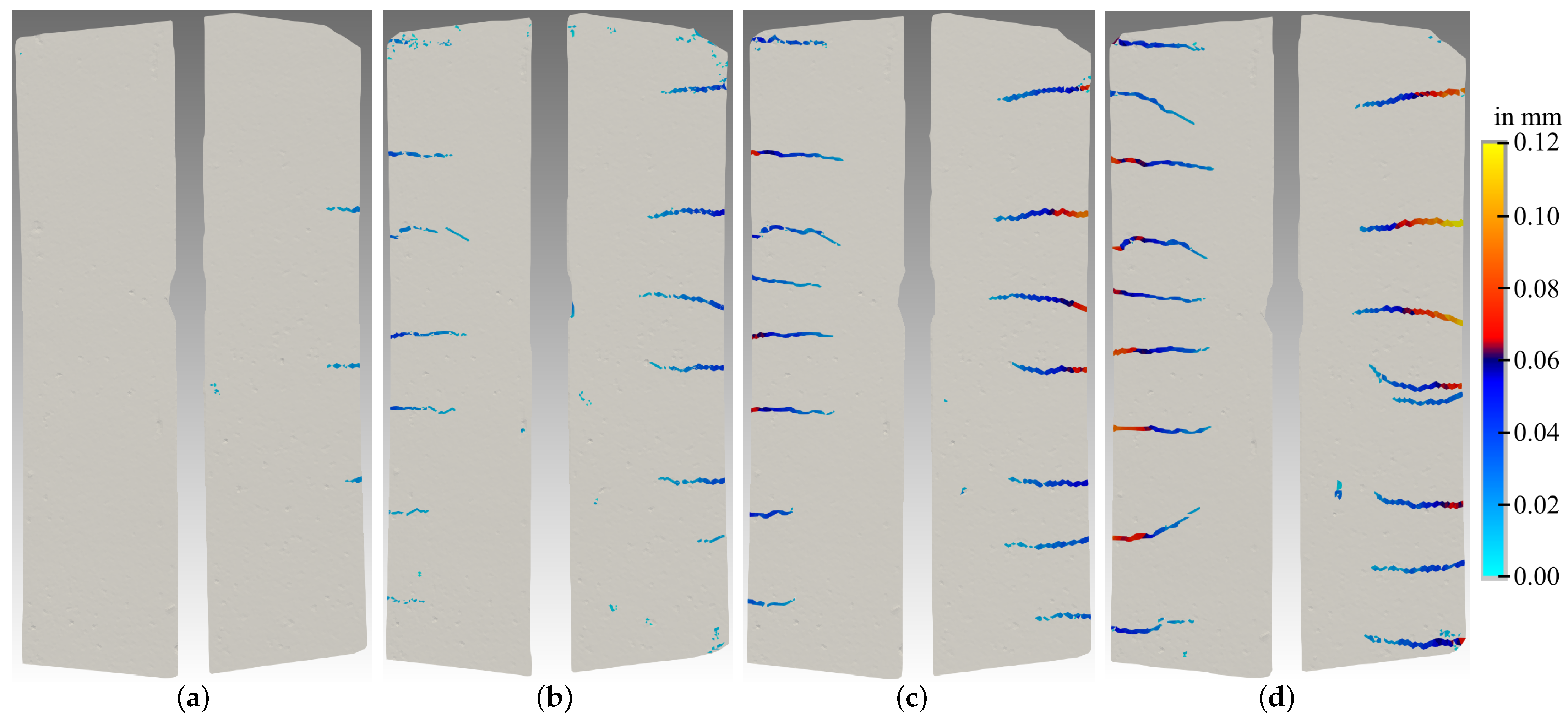
3.2. Digital Image Correlation

As mentioned in Section 2.5.1, DIC was applied to the stereo image sequences that observed one side of the surfaces of each sample. The results of Experiment 1 are shown in Figure 10 and Figure 11. Figure 10 depicts the color-coded triangular mesh representing the scalar deformation field as well as the deformation vectors, as used by Liebold et al. [19] for the three load steps. At a load of 4 kN, one crack was detected on each sample at the notches. At the next load step of 6 kN, three more cracks on the left side and two more cracks on the right side appeared.

Crack triangles were determined by applying a thresholding (threshold $\delta =0.02$ mm) to the scalar deformation quantity. Then, crack widths were computed and are shown as a color-coded visualization for the crack triangles in Figure 11. At the notches, the crack widths were ca. 0.2 mm on both sides at the load step of 4 kN and ca. 0.3 mm for the load step at 6 kN.

Table 3 shows the crack widths [mm] of the DIC analysis for Experiment 1 at a distance of 5 mm to the left and right outer edge of the specimens.

Table 3. Crack widths in mm of the DIC analysis for Experiment 1 at a distance of 5 mm to the outer edge for the load steps of 4 kN and 6 kN. The cracks are labeled as shown in Figure 8d.

	Load Step at 4 kN		Load Step at 6 kN
Crack Label	1A	1B	1A	1B
1			0.224	0.270
2	0.168	0.203	0.272	0.300
3			0.198	0.227
4			0.132

Table 3. Crack widths in mm of the DIC analysis for Experiment 1 at a distance of 5 mm to the outer edge for the load steps of 4 kN and 6 kN. The cracks are labeled as shown in Figure 8d.

	Load Step at 4 kN		Load Step at 6 kN
Crack Label	1A	1B	1A	1B
1			0.224	0.270
2	0.168	0.203	0.272	0.300
3			0.198	0.227
4			0.132

The DIC results of Experiment 2 are shown in Figure 12 (deformation scalar and vector field) and Figure 13 (detected cracks with widths). Due to the higher reinforcement ratio of the samples, more but significantly smaller cracks (maximum crack width of 0.126 mm) appeared, consequently resulting in reduced spacing between the cracks, compared to Experiment 1.

Table 4. Crack widths in mm of the DIC analysis for Experiment 2 at a distance of 5 mm to the outer edges for the load steps of 2 kN, 6 kN, 12 kN, and 18 kN. The cracks are labeled as shown in Figure 9e.

Load	2 kN		6 kN		12 kN		18 kN
Label	2A	2B	2A	2B	2A	2B	2A	2B
1			0.025	0.035	0.052	0.059	0.057	0.081
2		0.018		0.048		0.092	0.030	0.126
3			0.027	0.034	0.053	0.066	0.062	0.100
4		0.016	0.019	0.039	0.025	0.069	0.048	0.072
5					0.028		0.059	0.030
6		0.013	0.039	0.035	0.067	0.053	0.081	0.066
7			0.030	0.017	0.053	0.029	0.083	0.032
8			0.017		0.033	0.022	0.064	0.048
9			0.012		0.026		0.053

contains the crack width values for the labeled cracks at a distance of 5 mm to the outer edges of the measurement surface according to the different load steps.

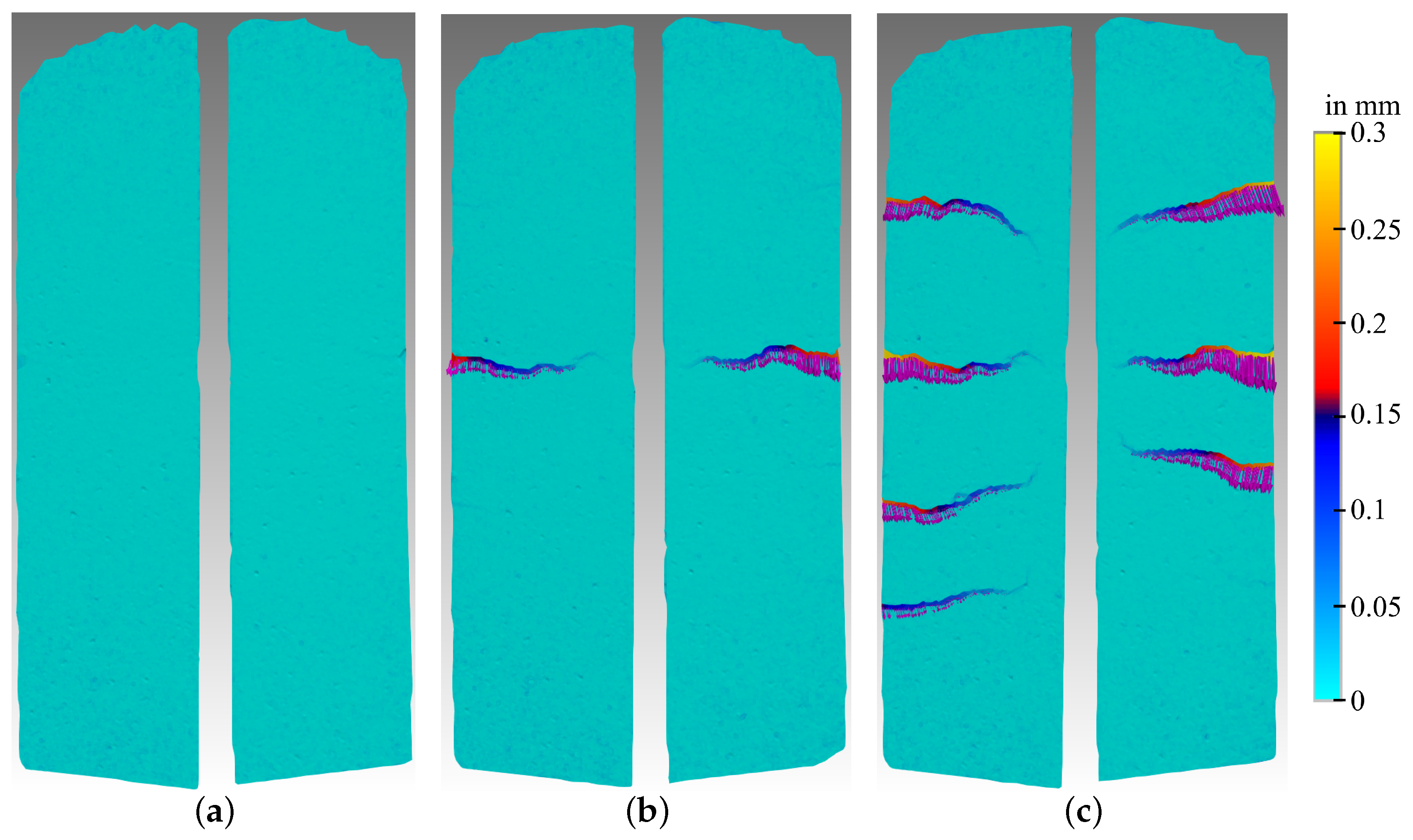
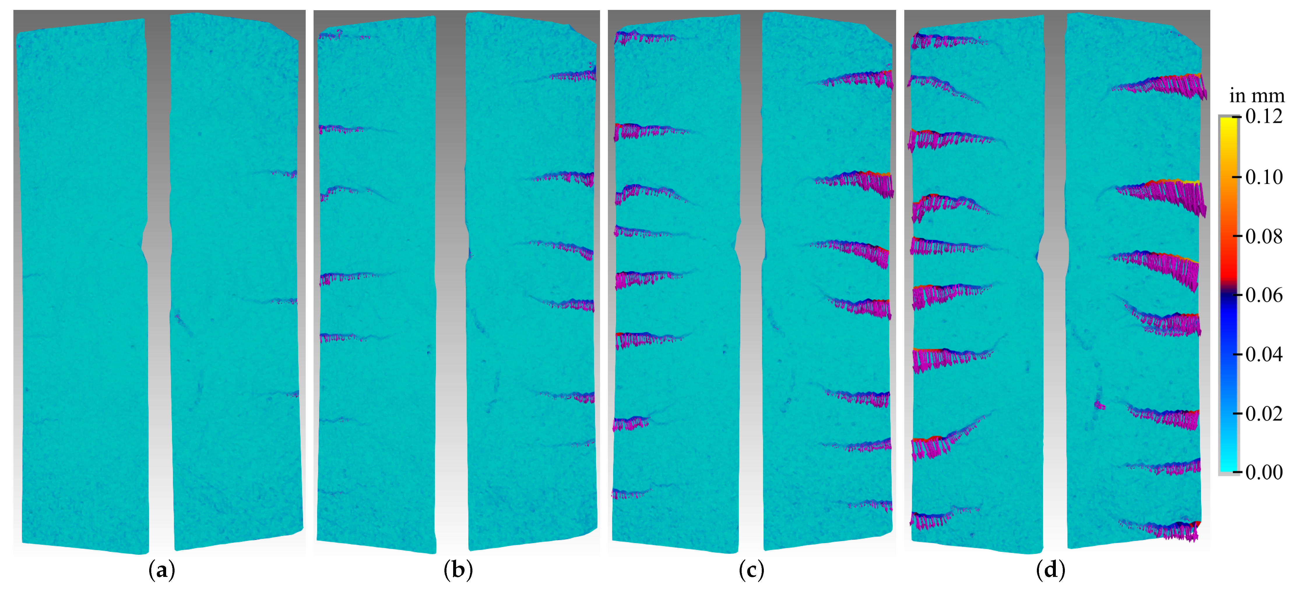
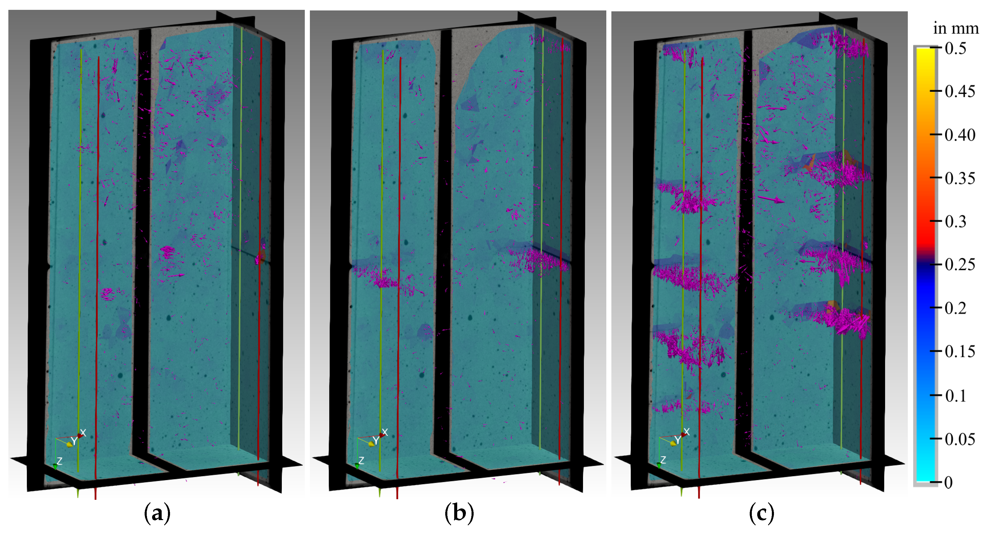
3.3. Digital Volume Correlation

As indicated in Section 2.5.2, DVC was applied to the in situ CT datasets. Due to the high noise and the lack of texture, the dataset was resampled by half. This also reduced the calculation time. For the computation of the displacement fields, subvolumes of 25 × 25 × 25 vx (vx: voxels) were used for a grid of 20 vx spacing in the downscaled data. This was followed by the triangulation to a tetrahedral mesh. The threshold for the detection of deformed edges was set to 0.4 vx. This value was used to distinguish cases for the tetrahedron splitting in the algorithm of [21]. Figure 14 shows a visualization for Experiment 1. It depicts three cross-sections through the voxel data and, additionally, the cross-sections through the transparent color-coded tetrahedra that represent the $|{\overrightarrow{t}}_{rel}|$ values (scalar deformation quantity used by [21]). Furthermore, the deformation vectors (the vectors used by [21]) are shown. At load step 2 (4 kN), one crack was visible at the notch for each specimen, identifiable by the clustered magenta deformations vectors. At load step 3 (6 kN), several cracks formed in the tension zone of the beams. The clusters of deformation vectors at the top of the samples in Figure 14c were ignored because they were artefacts due to errors in the CT reconstruction at the boundary area.

In Figure 14, the green lines represent the position of the DFOS attached to the carbon reinforcement (see Section 2.2). At these profiles, the crack width measurement was performed as described in Section 2.5.2. Along the profiles, deformed tetrahedra, where the scalar deformation exceeded 1.2 vx, were detected and the norm of the median vector of candidates and its deformed neighbors was computed. Table 5 shows the results of the crack width determination (the norm of the median vectors) for the different load steps for the green profiles.

Table 5. Crack widths $w_{DVC}$ in mm of the DVC analysis for Experiment 1 along the green profiles for the load steps at 4 kN and 6 kN. The cracks are labeled as shown in Figure 8d.

	Load Step at 4 kN		Load Step at 6 kN
Crack Label	1A	1B	1A	1B
1			0.193	0.254
2	0.247	0.212	0.268	0.318
3			0.227	0.216
4			0.174

Table 5. Crack widths $w_{DVC}$ in mm of the DVC analysis for Experiment 1 along the green profiles for the load steps at 4 kN and 6 kN. The cracks are labeled as shown in Figure 8d.

	Load Step at 4 kN		Load Step at 6 kN
Crack Label	1A	1B	1A	1B
1			0.193	0.254
2	0.247	0.212	0.268	0.318
3			0.227	0.216
4			0.174

A second profile analysis (red profiles in Figure 14) was done near the surface of the photogrammetric measurements, in order to compare the values to the crack widths from the DIC method, see Table 6.

Table 6. Crack widths $w_{DVC}$ in mm of the DVC analysis for Experiment 1 along the red profiles for the load steps at 4 kN and 6 kN. The cracks are labeled as shown in Figure 8d.

	Load Step at 4 kN		Load Step at 6 kN
Crack Label	1A	1B	1A	1B
1			0.290	0.293
2	0.172	0.219	0.252	0.301
3			0.202	0.289
4			0.245

Table 6. Crack widths $w_{DVC}$ in mm of the DVC analysis for Experiment 1 along the red profiles for the load steps at 4 kN and 6 kN. The cracks are labeled as shown in Figure 8d.

	Load Step at 4 kN		Load Step at 6 kN
Crack Label	1A	1B	1A	1B
1			0.290	0.293
2	0.172	0.219	0.252	0.301
3			0.202	0.289
4			0.245

As mentioned above, the DIC measurements were used as reference, to validate the CT data analysis.

Table 7. Differences of crack widths $\Delta =w_{DVC}-w_{DIC}$ in mm of the profile analysis of the DVC and the DIC of Experiment 1.

	Load Step 2 (4 kN)		Load Step 3 (6 kN)
Crack Label	1A   $\Delta$  in mm	1B   $\Delta$  in mm	1A   $\Delta$  in mm	1B   $\Delta$  in mm
1			0.066	0.023
2	0.004	0.016	−0.020	0.071
3			0.004	0.062
4			0.113

shows the differences $\Delta$ between the DVC profile analysis and the DIC measurements for Experiment 1 (difference between Table 3 and Table 6). The median deviation was 0.023 mm, which corresponded to ca. 0.2 vx. The root mean square error (RMSE), as a further measure of accuracy, was 0.055 mm (0.44 vx).

Due to lack of texture, DVC could not be performed successfully for Experiment 2. Nevertheless, the next section presents a method that can measure crack widths in structureless CT scans if cracks are large enough.

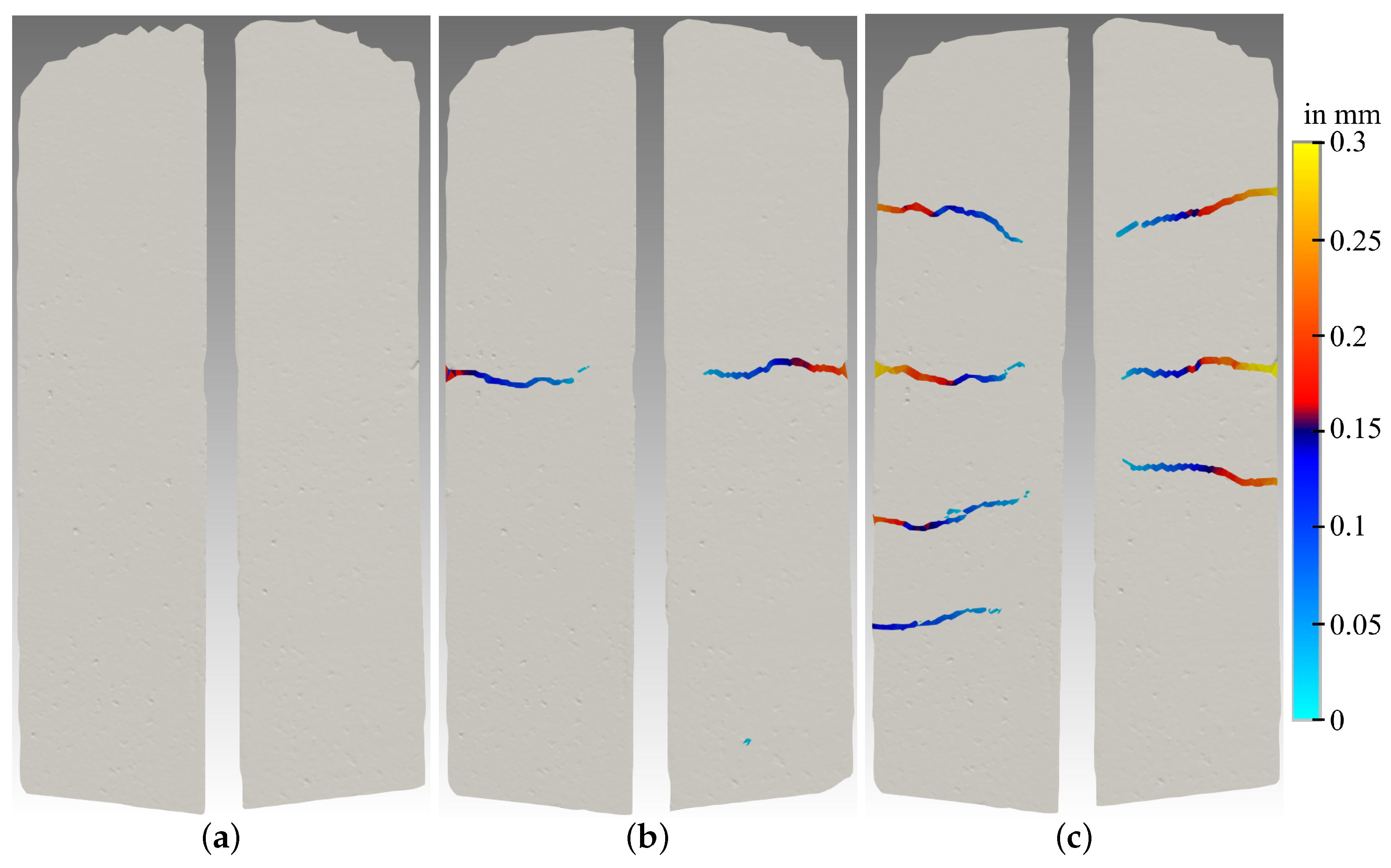
3.4. Grayscale Profile Analysis

The grayscale profile calculation followed the procedure described in Section 2.5.3. First, a 3D non-local means (NLM) filter was applied, to significantly reduce noise (Figure 15a vs. b). The standard deviation of the gray values corresponding to the concrete matrix before applying the NLM filter was 22.4, and after noise reduction it was 13.6, which was still very high. Then, the ROIs were selected, with a size of 25 × 25 × 25 (≈31 mm${}^3$) voxels each, on which the further steps were calculated (Figure 15b). All crack ROIs were chosen with their centers within a 5.5 mm distance to the border of the carbon reinforcement and the DFOS, to enable a second comparison of crack widths besides DVC (e.g., marked with a red dot in Figure 15b; for further details, see [13]).

As shown in Figure 8d, a total of seven cracks evolved until load step 3 (6 kN). An example of a crack within its 3D ROI is shown in Figure 16a. The grayscale region representing the crack and pores was extracted from the histogram of the 3D ROI, using a derivative filter with a filter radius of 10 (21 data points), as explained in Section 2.5.3, to smooth the noise. Voxels with a gray value below the maximum gradient minus a small constant of 5 were classified as pores and cracks. By applying the opening operation (mathematical morphology) with a kernel size of 3 × 3 × 3, followed by the connected components analysis with a 26-connection, pores and noise could be removed from the classification, resulting in Figure 16b. Next, the voxels representing the crack were used to compute the best-fitting plane (via singular value decomposition) and to determine the normal (rendered into the voxel space in Figure 16c).

It was known from visual inspection that the crack widths ranged from 1 to 6 voxels. Therefore, the profile length was set to 11 voxels, in combination with a subvoxel accurate step size of 0.1. Starting from the origin, the profile extended to 5 voxels in the negative direction and 5 voxels in the positive direction. For the gradient calculation along the subvoxel accurate profile, the 1D derivative filter with a filter size of 21 (2.1 voxels) was used, to calculate the gradient of the profile, as depicted in Figure 16d.

As shown in Figure 16a and Figure 17b, it can be observed that the crack and its surface exhibited considerable complexity, and that the plane fit provided only a rough approximation. To account for local anomalies, such as pores on the crack flanks, that could affect the crack width, more profiles were added, to estimate the mean crack width in this region. Starting from the central normal, a radius of 5 voxels and an angular step size of 45 degrees were selected, to define the origins of the additional profiles (Figure 17a). For visualization purposes, only the eight profiles were rendered in the voxel space, as shown in Figure 17b,c. Due to the rendering, they could not be represented as lines. In reality, five different radii with $r=\{1,2,3,4,5\}$ were used, resulting in $8\times 5=40$ normals per ROI.

The process was performed automatically for all the cracks, resulting in

Table 8. Crack widths of samples of Experiment 1 for load step 2 and 3 with standard deviations $\sigma$.

	Load Step 2 (4 kN)		Load Step 3 (6 kN)
Crack Label	1A in mm ($\mathit{\sigma }$)	1B in mm ($\mathit{\sigma }$)	1A in mm ($\mathit{\sigma }$)	1B in mm ($\mathit{\sigma }$)
1			0.67 (0.17)	0.52 (0.15)
2	0.49 (0.13)	0.49 (0.14)	0.55 (0.20)	0.48 (0.13)
3			0.55 (0.17)	0.59 (0.15)
4			0.62 (0.21)

showing the crack widths and their corresponding standard deviations. Note that the standard deviations were relatively large, compared to the absolute crack widths. The average standard deviation was 1.24 voxels or 0.16 mm for crack widths from 3.8 to 5.4 voxels (from 0.48 to 0.67 mm). This result is explained by the undulating nature of the crack surface (Figure 17c) and the challenging characteristics of the noisy data. Consequently, estimating the crack widths with subvoxel accuracy using this approach was not practical under these circumstances. Nevertheless, the crack widths appeared visually reasonable on a local scale.

However, there is a noticeable contrast when comparing the results to those obtained using DVC, as presented in

Table 9. Overestimation ($\Delta$) of crack widths of the profile analysis vs. DVC.

	Load Step 2 (4 kN)		Load Step 3 (6 kN)
Crack Label	1A $\Delta$ in mm	1B   $\Delta$  in mm	1A $\Delta$ in mm	1B $\Delta$ in mm
1			0.477	0.266
2	0.236	0.278	0.282	0.162
3			0.323	0.374
4			0.446

. On average, this technique tended to overestimate the crack widths by a median of 0.282 mm. The RMSE was 0.33 mm. As the DIC and DFOS in [13] achieved similar results to the DVC, and this was a rather large discrepancy, it was verified using multiple, manual profile analyses, using the software ParaView (version 5.11), where similar results were observed with both the NLM-filtered and the original CT data. This discrepancy can be attributed to the non-binary nature of the cracks. A crack possess a porous and undulating character rather than a discrete form. Consequently, within the confines of the crack boundaries, there may be regions of the concrete that are less compact, or the crack may pass through a pore, resulting in gradient variations that do not conform to the expected discrete pattern. For example, in Figure 16d, the gradient values between voxel 6.75 and 8.5 are quite similar, with the maximum value possibly not representing the optimal crack flank. Thus, the visual appearance of a crack in a CT image may exaggerate its size, compared to the actual displacement field. For larger cracks, however, the air between the crack flanks should become more apparent and, as shown in several studies in 2D [24,25], the crack width can be estimated with greater confidence.

While this method theoretically provides a valid alternative for estimating crack widths in CT reconstructions lacking temporal information, DVC should be prioritized for multi-temporal datasets, especially when dealing with cracks represented by a small number of voxels and when the structural quality of the reconstruction is sufficiently high.

Improvements to the profile analysis approach could include the use of a more appropriate radiation source, to minimize noise, and the implementation of a neural network for automated coarse crack segmentation. However, this requires the generation of training data, which is time consuming. Unfortunately for Experiment 2 the analysis was not feasible, because the cracks were smaller than 1 voxel (see Table 4) and the standard deviation of the method was larger than the voxel size (≈0.125 mm). In addition, due to the noise and voxel size, the detection of a crack by grayscale profile analysis was difficult, if not impossible, for this particular CT reconstruction.

3.5. Quality Control

3.5.1. Concrete Cover

The concrete cover was determined by calculating the distance between the reinforcement and the sample surface along the z-axis according to [30]. As shown in

Table 10. Mean concrete cover of all samples (no load).

Mean Concrete Cover in mm
1A	1B	2A	2B	2C	2D
6.20	5.74	5.97	6.67	6.94	7.41

, the average concrete cover for all the specimens varied between 5.7 and 7.4 mm, maintaining the intended value of 5.0 mm.

As these values did not provide a comprehensive understanding of the 3D arrangement of the reinforcement and the varying concrete cover along the tension zone of the samples, a more detailed estimation was conducted separately for the outermost warp rovings in the tension zone of each sample along the z-coordinate in the CT scans.

As described in Section 2.6.1, the mean images derived from the CT reconstructions were used to define regions of interest (ROIs) containing only individual warp rovings. These ROIs, together with the mean images, are shown in Figure 18a, Figure 19a and Figure 20a. Correspondingly, subfigures b and c within the same images show the concrete cover for the respective rovings.

The observation of the concrete cover along the rovings, and also of the comparison between the considered rovings within one specimen, show that the alignment of the carbon reinforcement was not always entirely in-plane. While Sample 1A and 2A only showed slight deviations, some larger differences were visible for the other beams. An accurate placement of the reinforcement was particularly challenging regarding the beams of Experiment 2, due to the inherent stresses of the formed reinforcement cage. Furthermore, due to the cross-sectional dimensions, only two of the three intended warp rovings in the tension zone (see Figure 2) lay in between the kinks of the formed reinforcement cage. Thus, the third warp roving had a larger distance to the surface. The periodically recurring peaks in some of the curves of Sample 2A–D correspond to the bent weft rovings, identifiable by their distance (z-axis) of 16 mm. For Samples 1A and 1B, the peaks in the middle section can be attributed to the notch of the samples. Further insights into the reinforcement preparation and specimen manufacturing can be found in [13].

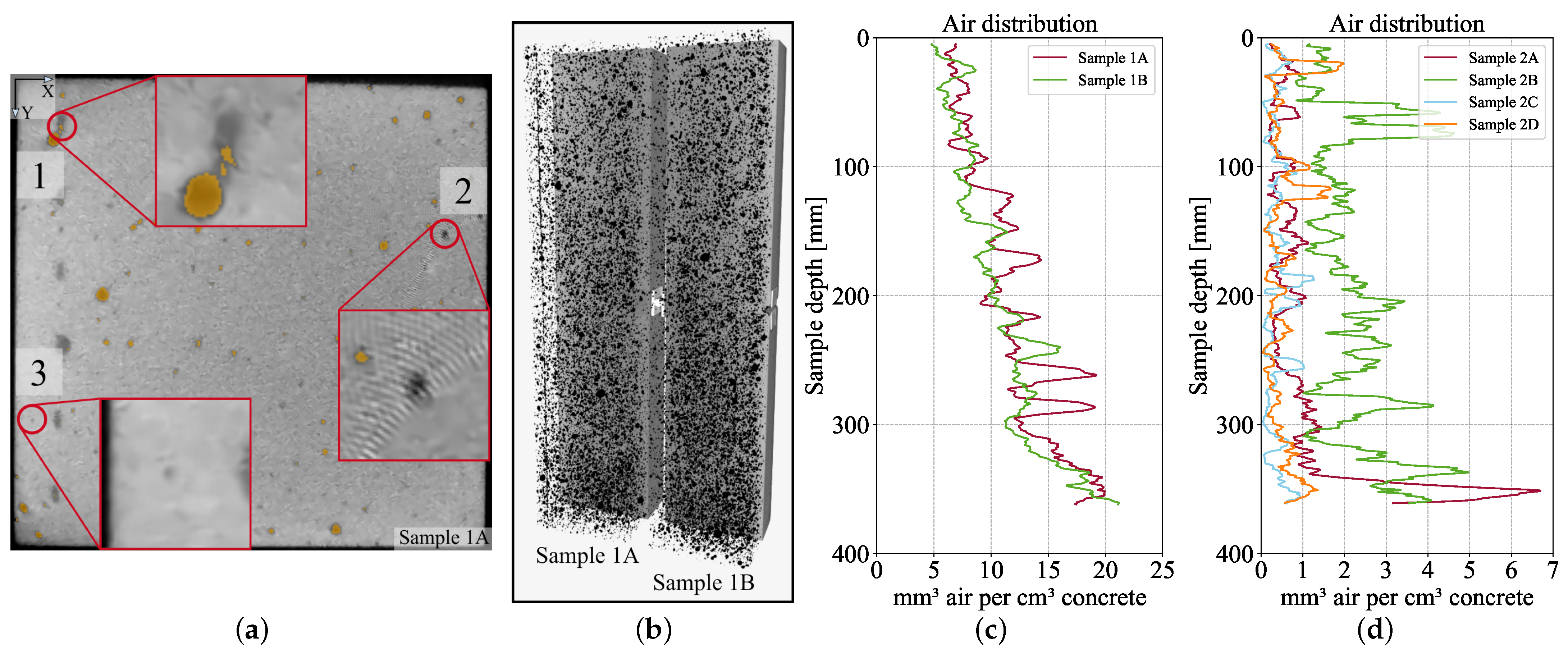
3.5.2. Porosity

To evaluate the concrete porosity, the first step was to segment the pores, using the 3D U-Net. This process used two trained versions: one using online augmentation and the other using offline augmentation, as described in [38]. Training was performed on two RTX A6000 GPUs, each with 48 GB of VRAM.

The offline augmentation strategy expanded the dataset from 8.3 GB to 39.9 GB, and the associated CNN was trained for 50 epochs, using 9 days and 6 h. Conversely, with online augmentation, the CNN was trained for 200 epochs in a much shorter time of 4 days and 20 h. The offline augmentation method achieved an F1 score of 88.22%, while the online augmentation approach yielded an F1 score of 86.44%. Therefore, the CNN trained on the offline augmented dataset was selected.

However, despite the satisfactory performance of the 3D U-Net model, the segmentation still showed imperfections, due to the augmentation strategies causing the CNN to falsely segment certain parts of the carbon (see Figure 21a). However, as segmentation was nearly perfect in areas where only concrete was present, the distribution calculation focused solely on these regions, to estimate concrete porosity.

On average, Sample 1A had a pore volume of 11.6 mm${}^3$ and Sample 1B had 10.6 mm${}^3$ of air per 1 cm${}^3$ of concrete. These values corresponded to porosities of 1.16 vol% and 1.06 vol%, respectively. Experiment 2, on the other hand, showed significantly fewer observed pores:

• Sample 2A: 0.9 mm${}^3$ air per cm${}^3$ concrete (porosity: 0.09 vol%);
• Sample 2B: 2.2 mm${}^3$ air per cm${}^3$ concrete (porosity: 0.22 vol%);
• Sample 2C: 0.4 mm${}^3$ air per cm${}^3$ concrete (porosity: 0.04 vol%);
• Sample 2D: 0.5 mm${}^3$ air per cm${}^3$ concrete (porosity: 0.05 vol%).

This phenomenon can be attributed to the application of some additional, vibrational compaction during the casting process for the samples of Experiment 2, in order to ensure the complete penetration of the close-meshed reinforcement cage while, concurrently, the release of air was facilitated. This process resulted in a quite low quantity but uniform distribution of air voids in the concrete matrix (Figure 21d). By contrast, the distribution of pores in Samples 1A and 1B (Figure 21c) revealed a different trend, which can be seen directly by a visual inspection of Figure 21b: The beams show a significantly higher concentration of pores at the bottom compared to the top. It can be concluded that the release of air voids that were entrapped closer to the bottom within the vertical formwork was impeded, due to the absence of additional compaction for these specimens.

However, while the compaction resulted in concrete with fewer pores in Experiment 2, it also introduced a specific limitation to their investigation. As the reduction of contained air voids led to poor texture of the CT data, not enough clearly identifiable points between two time steps could be found for the DVC method and, therefore, no analysis was possible. Note that the obtained distribution was expected to be much smaller than the real porosity, due to the large voxel size of 125.844 µm. Pores with a diameter of 1 to 2 voxels were not detectable, due to the noise (Section 2.4.1) and, thus, pores smaller than ≈0.25 mm could not be measured.

4. Discussion

This article investigates the development of cracks in CRC beams during in situ bending tests. Different measurement systems were used for the identification of the cracks as well as their characterization. Of particular interest were the non-destructive methods, which are becoming increasingly important in the construction industry. The present study highlights the use of computed tomography with high energy, which enables scanning specimen cross-sections up to 800 × 160 mm${}^2$. DVC as well as DIC methods for identifying cracks in large datasets were tested. In addition, an alternative procedure for measuring crack widths for non-structured and/or non-temporal CT data was proposed, as well as two application-related quality analyses. The following conclusions can be drawn from this study:

• The development of cracks in the middle section (the field of view of the CT and stereo camera system) of the CRC beams could be successfully observed. The complex characteristics of the crack geometry could be analyzed from various images in different load stages.
• Despite the high noise in the CT data, it was possible to apply DVC to detect cracks in the first experiment. By contrast, the texture in the second experiment was not adequate for the usage of DVC.
• A high-quality stereo camera system was applied, to observe the front surfaces of the specimens, to detect cracks and to measure their widths, which were compared to the results of the DVC. The RMSE as a measure of accuracy was 0.055 mm, which corresponds to 0.44 vx.
• In addition, an alternative voxel data analysis was performed, to measure crack widths, which can also be applied if the texture of the CT image data is not suitable for DVC or if no temporal data are available. For the first experiment, the resulting values systematically overestimated the values of the DVC. The corresponding large RMSE was 0.33 mm. The cracks seemed to be over-represented in the CT reconstruction data. Although the algorithm could not be tested on the second experiment, because the widths of the cracks were smaller than a voxel, it did not rely on the presence of structure in a reconstruction.
• In the processing of the 3D data, inspections of the manufacturing quality of the CRC beams could be carried out. In particular, the evaluation included measuring the distance of the reinforcement from the surface, to ensure the correct concrete cover thickness, and estimating the porosity.

5. Conclusions and Outlook

This publication presents voxel data analysis of bending tests observed by in situ X-ray tomography. Crack detection and the measurement of their widths were performed by applying digital volume correlation and, additionally, by gray value profile analysis. The formation of cracks could be observed at different stages of loading the beam. The resulting crack widths were compared and an overestimation of the latter method was determined. The DVC measurements were also benchmarked against the results from a digital image correlation system with a RMSE of 0.055 mm. Furthermore, it was shown how to analyze the CT data for quality control (estimation of the location of the reinforcement and its concrete cover as well as the porosity).

Future work could concentrate on possible adjustments that could be implemented in the CT device settings, to reduce noise in the CT measurement data. This could be done by using more appropriate radiation energies or by taking multiple images at each rotation step. Another approach to guaranteeing the generation of usable measurement data concerns the creation of a suitable texture through air voids or small additives with a distinguishable density compared to the concrete matrix.

References

- Peled, A.; Bentur, A.; Mobasher, B. Textile Reinforced Concrete, 1st ed.; CRC Press: Boca Raton, FL, USA, 2017. [Google Scholar] [CrossRef]
- Beckmann, B.; Adam, V.; Marx, S.; Chudoba, R.; Hegger, J.; Curbach, M. Novel Design Strategies for Material-Minimized Carbon Reinforced Concrete Structures—Overview of the Research in CRC/TRR 280. In Proceedings of the Building for the Future: Durable, Sustainable, Resilient; Ilki, A., Çavunt, D., Çavunt, Y.S., Eds.; Springer: Cham, Switzerland, 2023; pp. 1242–1251. [Google Scholar] [CrossRef]
- Brisard, S.; Serdar, M.; Monteiro, P.J. Multiscale X-ray tomography of cementitious materials: A review. Cem. Concr. Res. 2020, 128, 105824. [Google Scholar] [CrossRef]
- Schulze, S. Radiographie im Bauwesen–Einsatzmöglichkeiten in der Praxis im Rahmen der ZfPBau. Beton-und Stahlbetonbau 2022, 117, 1008–1017. [Google Scholar] [CrossRef]
- Skarźyński, Ł.; Suchorzewski, J. Mechanical and fracture properties of concrete reinforced with recycled and industrial steel fibers using Digital Image Correlation technique and X-ray micro computed tomography. Constr. Build. Mater. 2018, 183, 283–299. [Google Scholar] [CrossRef]
- du Plessis, A.; Boshoff, W.P. A review of X-ray computed tomography of concrete and asphalt construction materials. Constr. Build. Mater. 2019, 199, 637–651. [Google Scholar] [CrossRef]
- Bay, B.K.; Smith, T.S.; Fyhrie, D.P.; Saad, M. Digital Volume Correlation: Three-dimensional Strain Mapping Using X-ray Tomography. Exp. Mech. 1999, 39, 217–226. [Google Scholar] [CrossRef]
- Lorenzoni, R.; Curosu, I.; Léonard, F.; Paciornik, S.; Mechtcherine, V.; Silva, F.A.; Bruno, G. Combined mechanical and 3D-microstructural analysis of strain-hardening cement-based composites (SHCC) by in-situ X-ray microtomography. Cem. Concr. Res. 2020, 136, 106139. [Google Scholar] [CrossRef]
- Suleiman, A.R.; Zhang, L.V.; Nehdi, M.L. Quantifying Crack Self-Healing in Concrete with Superabsorbent Polymers under Varying Temperature and Relative Humidity. Sustainability 2021, 13, 13999. [Google Scholar] [CrossRef]
- Gökçe, H.; Öztürk, B.C.; Çam, N.; Andiç-Çakır, Ö. Gamma-ray attenuation coefficients and transmission thickness of high consistency heavyweight concrete containing mineral admixture. Cem. Concr. Compos. 2018, 92, 56–69. [Google Scholar] [CrossRef]
- Grzesiak, S.; Pahn, M.; Basters, R.; de Sousa, C. Application of the Computed Tomography in Structural Engineering. In Proceedings of the International Symposium of the International Federation for Structural Concrete; Springer: Cham, Switzerland, 2023; pp. 1903–1912. [Google Scholar] [CrossRef]
- Millner, M.R.; Payne, W.H.; Waggener, R.G.; McDavid, W.D.; Dennis, M.J.; Sank, V.J. Determination of effective energies in CT calibration. Med. Phys. 1978, 5, 543–545. [Google Scholar] [CrossRef]
- Giese, J.; Herbers, M.; Liebold, F.; Wagner, F.; Grzesiak, S.; Sousa, C.d.; Pahn, M.; Maas, H.G.; Marx, S.; Curbach, M.; et al. Investigation of the Crack Behavior of CRC Using 4D Computed Tomography, Photogrammetry and Fiber Optic Sensing. Buildings 2023, 13, 2595. [Google Scholar] [CrossRef]
- Wilhelm Kneitz Solutions in Textile. Data sheet of SITgrid040. 2020. Available online: https://solutions-in-textile.com/ (accessed on 4 September 2023).
- Action Composites. Data sheet of Carbon4ReBAR (C4R). 2020. Available online: https://www.action-composites.com/carbon4rebar/ (accessed on 4 September 2023).
- Noo, F.; Defrise, M.; Clackdoyle, R.; Kudo, H. Image reconstruction from fan-beam projections on less than a short scan. Phys. Med. Biol. 2002, 47, 2525. [Google Scholar] [CrossRef]
- Jesse, F.; Kutzner, T. Digitale Photogrammetrie in der Bautechnik: Einfluss wichtiger Systemparameter und Genauigkeitspotenzial in der Praxis. Bautechnik 2013, 90, 703–714. [Google Scholar] [CrossRef]
- Sutton, M.A.; Orteu, J.J.; Schreier, H. Image Correlation for Shape, Motion and Deformation Measurements: Basic Concepts, Theory and Applications, 1st ed.; Springer: Cham, Switzerland, 2009. [Google Scholar] [CrossRef]
- Liebold, F.; Maas, H.G.; Deutsch, J. Photogrammetric determination of 3D crack opening vectors from 3D displacement fields. ISPRS J. Photogramm. Remote Sens. 2020, 164, 1–10. [Google Scholar] [CrossRef]
- Geers, M.G.D.; De Borst, R.; Brekelmans, W.A.M. Computing strain fields from discrete displacement fields in 2D-solids. Int. J. Solids Struct. 1996, 33, 4293–4307. [Google Scholar] [CrossRef]
- Liebold, F.; Maas, H.G. 3D-Deformationsanalyse und Rissdetektion in multitemporalen Voxeldaten von Röntgentomographen. In Proceedings of the Tagungsband der Dreiländertagung der DGPF, OVG und SGPF Photogrammetrie—Fernerkundung—Geoinformation—2022, Dresden, Germany, 5–6 October 2022; Volume 30, pp. 105–116. [Google Scholar] [CrossRef]
- Liebold, F.; Maas, H.G. Computational Optimization of the 3D Least-Squares Matching Algorithm by Direct Calculation of Normal Equations. Tomography 2022, 8, 760–777. [Google Scholar] [CrossRef]
- Dare, P.; Hanley, H.; Fraser, C.; Riedel, B.; Niemeier, W. An Operational Application of Automatic Feature Extraction: The Measurement of Cracks in Concrete Structures. Photogramm. Rec. 2002, 17, 453–464. [Google Scholar] [CrossRef]
- Benz, C.; Rodehorst, V. Model-based Crack Width Estimation using Rectangle Transform. In Proceedings of the 2021 17th International Conference on Machine Vision and Applications (MVA), Online, 25–27 July 2021; pp. 1–5. [Google Scholar] [CrossRef]
- Carrasco, M.; Araya-Letelier, G.; Velázquez, R.; Visconti, P. Image-Based Automated Width Measurement of Surface Cracking. Sensors 2021, 21, 7534. [Google Scholar] [CrossRef]
- Barisin, T.; Jung, C.; Müsebeck, F.; Redenbach, C.; Schladitz, K. Methods for segmenting cracks in 3d images of concrete: A comparison based on semi-synthetic images. Pattern Recognit. 2022, 129, 108747. [Google Scholar] [CrossRef]
- Terol-Villalobos, I.R. Morphological image enhancement and segmentation. Adv. Imaging Electron Phys. 2001, 118, 207–273. [Google Scholar] [CrossRef]
- Vicente, M.A.; González, D.C.; Mínguez, J. Recent advances in the use of computed tomography in concrete technology and other engineering fields. Micron 2019, 118, 22–34. [Google Scholar] [CrossRef]
- Khormani, M.; Jaari, V.R.K.; Aghayan, I.; Ghaderi, S.H.; Ahmadyfard, A. Compressive strength determination of concrete specimens using X-ray computed tomography and finite element method. Constr. Build. Mater. 2020, 256, 119427. [Google Scholar] [CrossRef]
- DIN EN 1992-1-1:2011-01; Eurocode 2 Design of Concrete Structures—Part 1-1: General Rules and Rules for Buildings; German version EN 1992-1-1:2004 + AC:2010. Deutsches Institut für Normung e.V.: Berlin, Germany, 2011.
- Deutscher Ausschuss für Stahlbeton. DAfStb-Richtlinie Betonbauteile mit nichtmetallischer Bewehrung; Draft Guideline; Deutscher Ausschuss für Stahlbeton: Berlin, Germany, 2022. [Google Scholar]
- Kalthoff, M.; Raupach, M.; Matschei, T. Investigation into the Integration of Impregnated Glass and Carbon Textiles in a Laboratory Mortar Extruder (LabMorTex). Materials 2021, 14, 7406. [Google Scholar] [CrossRef] [PubMed]
- Alsayed, S.H.; Amjad, M.A. Strength, Water Absorption and Porosity of Concrete Incorporating Natural and Crushed Aggregate. J. King Saud Univ.-Eng. Sci. 1996, 8, 109–119. [Google Scholar] [CrossRef]
- Claisse, P.A.; Cabrera, J.G.; Hunt, D.N. Measurement of porosity as a predictor of the durability performance of concrete with and without condensed silica fume. Adv. Cem. Res. 2001, 13, 165–174. [Google Scholar] [CrossRef]
- Schukraft, J.; Lohr, C.; Weidenmann, K.A. Approaches to X-ray CT Evaluation of In-Situ Experiments on Damage Evolution in an Interpenetrating Metal-Ceramic Composite with Residual Porosity. Appl. Compos. Mater. 2023, 30, 815–831. [Google Scholar] [CrossRef]
- Çiçek, Ö.; Abdulkadir, A.; Lienkamp, S.S.; Brox, T.; Ronneberger, O. 3D U-Net: Learning Dense Volumetric Segmentation from Sparse Annotation. In Proceedings of the Medical Image Computing and Computer-Assisted Intervention—MICCAI 2016; Ourselin, S., Joskowicz, L., Sabuncu, M.R., Unal, G., Wells, W., Eds.; Springer: Cham, Switzerland, 2016; pp. 424–432. [Google Scholar] [CrossRef]
- Wagner, F.; Maas, H.G. A Comparative Study of Deep Architectures for Voxel Segmentation in Volume Images. Int. Arch. Photogramm. Remote Sens. Spatial Inf. Sci. 2023, in press.
- Wagner, F.; Mester, L.; Klinkel, S.; Maas, H.G. Analysis of Thin Carbon Reinforced Concrete Structures through Microtomography and Machine Learning. Buildings 2023, 13, 2399. [Google Scholar] [CrossRef]
- Taha, A.A.; Hanbury, A. Metrics for evaluating 3D medical image segmentation: Analysis, selection, and tool. BMC Med. Imaging 2015, 15, 29. [Google Scholar] [CrossRef]