
Three-Dimensional Numerical Analysis on the Influence of Buttress Wall Removal Timing on the Lateral Deformation of Diaphragm Walls during Deep Excavation


Abstract
:1. Introduction
1.1. Literature Review

| Author | Abstract |
|---|---|
| Manna and Clough [8] | They utilized the finite element method to analyze factors influencing the deformation of excavation retaining walls. When comparing their findings with field observations from deep excavations, they identified several key influencing factors: the safety factor against uplift, stiffness of the retaining wall and support system, pre-stress magnitude of supports, plan geometry of the excavation area, and project duration. |
| Ou et al. [9] | They examined ten cases of deep excavation in the Taipei Basin where either pre-bored piles or diaphragm walls were employed. Their findings indicated that lateral displacements increased with excavation depth. The maximum lateral displacement (δh, max) ranged between 0.2% and 0.5% of the final excavation depth (He). Notably, in soft clays, the maximum displacement tends towards the upper limit, while in sandy grounds it leans towards the lower limit. |
| Clough and O’Rourke [10] | The patterns of retaining wall deformation due to excavation with internal struts and tie-backs can be categorized into cantilever displacement, deep inward displacement, and a combination of the two. Their analysis across different soil types—stiff clay, residual soil, and sand—revealed that the average maximum surface settlement was about 0.15 times the excavation depth. Cases with lateral displacement exceeding 0.5% of the excavation depth were attributed to construction malpractice or insufficient wall penetration. |
| Masuda et al. [11] | They categorized influential factors affecting excavation performance into two main groups based on an analysis of 52 excavation cases: soil stiffness and support stiffness. Furthermore, they summarized 11 reasons affecting retaining wall deformation, such as soil type, soil properties, wall stiffness, support quantity and spacing, pre-stress on supports, excavation method, wall length, ground improvement presence, scale of excavation, groundwater conditions, and other construction activities. |
| Wu et al. [12] | They consolidated data from Taipei’s metro construction and past excavation projects in the city. Their results showed a relationship between the maximum lateral wall displacement (δmax) and excavation depth (D) as δmax = (0.07% to 0.2%) D. The depth at which this maximum displacement occurs, Za, was related to the excavation depth as Za = (0.8 to 1.2) D, averaging around the excavation depth. |
| Wang et al. [13] | They analyzed deep excavation cases in Kaohsiung’s clay layer. Their findings suggested a relationship between the maximum lateral wall displacement (δh,max) and the excavation depth (H) as δh,max = (0.1% to 0.4%) H. |
| Surarak et al. [14] | They back-calculated the Eu/Su ratio using the MC model, providing a reliable prediction for the lateral movement of retaining walls. However, this model was less successful in predicting surface settlements. Utilizing soil parameters from lab and field tests for both SSM (Small Strain Model) and HSM (Hardening Soil Model) analyses led to improved agreement with observed lateral wall movements and surface settlements. |
| Hsieh et al. [2] | They proposed a simplified method for predicting wall displacement and designing diaphragm walls to ensure safety standards are met. They used a three-dimensional numerical analysis to study the factors influencing wall displacement during excavation. These factors encompass excavation geometry, diaphragm wall thickness, wall spacing, wall penetration depth, diaphragm wall stiffness, strut axial stiffness, diaphragm wall axial stiffness, and undrained shear strength of clay. |
| Author | Abstract |
|---|---|
| Peck [15] | He compiled observational data on ground subsidence from excavation cases in areas such as Chicago and Oslo, proposing a relationship between ground subsidence (δv) and distance from the retaining wall (d). |
| Ou and colleagues [9,16,17] | They delineated that subsidence from deep excavation generally exhibits two patterns: triangular trough and concave trough. |
| Wang et al. [13] | They analyzed deep excavation cases in Kaohsiung, concluding that the relationship between maximum ground subsidence and excavation depth is approximately δv,max = (0.04–0.25%)He, where He is excavation depth and δv,max = (0.21–1.10) δv,max for maximum wall displacement. |
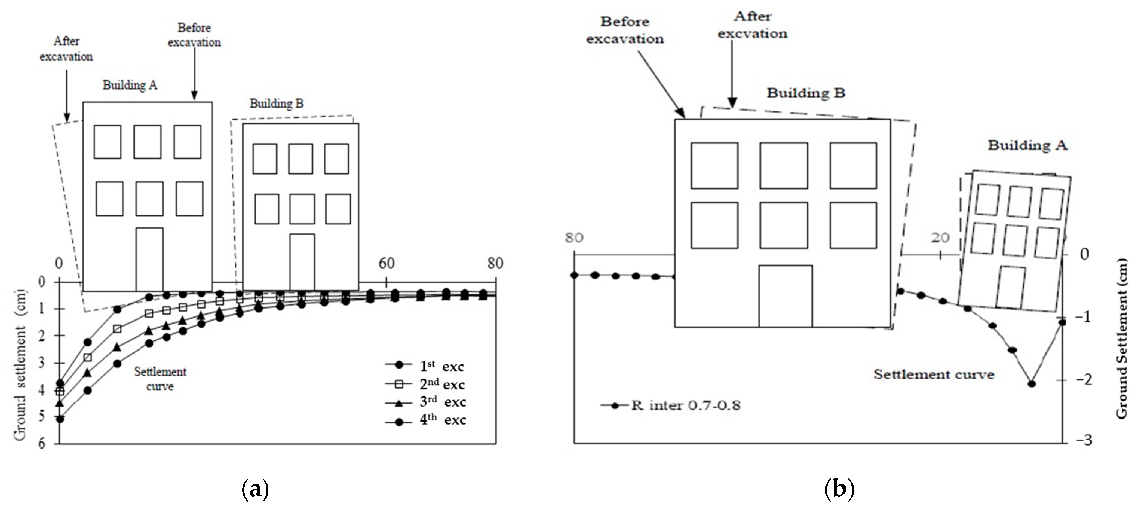
| Avanti [18] | He observed that the finite element analysis of ground subsidence in the Jakarta Metro project shows an arch-shoulder type. Larger Rinter values (as a parameter to represent interfaces between soil and structure) lead to a concave trough type of ground subsidence, which accurately predicts building damage, as illustrated in Figure 1a. If the subsidence is of the concave type, taking the TNEC (Taipei National Enterprise Center) case as an example (Ou [19]), it can be discerned from the ground subsidence contour that Building A has tilted and begun to sink during excavation, as shown in Figure 1b. |
| Author | Abstract |
|---|---|
| Liao [20], Wang [21] and Hsieh [22] | They utilized numerical analysis to study the behavior of wall deformation and ground subsidence in Taipei’s deep excavation projects. The results indicated a significant underestimation of maximum ground subsidence (δv,max), which often appeared further from the retaining wall than the actual observations. This led to overestimations in secondary affected areas, and unconverged values at the end of these regions. The primary reason for these discrepancies was that the existing analysis could not smoothly simulate the small strain behavior of the soil. |
| Hsieh [23] and others | They pointed out that three-dimensional numerical analysis simulating excavations in Taipei with central walls and struts compared well with monitoring data. |
| Chen et al. [24] | They used a 3D software tool to study the effect of exterior struts in reducing the maximum lateral deformation in the middle of the Diaphragm Wall. |
| Khoiri and Ou [25] | They explored wall displacement and ground subsidence for the Kaohsiung Metro System O6 station using both MC (Mohr-Coulomb Model) and HS (Hardening Soil Model). |
| Ou et al. [26] | They showed that installing a central wall can reduce the maximum wall deformation by 75% and maximum ground subsidence by 82%. They discussed the corner effects of retaining walls using a 3D numerical method. |
| Ye [27] | They used PLAXIS 3D Foundation to simulate a real project, suggesting that central walls and struts can significantly enhance the stiffness of the Diaphragm Wall. |
| Feng [28] | They employed the “Plaxis 3D” software to study the effects of different spacings, thicknesses, and penetration depths for struts and central walls, emphasizing their effectiveness in reducing lateral wall movement and ground subsidence. |
1.2. Introduction to Buttress Walls, Cross Walls, and Wall Piles
- Internal Buttress Walls: Positioned on the excavation side of the diaphragm wall, these walls primarily serve to enhance the wall’s rigidity, curbing deformations due to excavation-induced decompression. They are progressively removed as excavation proceeds and can be regarded as a temporary support system.
- External Buttress Walls: Located on the non-excavated side of the diaphragm wall, external Buttress Walls differ from their internal counterparts. They are seen as an integral part of the diaphragm wall structure and are usually reinforced. Their primary function is to increase the rigidity of the diaphragm wall. Unlike internal walls, they are not removed during excavation phases.
- Cross Walls: These walls are set up to connect the Diaphragm Wall on either the north-south or east-west sides and can be seen as a support system. They offer significant rigidity to the diaphragm walls, effectively limiting wall deformation, differential foundation settlement, and providing resistance against uplift. They are generally reinforced below the excavation face and are removed progressively with excavation.
- Wall Piles: A subset of foundation piles, wall piles play a vital role in preventing uplift, enhancing foundational load-bearing capacity, and minimizing differential settlement.
2. Materials and Methods
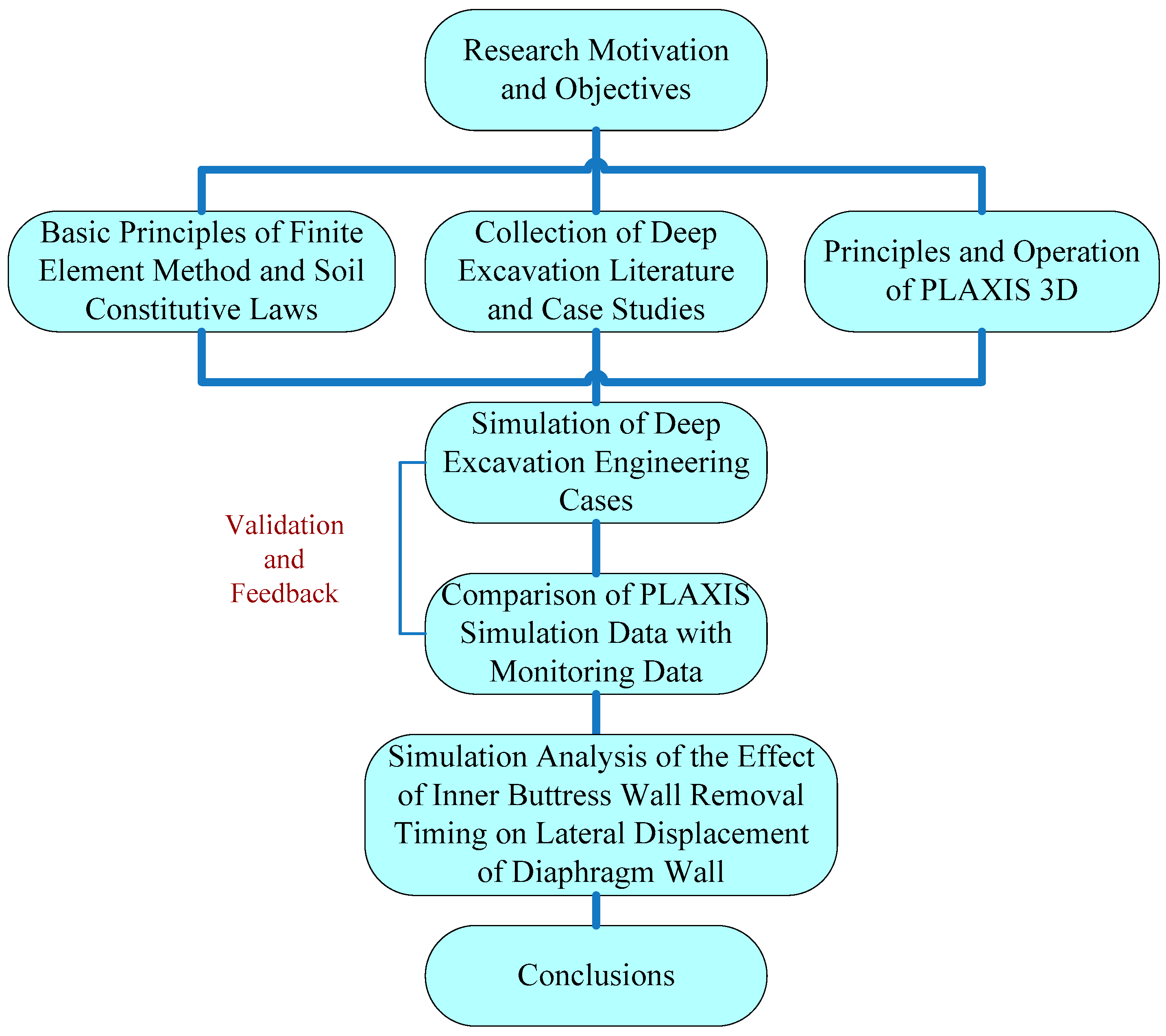
2.1. Research Methodology and Steps
2.2. Research Content
- Validation of PLAXIS Numerical Analysis Simulation and Monitoring Data
- Simulation Analysis of the Timing for Internal Buttress Wall Removal
2.3. Numerical Simulation
- (1)
- Software Overview
- Simulation capabilities encompassing: elements, soil bodies, various elements and soil body interfaces, wall, plate, beam structures, pile foundations, braces and anchors, tunnels, and groundwater seepage analysis.
- Analytical capability for deformation, consolidation, graded loading, stability, and seepage, as well as variations in shear, bending moment, and axial stress for various structures, hydrosols, and temporary support elements. It can also consider the impact of low-frequency seismic loads.
- In terms of soil material stress-strain constitutive models, it offers:
- Linear-elasticity model.
- Mohr-Coulomb model.
- Soft Soil Creep Model.
- Hardening Soil Model.
- Hardening Soil Model with Small-strain.
- (2)
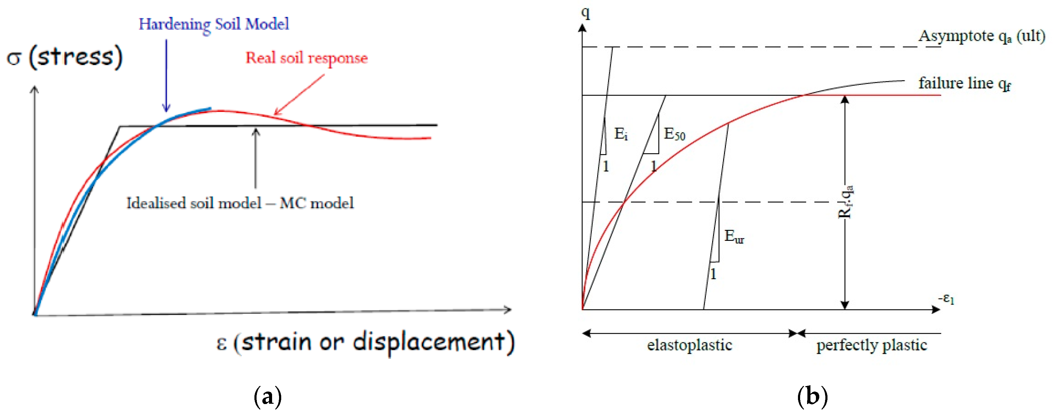
- Hardening Soil Model
- Principles
- Input Parameters for the HS Model
- 1.
- General ParametersSaturated unit weight γsat and unsaturated unit weight γunsat (kN/m3), along with the porosity ratio e.
- 2.
- Stiffness Parameters: Triaxial drained secant modulus under reference stress.: One-dimensional oedometric secant modulus under reference stress.: Modulus of elasticity for loading-unloading under reference stress.m: Power for the relation between elastic modulus and stress.
- 3.
- Strength ParametersCref: Effective cohesionφ: Effective friction angle (deg)Ψ: Dilation angle (deg)
- 4.
- Advanced Strength Parameters: Poisson’s ratio for unloading-reloading. By default in the PLAXIS 3D manual, it is 0.2.pref: Reference stress. According to the PLAXIS 3D manual, the default is 100 stress units.Rf : Failure ratio. By default in the PLAXIS 3D manual, it is set to 0.9.: Tensile strength. The default value is 0 (kN/m2).
2.4. Parameter Settings for Soil Layer Drainage Conditions
- Drained Conditions
- Undrained (A) Parameters
- Undrained (B) Parameters
- Undrained (C) Parameters
- Non-Porous Condition
2.5. Model Creation Process
- Define the overall boundary profile of the model.
- Specify the soil parameters.
- Structure simulation.
- Adjacent building load simulation.
- Define construction steps and water level settings.
- Specify the mesh and mesh density.
2.6. Model Limitations
- Element Number Limitations:
- -
- Complexity: PLAXIS has a limit on the number of elements that can be modeled. For highly complex structures or extensive geotechnical scenarios, this could be a limiting factor.
- -
- Computational Efficiency: More elements mean longer computation times and more intensive use of computer resources.
- Material Properties:
- -
- Accuracy: There are limits in modeling the exact material properties, especially for heterogeneous soil conditions or complex materials.
- -
- Non-linearity: Although PLAXIS can handle non-linear materials, there can be complexities and limitations in extreme scenarios.
- Boundary Conditions:
- -
- Flexibility: While PLAXIS offers a range of options for setting boundary conditions, in some specialized or extreme cases, the options might not be adequate.
- -
- Real-World Representations: Representing real-world boundary conditions accurately can sometimes be challenging.
- Loading Conditions:
- -
- Dynamic Loads: There might be limitations in simulating certain types of dynamic or cyclic loading conditions.
- -
- Extreme Loads: While PLAXIS is capable of simulating a variety of load types, extreme loading scenarios can sometimes push beyond its capabilities.
- Analysis Types:
- -
- Consolidation Analysis: PLAXIS has certain constraints in dealing with very long-term consolidation and creep analysis.
- -
- Environmental Factors: The simulation of some specific environmental influences might be constrained.
- Software and Hardware Interaction:
- -
- Hardware Limitations: The performance of PLAXIS is also dependent on the hardware on which it is run. Hence, limitations in hardware can impact the efficiency and speed of analysis.
- -
- Parallel Processing: There could be limitations in the efficiency of parallel processing for very large models or complex analyses.
3. Numerical Simulation and Monitoring Data Validation
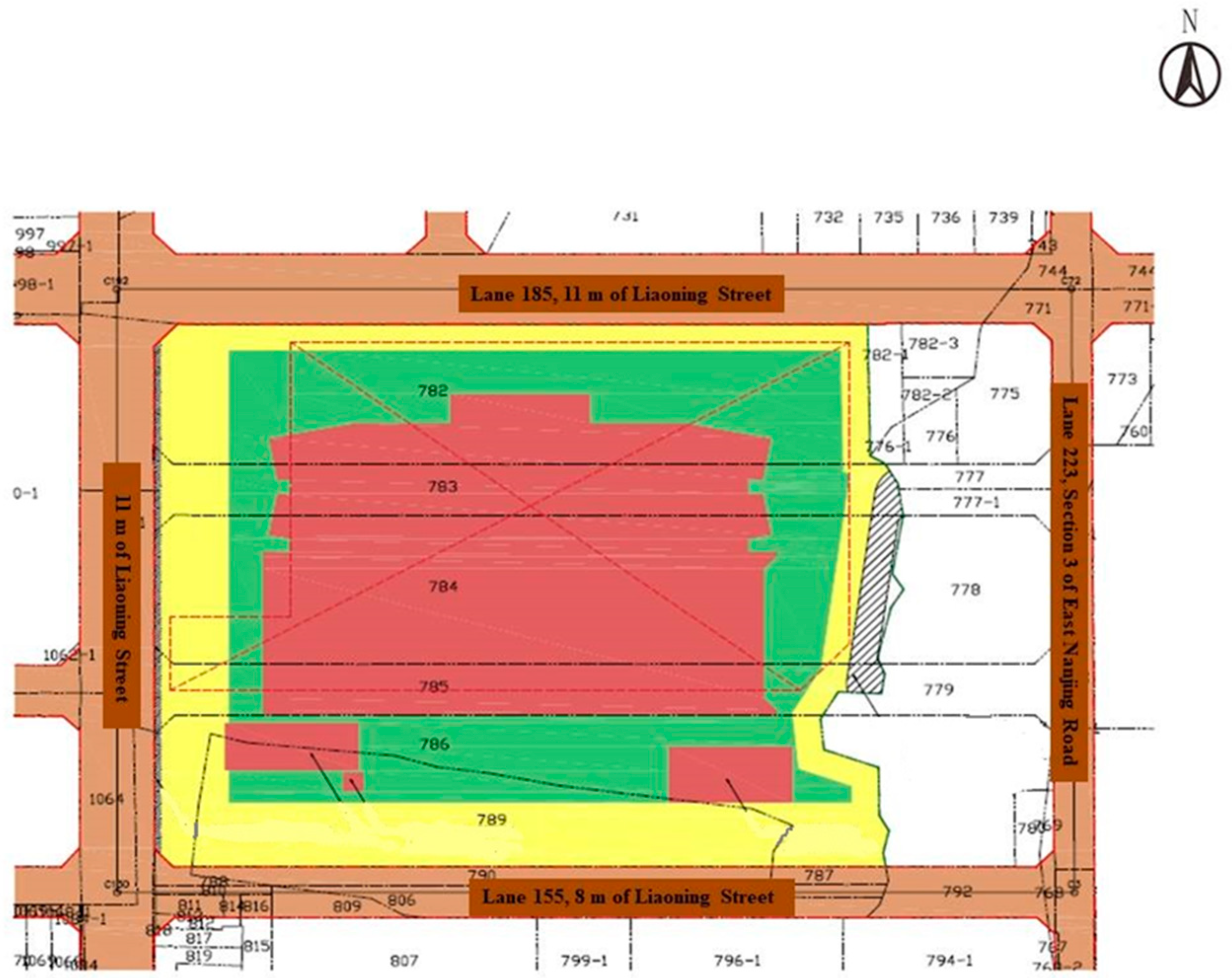
3.1. Case Overview
- (1)
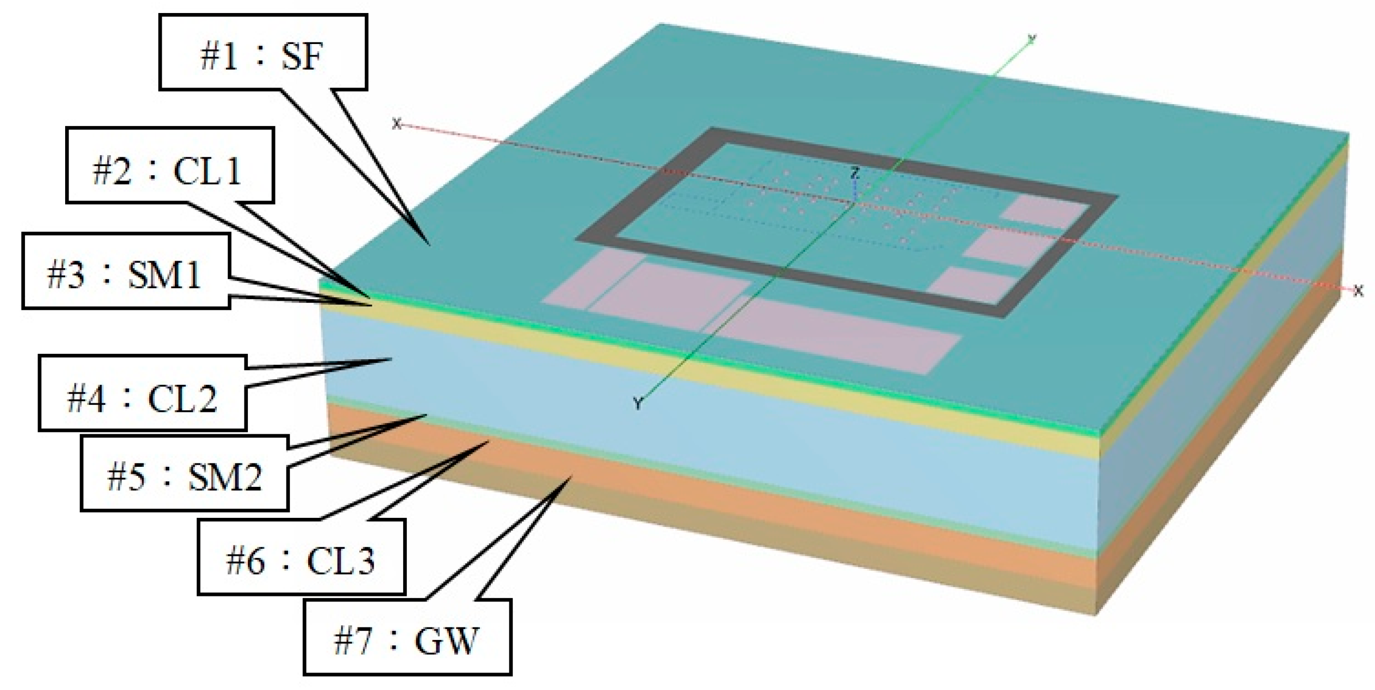
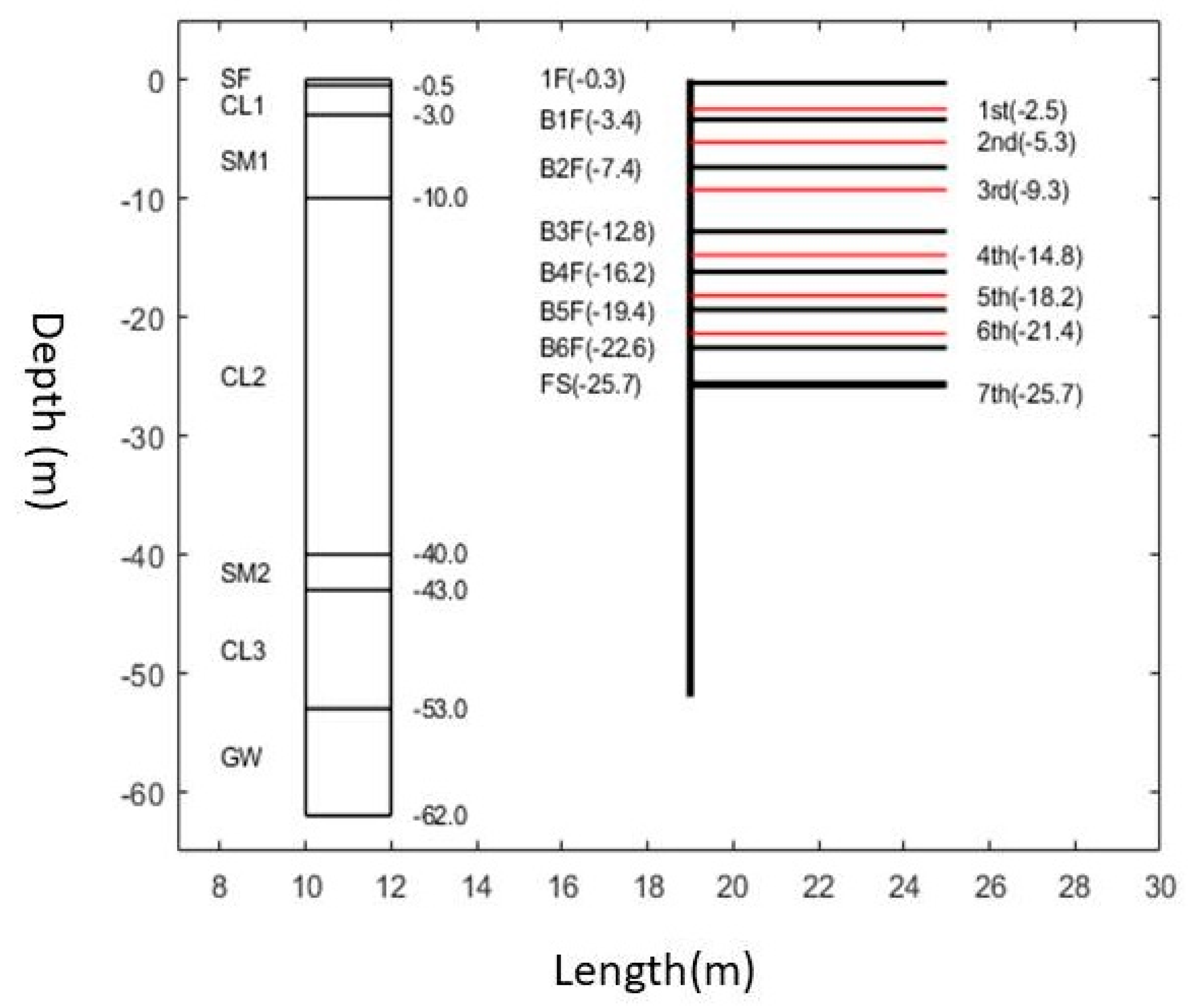
- Stratigraphy Overview
- (2)
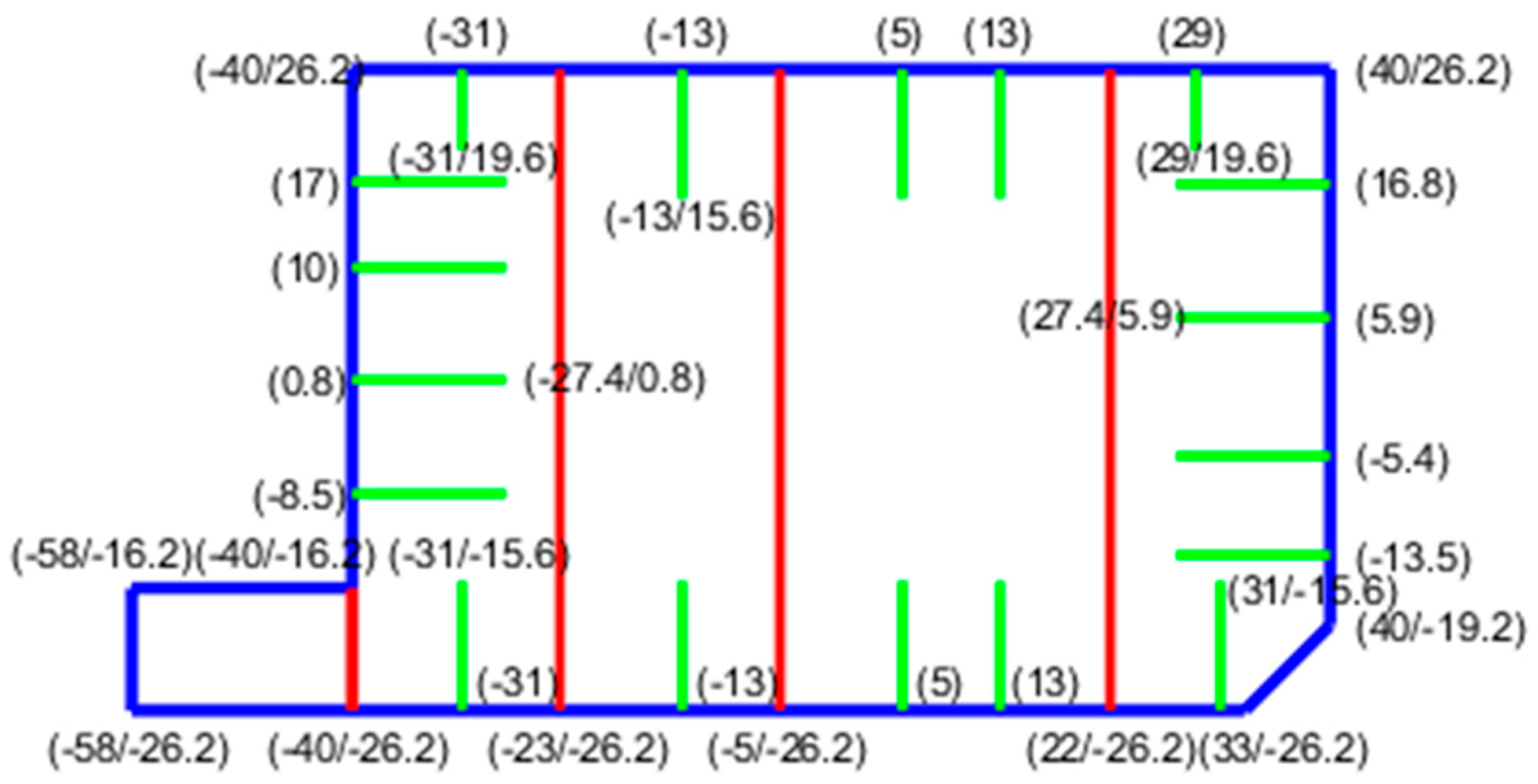
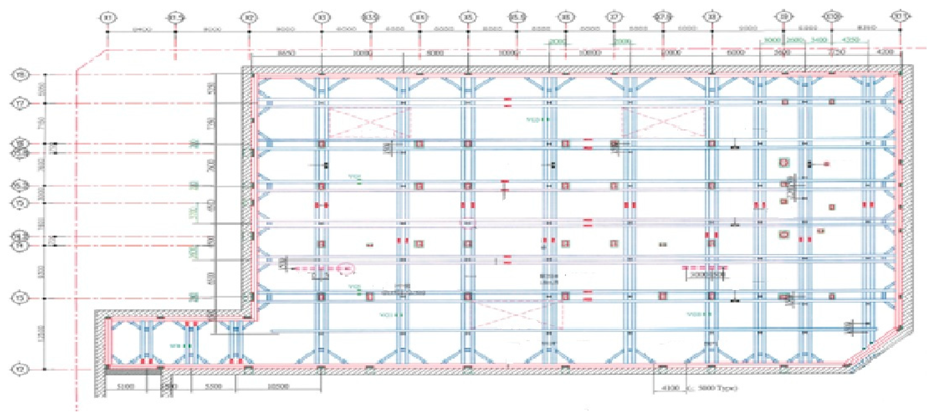
- Diaphragm Wall, Buttress Wall, and Cross Wall Overview
- (3)
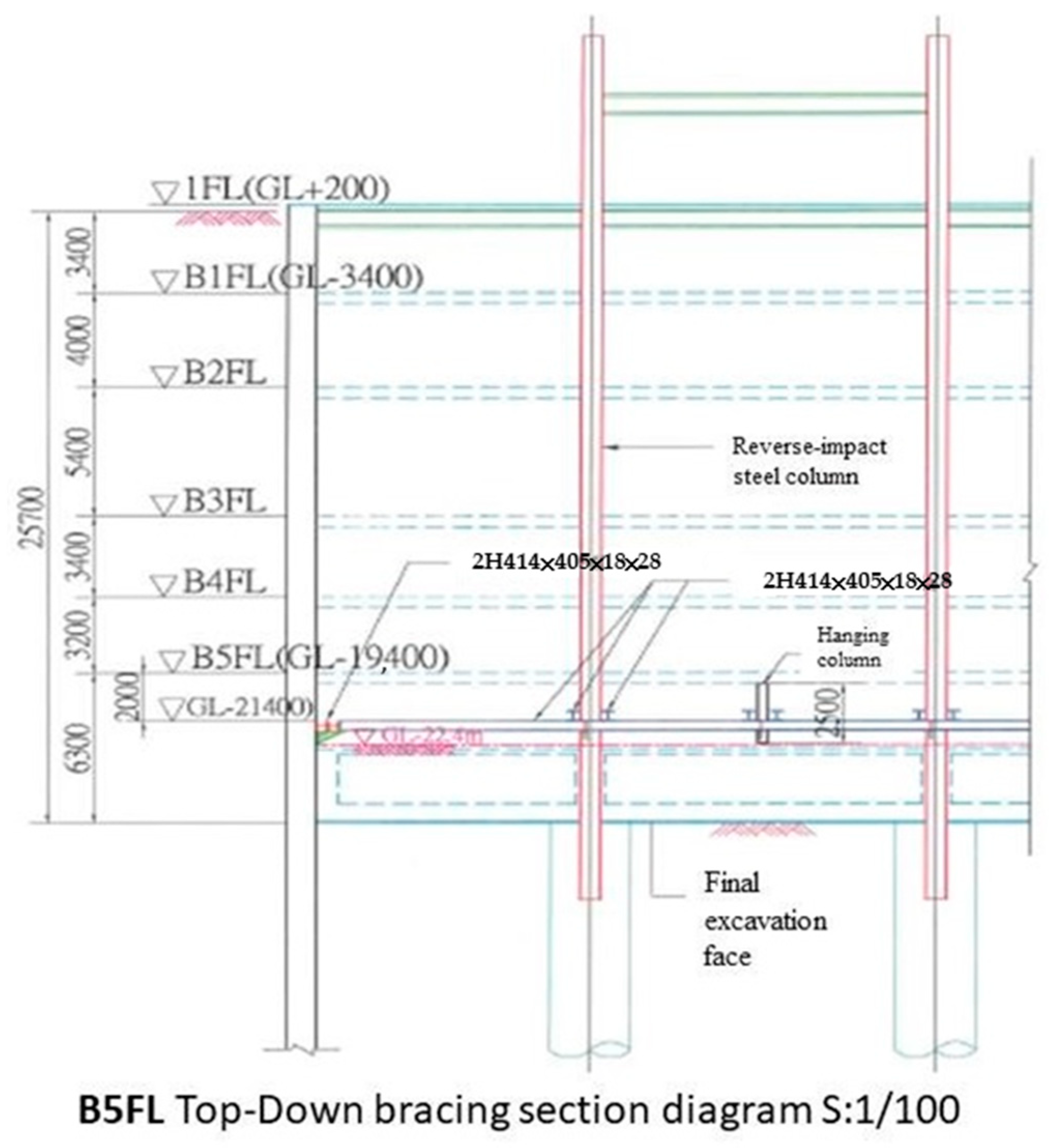
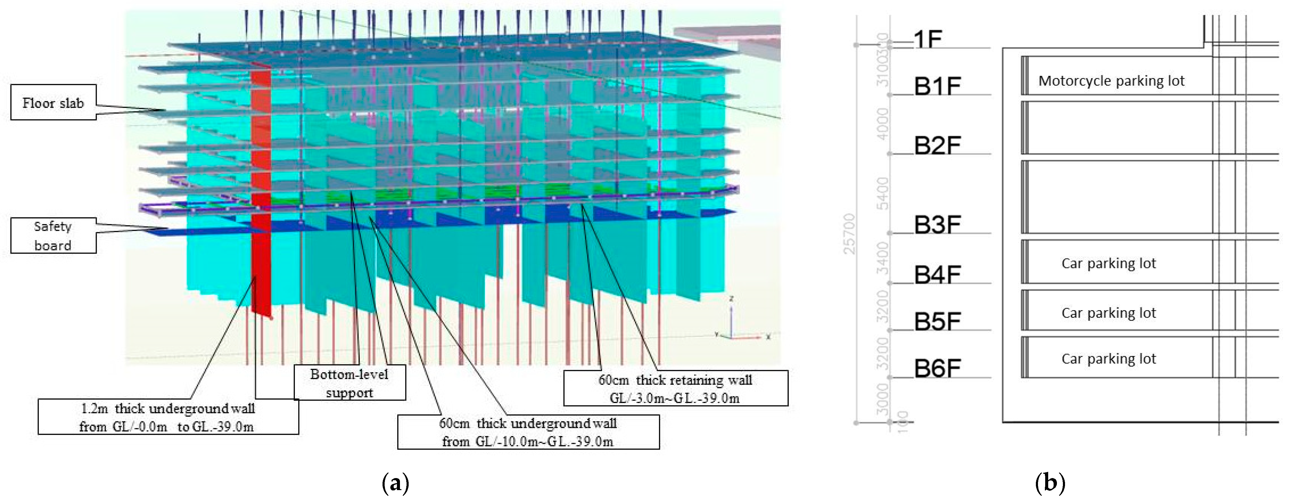
- Overview of the Top-down Construction Method
- (4)
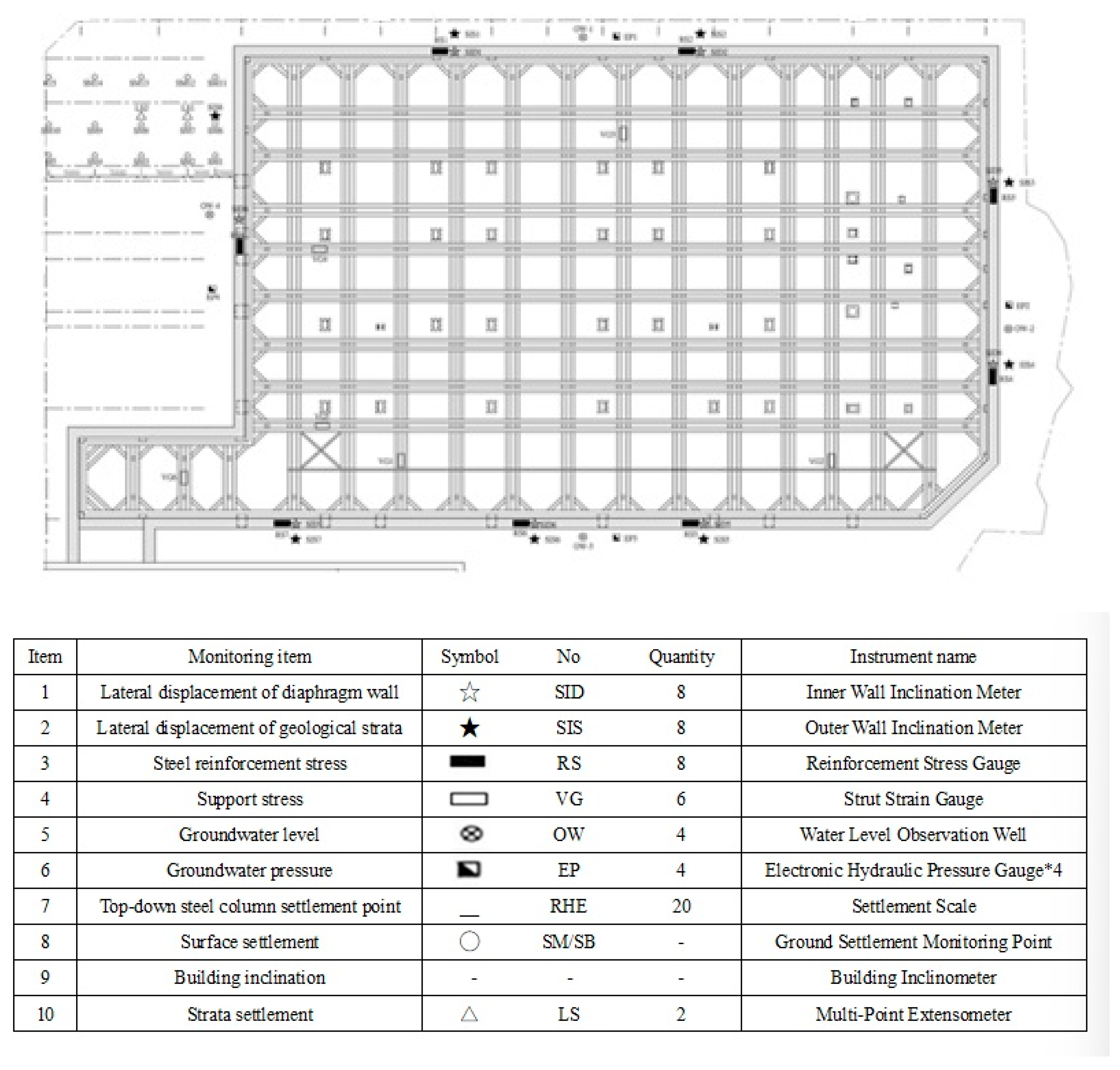
- Introduction to the Monitoring System
3.2. Case Study Simulation
- (1)
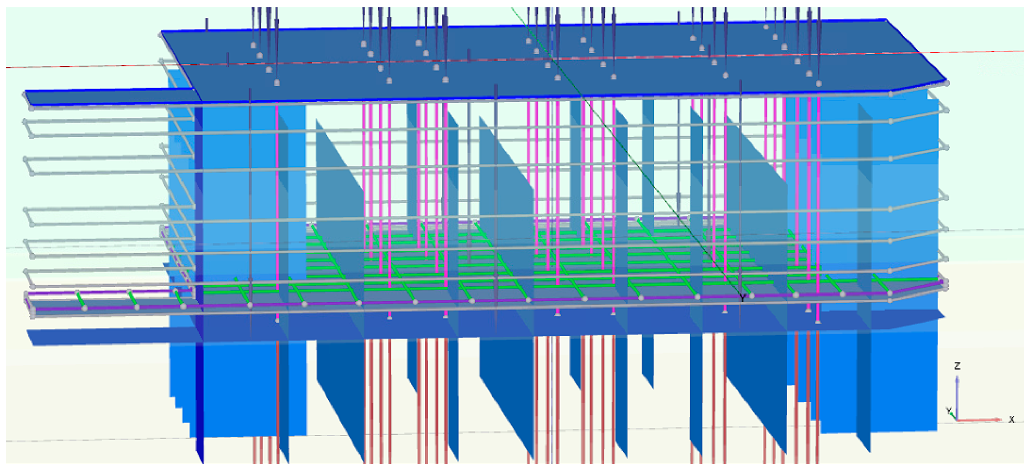
- Model Geometry
- (2)
- Initial Soil Stress
- (3)
- Soil Parameter Selection
- (4)
- Setting of Neighboring Building and Road Load Parameters
- (5)
- Parameters for Diaphragm Wall, Buttress Wall, Cross Wall, Floor Slabs, and Foundation Slab
- (6)
- Pile Wall Parameter Configuration
- (7)
- Top-Down Construction Steel Column Parameter Configuration
- (8)
- Bracing Parameter Configuration
3.3. Construction Steps
- (1)
- Initial phase: Establishment of initial ground stresses.
- (2)
- Phase 1:
- Load application from adjacent buildings and roads.
- Construction of diaphragm walls, cross walls, buttress walls, wall piles, and top-down steel columns, followed by zeroing displacements.
- (3)
- Phase 2:
- First excavation to GL.−2.5 m, concurrently demolishing the metro exit cross wall to GL.−2.5 m.
- Dewatering corresponding with the excavation depth.
- Construction of 1F floor slab at GL.−0.3 m.
- (4)
- Phase 3:
- Second excavation to GL.−5.3 m, with simultaneous removal of the buttress walls and metro exit cross wall to that depth.
- Corresponding dewatering.
- B1F floor slab establishment at GL.−3.4 m.
- (5)
- Phase 4:
- Third excavation to GL.−9.3 m, with parallel demolition of the buttress walls and metro exit cross wall.
- Dewatering as per excavation.
- B2F floor construction at GL.−7.4 m.
- (6)
- Phase 5:
- Fourth excavation to GL.−14.8 m, with concurrent demolition activities.
- Relevant dewatering.
- B3F floor establishment at GL.−12.8 m.
- (7)
- Phase 6:
- Fifth excavation to GL.−18.2 m, with simultaneous demolition tasks.
- Dewatering in line with excavation.
- B4F floor construction at GL.−16.2 m.
- (8)
- Phase 7:
- Sixth excavation to GL.−21.4 m, alongside demolition activities.
- Associated dewatering.
- B5F floor establishment at GL.−19.4 m.
- (9)
- Phase 8:
- Seventh excavation to GL.−22.6 m, in parallel with demolition.
- Corresponding dewatering.
- Horizontal bracing installation at GL.−21.8 m.
- (10)
- Phase 9:
- Eighth excavation reaching GL.−25.7 m, alongside the usual demolition tasks.
- Dewatering to match excavation.
- Foundation slab (FS) construction at GL.−25.7 m and B6 floor slab at GL.−22.6 m.
- Removal of the horizontal bracing at GL.−21.8 m.
3.4. Analysis Results and Model Validation
- Lateral Displacement Analysis and Comparison:
- 2.
- Settlement Analysis and Comparison:
4. Simulation Analysis of Timing for Removing Buttress Walls
4.1. Simulation Steps
- (1)
- Initial Phase: Establishment of the initial geotechnical conditions.
- (2)
- Phase 1:
- Establishment of loadings from adjacent buildings and roads.
- Construction of Diaphragm Wall, cross walls, buttress walls, wall piles, and top-down steel columns, followed by resetting displacements to zero.
- (3)
- Phase 2:
- First excavation to GL.−2.5 m while simultaneously demolishing the subway exit cross walls down to GL.−2.5 m.
- Dewatering in coordination with the excavation to GL.−2.5 m.
- Construction of the 1F floor slab at GL.−0.3 m.
- (4)
- Phase 3:
- Second excavation to GL.−5.3 m, accompanied by the demolition of the buttress walls and subway exit cross walls down to GL.−5.3 m.
- Dewatering in sync with the excavation to GL.−5.3 m.
- Construction of the B1F floor slab at GL.−3.4 m.
- (5)
- Phase 4:
- Third excavation to GL.−9.3 m, concurrently demolishing the buttress walls and subway exit buttress walls down to GL.−9.3 m.
- Dewatering in tandem with the excavation to GL.−9.3 m.
- Construction of the B2F floor slab at GL.−7.4 m.
- (6)
- Phase 5:
- Fourth excavation to GL.−14.8 m, while simultaneously removing the buttress walls, cross walls, and subway exit buttress walls down to GL.−14.8 m, with a gradual demolition of the southern buttress walls.
- Dewatering in alignment with the excavation to GL.−14.8 m.
- Construction of the B3F floor slab at GL.−12.8 m.
- (7)
- Phase 6:
- Fifth excavation to GL.−18.2 m, coinciding with the demolition of the buttress walls, cross walls, and subway exit buttress walls down to GL.−18.2 m.
- Dewatering alongside the excavation to GL.−18.2 m.
- Construction of the B4F floor slab at GL.−16.2 m.
- (8)
- Phase 7:
- Sixth excavation to GL.−21.4 m, in conjunction with the removal of the retaining walls, cross walls, and subway exit buttress walls down to GL.−21.4 m.
- Dewatering congruent with the excavation to GL.−21.4 m.
- Construction of the B5F floor slab at GL.−19.4 m.
- (9)
- Phase 8:
- Seventh excavation to GL.−22.6 m, simultaneous to the demolition of the retaining walls, cross walls, and subway exit buttress walls down to GL.−22.6 m.
- Dewatering in parallel with the excavation to GL.−22.6 m.
- Installation of horizontal bracing at GL.−21.8 m.
- (10)
- Phase 9:
- Eighth excavation to GL.−25.7 m, accompanied by the removal of the retaining walls, cross walls, and subway exit buttress walls down to GL.−25.7 m, plus the demolition of the previously gradually removed southern buttress walls at B3F.
- Dewatering coordinated with the excavation to GL.−25.7 m.
- Construction of the foundation slab (FS) at GL.−25.7 m; Construction of the B6 floor slab at GL.−22.6 m.
- Dismantling of the horizontal bracing at GL.−21.8 m.
4.2. Analysis Results
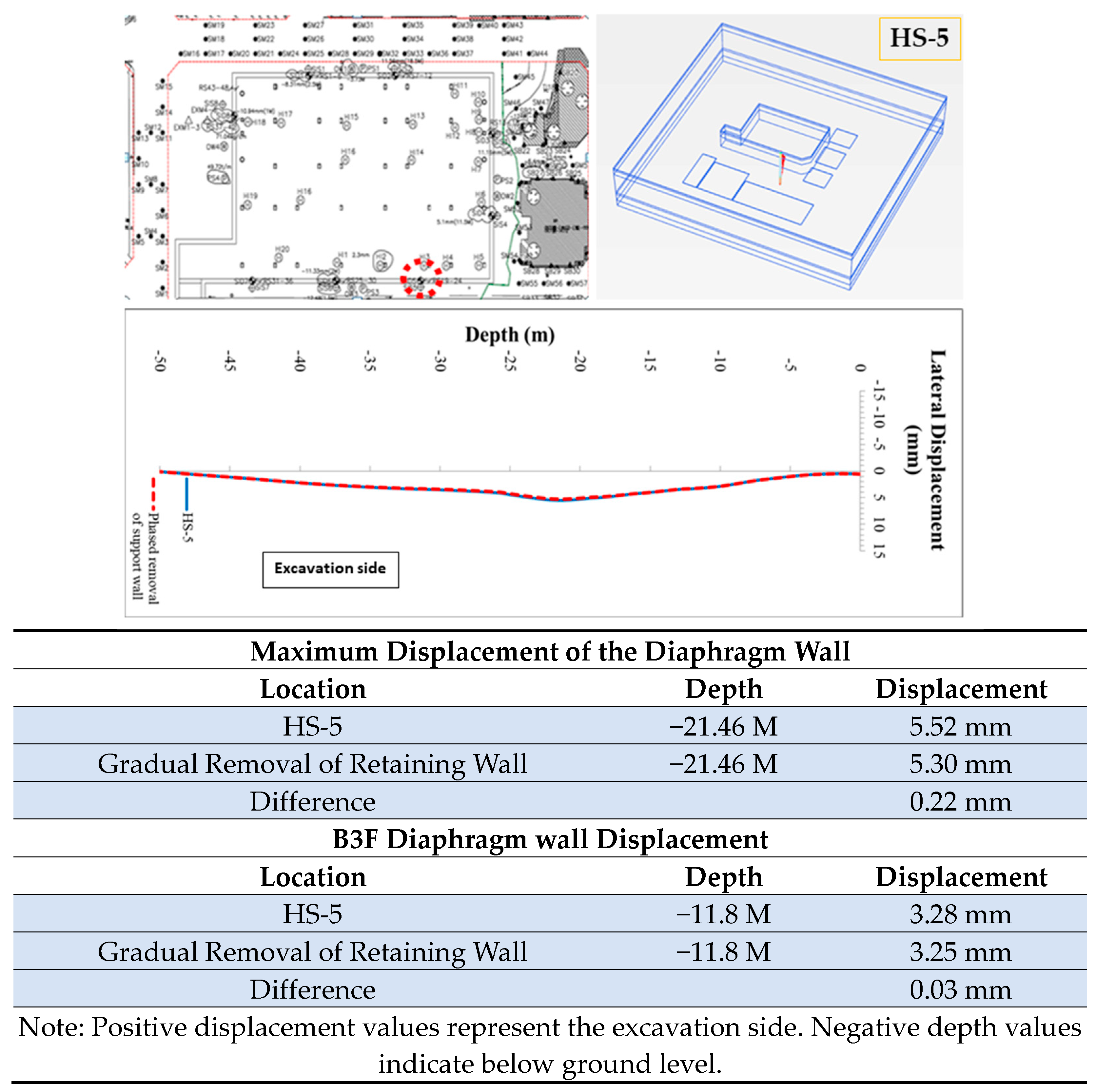
- On the direct southern side, analysis from HS-5 (Figure A1) indicates:
- Maximum lateral displacement with immediate strut removal was 5.52 mm.
- Delaying B3F strut removal until after B5F completion resulted in a maximum lateral displacement of 5.30 mm.
- This leads to a difference of 0.22 mm and a DRR of 3.98%. One reason might be the proximity to the margin and the reinforcing effect of the vertical diaphragm wall.
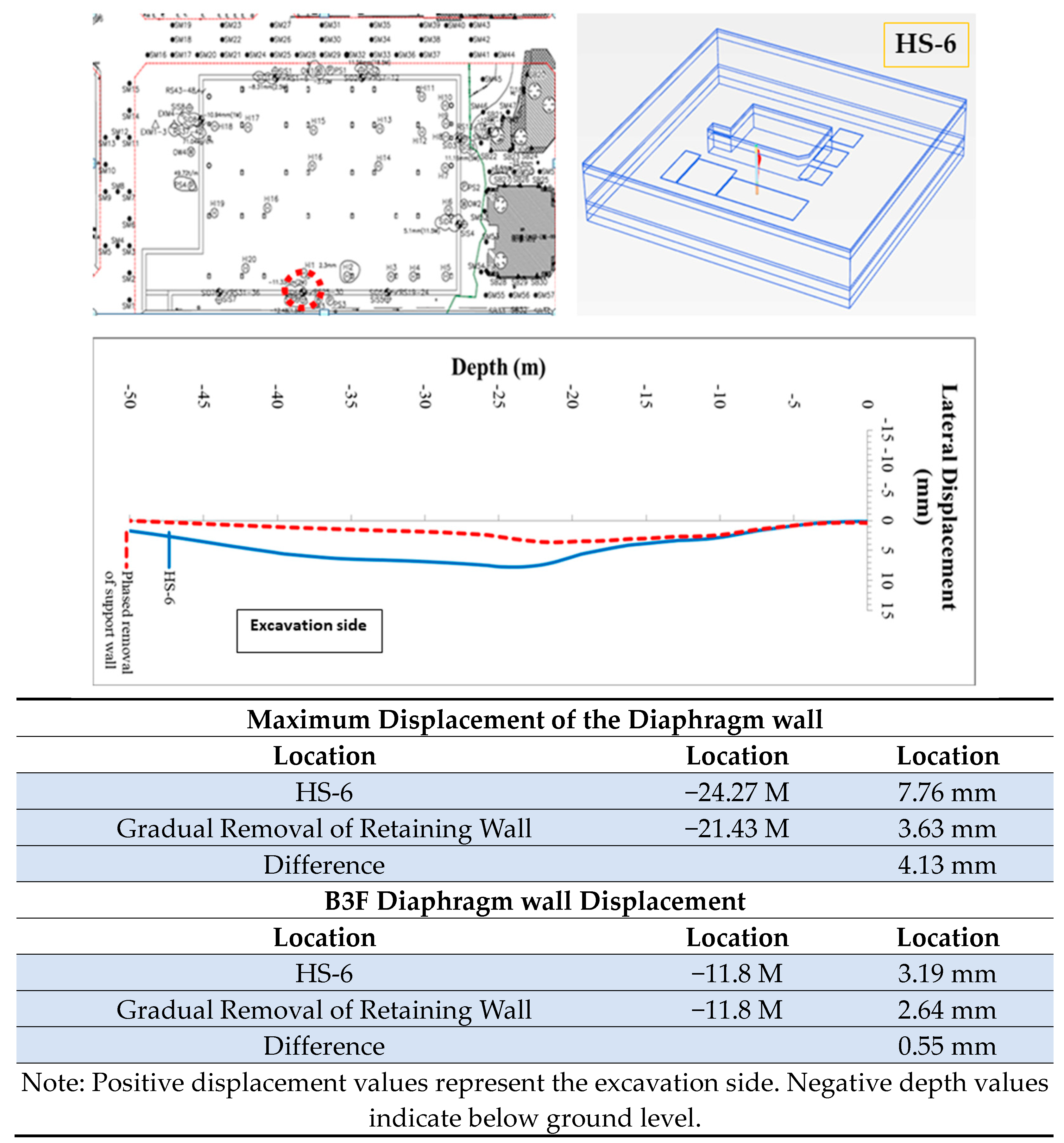
- For the southeast side, as deduced from HS-6 (Figure A2):
- Maximum lateral displacement with immediate strut removal was 7.76 mm.
- With the delayed removal approach, it reduced to 3.63 mm.
- The displacement difference amounted to 4.13 mm, with a DRR of 53.22%. This could be due to its central location on the diaphragm wall.
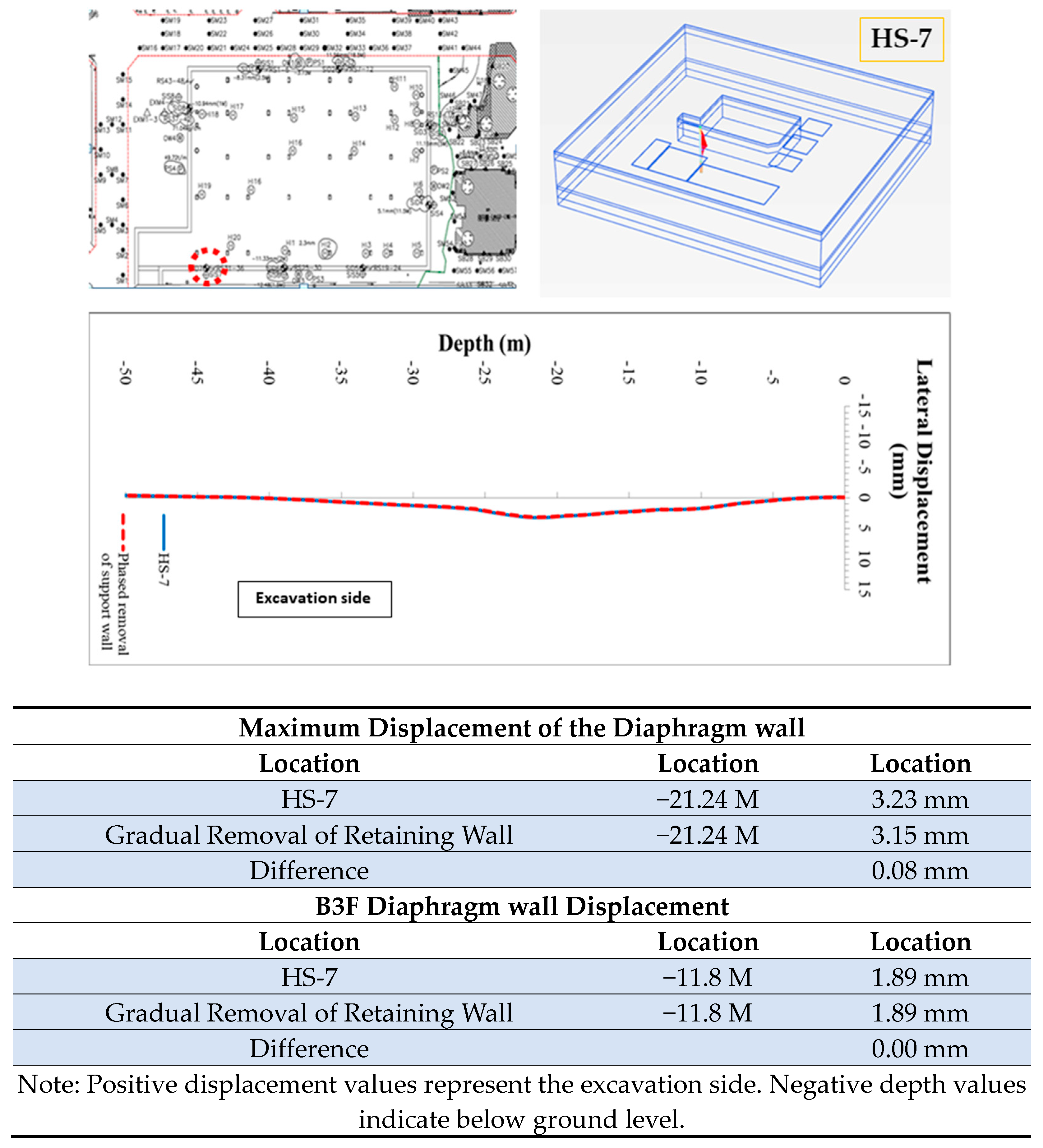
- On the southwest side, data from HS-7 (Figure A3) reveals:
- The maximum lateral displacement with immediate strut removal was 3.23 mm.
- The delayed approach yielded a displacement of 3.15 mm.
- This equates to a 0.08 mm difference and a DRR of 2.47%. This might be attributed to its proximity to the edge, leading to reduced deformation due to the reinforcing effect of the vertical diaphragm wall.
5. Conclusions
5.1. Conclusions
- Conclusions derived from numerical analysis simulation and validation include:
- The site in question is rectangular in shape. Simulation results on the shorter east-west sides closely match observed data. On the northern longer side, due to evenly spaced retaining and diaphragm walls, the simulated results also align closely with observations. However, for the southern longer side, which features irregularly placed retaining and diaphragm walls with multiple corner transitions, there is a notable difference between the simulation and observed data.
- According to the research by Ou [19], the mechanism by which retaining walls control wall displacement primarily stems from the friction between the retaining wall and the soil, as well as the bearing capacity at the end of the retaining wall. This leads to a complex mechanical behavior, making simulations more challenging and less accurate.
- Additionally, top-down construction methods tend to offer better control over wall displacement. However, monitoring often entails human errors, resulting in imprecisions between simulations and observed values. As a result, trends rather than actual measurements in displacement are often relied upon for verification.
- The study indicates that the trend in lateral displacement is consistent with numerical analysis results. For surface subsidence, the observed values exceeded simulation predictions due to repeated resurfacing of the adjacent AC road. When factoring in the effects of repeated road resurfacing and observational errors, the analytical results can be considered consistent with the actual situation.
- Conclusions regarding the timing of retaining wall removal include:
- On the direct southern side, analysis from HS-6 shows a Displacement Reduction Rate (DRR) of 53.22%. This can be attributed to its position between the Diaphragm Wall, which inherently exhibits larger displacements and thus has more pronounced reduction effects.
- On the southeast side, HS-5 analysis indicates a DRR of 3.98%. Being closer to the edge, and influenced by the reinforcing effects of the vertical Diaphragm Wall, the inherent displacements are smaller, leading to less significant reduction effects.
- On the southwest side, analysis from HS-7 reveals a DRR of 2.47%. Similar to the southeast side, being closer to the edge and under the influence of the vertical Diaphragm Wall, the inherent displacements are minimal, resulting in less pronounced reduction effects.
5.2. Recommendations
- Simulations indicate that adjusting the removal timing of retaining walls based on functional needs and linking them to floor slabs to form a T-shaped structure can effectively control wall displacement. For deeper basement levels, where temporary support is not available, this method can be considered to minimize displacement.
- This study solely analyzed the staggered removal of the B3F southern retaining wall. Future studies could consider not removing all retaining walls and analyzing the relationship with wall thickness. If the results are significant, adjustments to the retaining wall’s thickness could be made, potentially reducing construction costs or incorporating it as a permanent structural component.
- Typically, in top-down projects during the final excavation phase, due to a longer unsupported length from deeper excavations, horizontal or diagonal bracing is required to control lateral wall displacement. However, this procedure is time-consuming and poses higher operational risks, increasing construction hazards. Future studies might explore the effects of not removing retaining and diaphragm walls during the final excavation phase on wall displacement control.
Supplementary Materials
Author Contributions
Funding
Data Availability Statement
Conflicts of Interest
Appendix A


References
- Jian, Z.; Olivia, K. An introduction to connectivity concept and an example of physical connectivity evaluation for underground space. Tunn. Undergr. Space Technol. 2016, 55, 205–213. [Google Scholar] [CrossRef]
- Hsieh, P.-G.; Ou, C.-Y.; Lin, Y.-K.; Lu, F.-C. Lessons learned in design of an excavation with the installation of buttress walls. J. GeoEng. 2015, 10, 63–73. [Google Scholar]
- Shi, J.; Liu, G.; Huang, P.; Ng, C.W.W. Interaction between a large-scale triangular excavation and adjacent structures in Shanghai soft clay. Tunn. Undergr. Space Technol. 2015, 50, 282–295. [Google Scholar] [CrossRef]
- Hong, Y.; Ng, C.W.W.; Liu, G.B.; Liu, T. Three-dimensional deformation behaviour of a multi-propped excavation at a “greenfield” site at Shanghai soft clay. Tunn. Undergr. Space Technol. 2015, 45, 249–259. [Google Scholar] [CrossRef]
- Chen, R.; Meng, F.; Li, Z.; Ye, Y.; Ye, J. Investigation of response of metro tunnels due to adjacent large excavation and protective measures in soft soils. Tunn. Undergr. Space Technol. 2016, 58, 224–235. [Google Scholar] [CrossRef]
- Whittle, A.; Davies, R. Nicoll Highway collapse: Evaluation of geotechnical factors affecting design of excavation support system. In Proceedings of the International Conference on Deep Excavations, Singapore, 28–30 June 2006; p. 30. [Google Scholar]
- Abdi, A.S.; Ou, C.-Y. Numerical Study of the Effect of Ground Improvement on Basal Heave Stability for Deep Excavations in Normally Consolidated Clays. J. Geotech. Geoenviron. Eng. 2023, 149, 04023042. [Google Scholar] [CrossRef]
- Mana, A.I.; Clough, G.W. Prediction of movements for braced cuts in clay. J. Geotech. Eng. Div. 1981, 107, 759–777. [Google Scholar] [CrossRef]
- Ou, C.-Y.; Hsieh, P.-G.; Chiou, D.-C. Characteristics of ground surface settlement during excavation. Can. Geotech. J. 1993, 30, 758–767. [Google Scholar] [CrossRef]
- Clough, G.W.; O’Rourke, T.D. Construction-Induced Movements of In Situ Wall, Design and Performance of Earth Retaining Structure; ASCE: Reston, VA, USA, 1990; pp. 439–470. [Google Scholar]
- Masuda, T.; Einstein, H.H.; Mitachi, T. Prediction of lateral deflection of diaphragm wall in deep excavations. Doboku Gakkai Ronbunshu 1994, 1994, 19–29. [Google Scholar] [CrossRef] [PubMed]
- Wu, P.-Z.; Wang, M.-J.; Peng, Y.-R. Investigation of Continuous Wall Deformation Behavior. In Proceedings of the 7th Geotechnical Engineering Research Symposium, Taiwan, 7–11 September 1997; pp. 601–608. [Google Scholar]
- Wang, J.-Z.; Chan, X.-S.; Lei, Y.-M. Analysis of Soil Parameters in the Kaohsiung Metro Red Line Section. J. Chin. Inst. Civ. Hydraul. Eng. 2003, 30, 101–104. [Google Scholar]
- Surarak, C. Geotechnical Aspects of the Bangkok MRT Blue Line Project; Griffith University: Nathan, Australia, 2011. [Google Scholar]
- Peck, B. Deep excavation and tunnelling in soft ground, State of the art volume. In Proceedings of the 7th ICSMFE, Mexico City, Mexico, 29 August 1969; pp. 225–290. [Google Scholar]
- Ou, C.-Y.; Chiou, D.-C.; Wu, T.-S. Three-dimensional finite element analysis of deep excavations. J. Geotech. Eng. 1996, 122, 337–345. [Google Scholar] [CrossRef]
- Ou, C.; Liao, J.; Lin, H. Performance of a topdown basement construction. J. Geotech. Geoenviron. Eng. 1998, 9, 798–808. [Google Scholar] [CrossRef]
- Avanti, A. Numerical Analyses of Jakarta MRT Deep Excavation Project; National Taiwan University of Science and Technology: Taipei, Taiwan, 2013. [Google Scholar]
- Ou, C.-Y. Finite element analysis of deep excavation problems. J. Geoengin. 2016, 11, 1–12. [Google Scholar]
- Liao, R.-T. Performances of a Top Down Deep Excavation; National Taiwan University of Science and Technology: Taipei, Taiwan, 1996. [Google Scholar]
- Wang, J.-Z. Undrained Creep Behavior of Soft Clay Induced by Deep Excavation; National Taiwan University of Science and Technology: Taipei, Taiwan, 1997. [Google Scholar]
- Hsieh, P.-G. Prediction of Ground Movements Caused by Deep Excavation in Clay; National Taiwan University of Science and Technology: Taipei, Taiwan, 1999. [Google Scholar]
- Hsieh, P.-G.; Lin, Y.-L.; Ou, C.-Y. Three-Dimensional Numerical Analysis and Performance of Deep Excavation with Cross Walls and Buttress Walls. J. Chin. Inst. Civ. Hydraul. Eng. 2010, 22, 11–22. [Google Scholar] [CrossRef]
- Chen, S.-L.; Ho, C.-T.; Li, C.-D.; Gui, M.-W. Efficiency of buttress walls in deep excavations. J. GeoEng. 2011, 6, 145–156. [Google Scholar]
- Khoiri, M.; Ou, C.-Y. Evaluation of deformation parameter for deep excavation in sand through case histories. Comput. Geotech. 2013, 47, 57–67. [Google Scholar] [CrossRef]
- Ou, C.-Y.; Hsieh, P.-G.; Lin, Y.-L. A parametric study of wall deflections in deep excavations with the installation of cross walls. Comput. Geotech. 2013, 50, 55–65. [Google Scholar] [CrossRef]
- Ye, C.-Y. Efficiency of Buttress Walls and Cross Walls in Deep Excavation; National Taipei University of Technology: Taipei, Taiwan, 2012. [Google Scholar]
- Fong, J.-W. Numerical Analysis of Buttress Walls and Cross Walls in Deep Excavation; National Taipei University of Technology: Taipei, Taiwan, 2015. [Google Scholar]
- Hsieh, P.-G.; Ou, C.-Y. Shape of ground surface settlement profiles caused by excavation. Can. Geotech. J. 1998, 35, 1004–1017. [Google Scholar] [CrossRef]
- Ladd, R.S. Specimen Preparation and Cyclic Stability of Sands. J. Geotech. Eng. Div. 1977, 103, 535–547. [Google Scholar] [CrossRef]
- Ou, C.-Y. Deep Excavation Engineering: Analysis, Design Theories and Practices; Science and Technology Books: Taipei, Taiwan, 2002. [Google Scholar]
- Ou, C.Y. Advanced Deep Excavation Engineering Analysis and Design; Tech Books Incorporated: Taipei, Taiwan, 2017. [Google Scholar]
- Civil Engineering Association of Taipei City. Practical Manual for Excavation and Earth Retaining Support Engineering Design; Civil Engineering Association of Taipei City: Taipei, Taiwan, 2002. [Google Scholar]


| Layer | Soil Layer Description | Layer Bottom Distribution Depth (GL.−m) | Average Distribution Elevation (GL.−m) |
|---|---|---|---|
| 1 | Backfill Layer (SF) | 0.1~0.9 (0.5) | 0.0~0.5 |
| 2 | Silty Clay Layer (CL) | 1.8~3.7 (3.0) | 0.5~3.0 |
| 3 | Silty Sand Layer (SM) | 9.2~10.6 (9.9) | 3.0~9.9 |
| 4 | Silty Clay Layer (CL) | 19.8~27.4 (23.1) | 9.9~23.1 |
| 40.0~41.5 (40.7) | 23.1~40.7 | ||
| 5 | Silty Sand Layer (SM) | 40.9~45.0 (42.2) | 40.7~42.2 |
| 6 | Silty Clay Layer (CL) | 51.9~54.3 (52.7) | 42.2~54.7 |
| 7 | Gravel Layer (GW/GP) | - (Drilling Depth) | >52.7 |
| Modulus | Clay | Sand |
|---|---|---|
| Soil Unloading Elastic Modulus | ||
| Soil Shear Elastic Modulus | ||
| Soil Bulk Elastic Modulus |
| Soil Type | Poisson’s Ratio ν |
|---|---|
| Saturated Clay (Undrained) Unsaturated Clay (Undrained) Silty Sandy Clay | 0.5 0.35–0.4 0.3–0.4 |
| Silty Sand Sand and Gravel Soil Silt Soil Rock Concrete | 0.3–0.4 0.15–0.35 0.3–0.35 0.1–0.4 (varies by type) 0.15 |
| Item No. | Soil Layer | Depth (m) | γunsat (kN/m3) | γsat (kN/m3) | c’ (kN/m2) | φ’ (°) | E50ref (kN/m2) | Eoedref (kN/m2) | Eurref (kN/m2) | νur | ψ | m |
|---|---|---|---|---|---|---|---|---|---|---|---|---|
| #1 | SF | −0.5 | 19.1 | 19.6 | 0.5 | 30 | 20,000 | 20,000 | 60,000 | 0.20 | 0 | 0.5 |
| #2 | CL1 | −3.0 | 19.0 | 19.3 | 0.7 | 29 | 9000 | 7200 | 27,000 | 0.20 | 0 | 1.0 |
| #3 | SM1 | −10.0 | 19.5 | 20.1 | 0.7 | 30 | 28,000 | 28,000 | 84,000 | 0.20 | 0 | 0.5 |
| #4 | CL2 | −40.0 | 18.8 | 19.0 | 1.1 | 30 | 17,000 | 13,600 | 51,000 | 0.20 | 0 | 1.0 |
| #5 | SM2 | −43.0 | 19.0 | 19.5 | 1.0 | 31 | 34,500 | 34,500 | 103,500 | 0.20 | 1.0 | 0.5 |
| #6 | CL3 | −53.0 | 19.2 | 19.5 | 1.5 | 31 | 19,000 | 15,200 | 57,000 | 0.20 | 1.0 | 1.0 |
| #7 | GW | −62.0 | 21.5 | 21.7 | 1.0 | 35 | 70,000 | 70,000 | 210,000 | 0.20 | 5.0 | 0.5 |
| Soil Parameter | Soil Parameter Selection Description | |||||||||||
| Drainage Properties | According to the PLAXIS manual, a model’s drainage behavior can be categorized into drained, undrained A, undrained B, undrained C, and impervious scenarios. Given that sandy soil quickly expels excess pore water pressure due to its larger voids, effective stress analysis with drainage behavior is utilized. Clay sections are modeled with undrained behavior, and for analysis consistency with sandy soil, the undrained A scenario is chosen. Undrained A uses effective stiffness and strength parameters to simulate undrained behavior. | |||||||||||
| Wet Soil Unit Weight γt, Effective Cohesion c′, Effective Friction Angle 𝜙′ | Values for wet soil unit weight, effective cohesion, and effective friction angle can be derived from drilling reports and laboratory tests. The PLAXIS manual suggests inputting a slightly larger value when effective cohesion is 0 to speed up analysis. | |||||||||||
| Void Ratio e, Specific Gravity Gs | The soil parameter table in this study did not provide specific gravity and void ratio data. Following recommendations from Ou’s “Deep Excavation Engineering Analysis, Design Theory, and Practice”, an assumption was made that each soil layer has a specific gravity of 2.7 [31]. The void ratio was then inferred using the saturated unit weight and specific gravity. | |||||||||||
| Soil Elastic Modulus Es | Attention is crucial when analyzing sandy soil in deep excavation projects. Based on research by Ou et al. [26], the effective internal friction angle reflects the friction between soil particles, related to the roughness, shape, and compression of the soil particles. The elastic modulus is associated with the physical properties and inter-particle forces. In practice, empirical formulas often estimate these. In this research, the soil layers utilized the Hardening Soil Model, with the soil parameters summarized in Table 5. According to Khoiri and Ou [25], the recommended elastic modulus Es for sandy soil using the HS model ranges from Es = 2000–4000 N. This study adopts Es = 3000 N. | |||||||||||
| Permeability Coefficient K | Based on Ou [31], various soil types’ permeability coefficients have been collated. This study adopted the permeability coefficients for Taipei silty clay K = (0.5 − 2.0) × 10−7 cm/s and Taipei silty sand K = (0.5 − 6.0) × 10−4 cm/s. | |||||||||||
| Poisson’s Ratio ν | Ou [31] provided ranges for the Poisson’s ratio of various soils, as shown in Table 6. | |||||||||||
| Other Relevant Parameters | The parameters obtained from empirical formulas, drilling reports, and laboratory experiments are listed in Table 7. | |||||||||||
| Item | Material Type | Thickness t (m) | Distribution Depth d (m) | (kN/m3) | Modulus of Elasticity E (kN/m2) | Poisson’s Ratio ν’ |
|---|---|---|---|---|---|---|
| 2F Neighbor | Plate | 1.0 | 0 | 20.0 | 2.1 | 0.15 |
| 3F Neighbor | Plate | 1.3 | 0 | 30.0 | 2.1 | 0.15 |
| 6F Neighbor | Plate | 2.1 | 0 | 50.0 | 2.1 | 0.15 |
| 11F Neighbor | Plate | 3.1 | 0 | 90.0 | 2.1 | 0.15 |
| 14F Neighbor | Plate | 3.8 | 0 | 100.0 | 2.1 | 0.15 |
| Road | 5.0 | 9.81 | 0.15 |
| Item | Thickness (m) | Unit Weight γ (kN/m3) | Young’s Modulus E (kN/m2) | Poisson’s ratio υ | fc’ (kg/cm2) | Remark (Ou [32]) |
|---|---|---|---|---|---|---|
| Diaphragm wall (DW) | 1.2 | 24 | 1.48 × 10⁷ | 0.17 | 280 | Reduction coefficient of 0.6 |
| Buttress walls, Cross walls (BW&CW) | 0.6 | 24 | 1.48 × 10⁷ | 0.17 | 280 | Reduction coefficient of 0.6 |
| Floors 1F to B6F Slabs | 0.45 | 24 | 1.93 × 10⁷ | 0.17 | 350 | Reduction coefficient of 0.7 |
| Foundation Slab (FS) | 1.2 | 24 | 1.93 × 10⁷ | 0.17 | 350 | Reduction coefficient of 0.7 |
| Inclinometer ID | HS Model (Plaxis 3D 2018) | Actual Monitoring Data | Remark | ||
|---|---|---|---|---|---|
| Depth (Location) | Displacement Value | Depth (Location) | Displacement Value | ||
| SID-1 | −21.35 M | −5.06 mm | −22.00 M | −5.33 mm | North side |
| SID-2 | −21.42 M | −5.68 mm | −23.00 M | −8.18 mm | North side |
| SID-3 | −21.80 M | −7.06 mm | −18.00 M | −6.74 mm | East side |
| SID-4 | −20.90 M | −3.51 mm | −21.00 M | −3.6 mm | East side |
| SID-5 | −21.46 M | −5.52 mm | −25.00 M | −5.86 mm | South side |
| SID-6 | −24.27 M | −7.76 mm | −25.00 M | −10.32 mm | South side |
| SID-7 | −21.24 M | −3.23 mm | −21.00 M | −4.30 mm | South side |
| SID-8 | −21.46 M | −6.73 mm | −25.00 M | −6.79 mm | West side |
| Point | Source | Phase 1 Excavation | Phase 2 Excavation | Phase 3 Excavation | Phase 4 Excavation | Phase 5 Excavation | Phase 6 Excavation | Phase 7 Excavation | Phase 8 Excavation |
|---|---|---|---|---|---|---|---|---|---|
| SM21~SM23 | Analyzed Values | −13.52 | −13.54 | −13.42 | −13.05 | −13.13 | −13.37 | −13.91 | −14.69 |
| (North) | Measured Values | −8.8 | −8.8 | −12.6 | −13.00 | −13.00 | −13.50 | −13.90 | −19.00 |
| SM29~SM31 | Analyzed Values | −13.76 | −13.88 | −13.90 | −13.58 | −13.65 | −13.88 | −14.49 | −15.33 |
| (North) | Measured Values | −8.0 | −8.50 | −9.90 | −10.90 | −11.30 | −12.60 | −13.60 | −18.50 |
| SM37~SM39 | Analyzed Values | −13.11 | −13.18 | −13.14 | −12.84 | −12.92 | −13.16 | −13.72 | −14.53 |
| (North) | Measured Values | −8.7 | −9.50 | −10.80 | −12.60 | −12.00 | −13.50 | −14.30 | −18.10 |
| SM11~SM13 | Analyzed Values | −12.16 | −12.27 | −12.43 | −12.5 | −12.66 | −12.87 | −13.27 | −13.74 |
| (West) | Measured Values | −5.10 | −6.40 | −7.50 | −8.10 | −9.20 | −9.80 | −11.10 | −15.10 |
| SM3~SM5 | Analyzed Values | −13.17 | −13.10 | −12.97 | −12.76 | −12.89 | −13.15 | −13.58 | −14.21 |
| (West) | Measured Values | −7.30 | −9.20 | −10.90 | −12.40 | −13.30 | −13.60 | −14.60 | −15.90 |
Disclaimer/Publisher’s Note: The statements, opinions and data contained in all publications are solely those of the individual author(s) and contributor(s) and not of MDPI and/or the editor(s). MDPI and/or the editor(s) disclaim responsibility for any injury to people or property resulting from any ideas, methods, instructions or products referred to in the content. |
© 2023 by the authors. Licensee MDPI, Basel, Switzerland. This article is an open access article distributed under the terms and conditions of the Creative Commons Attribution (CC BY) license (https://creativecommons.org/licenses/by/4.0/).
Share and Cite
Hsu, C.-F.; Kuan, C.-F.; Chen, S.-L. Three-Dimensional Numerical Analysis on the Influence of Buttress Wall Removal Timing on the Lateral Deformation of Diaphragm Walls during Deep Excavation. Buildings 2023, 13, 2678. https://doi.org/10.3390/buildings13112678
Hsu C-F, Kuan C-F, Chen S-L. Three-Dimensional Numerical Analysis on the Influence of Buttress Wall Removal Timing on the Lateral Deformation of Diaphragm Walls during Deep Excavation. Buildings. 2023; 13(11):2678. https://doi.org/10.3390/buildings13112678
Chicago/Turabian StyleHsu, Chia-Feng, Chung-Fu Kuan, and Shong-Loong Chen. 2023. "Three-Dimensional Numerical Analysis on the Influence of Buttress Wall Removal Timing on the Lateral Deformation of Diaphragm Walls during Deep Excavation" Buildings 13, no. 11: 2678. https://doi.org/10.3390/buildings13112678