Modeling Performance and Uncertainty of Construction Planning under Deep Uncertainty: A Prediction Interval Approach

Abstract

In construction planning, decision making has a great impact on final project performance. Hence, it is essential for project managers to assess the construction planning and make informed decisions. However, disproportionately large uncertainties occur during the construction planning stage; in the worst case, reliable probability distributions of uncertainties are sometimes unavailable due to a lack of information before construction implementation. This situation constitutes a deep uncertainty problem, making it a challenge to perform a probability-based uncertainty assessment. The current study proposes a modeling approach that applies prediction intervals for construction planning via the integration of discrete-event simulation (DES), fuzzy C-means clustering (FCM), Bayesian regularization backpropagation neural networks (BRBNNs), and particle swarm optimization (PSO). The DES is used to perform data sampling of the construction alternatives and assess their performances under uncertainty. Based on the generated samples, the FCM, BRBNN, and PSO are integrated in a machine learning algorithm to model the prediction intervals that represent relationships between construction planning schemes, performances, and the corresponding uncertainties. The proposed approach was applied to a case project, with the results indicating that it is capable of modeling construction performance and deep uncertainties with a defined 95% confidence level and fluctuation within 1~9%. The presented research contributes a new and innovative option, using prediction intervals to solve deep uncertainty problems, without relying on the probability of the uncertainty. This study demonstrates the effectiveness of the proposed approach in construction planning.

1. Introduction

Construction planning is the stage before actual construction during which preliminary decisions related to construction resources, schedules, and other schemes are made. Over the past few decades, many studies such as various research conducted by the Construction Industry Institute (CII) have revealed how construction planning can significantly influence final project performance [1]. Therefore, decision making during the construction planning stage needs to be carefully considered to obtain the expected construction outcomes.

The assessment of construction performance at the planning stage enables managers to compare different construction schemes in order to make an informed decision. Thus, an appropriate tool for the assessments related to the construction planning phase is needed. However, uncertainty has long been considered an obstacle of accurate assessments of construction performances during the construction planning stage [2]. Uncertainties about labor work productivity, equipment failure rates, weather, or off-site transport conditions are a few examples of factors that can challenge reliable predictions of construction progress. Previous studies have suggested that construction uncertainty can cause 30–35%, 25–40%, and 26% fluctuations in construction duration [3], project cost [4], and environment impacts [5], respectively. Indeed, uncertainty challenges the entire construction process, but a disproportionately large part occurs during the construction planning stage because the information relevant to a project has not been fully determined before construction implementation [2]. Moreover, many previous studies have found that estimations of uncertainty performed at the planning stage may largely differ from the actual situation [6].

The existence of uncertainty makes it challenging to assess construction performance accurately during the construction planning stage. Ibadov and Kulejewski [7] thus stated that the uncertainty analysis approaches for construction planning are critical to the success of construction projects. To address this, uncertainty in the assessments of the construction planning stage has previously been treated as random variables, which are normally described by probability distributions [8], and probability-based methods, such as the Monte Carlo method, have been widely used [9]. Probability-based methods will predefine the probability distribution of uncertain factors, an action which often requires sufficient historical experience or statistical data.

However, these methods may not always be applicable to the construction planning stage. For example, Sadeghi et al. [10] proposed that it is sometimes not feasible to collect the required information to develop reliable probability distributions for all of the uncertainties related to a construction project. In addition, the uniqueness of certain construction projects, such as mega buildings or infrastructure, may make it impossible to find sufficient historical data to develop reliable probability distributions due to the limited similarities to any previous projects [11]. In these situations, the uncertainty originates from a lack of knowledge. According to both Walker et al. [12] and Bryant and Lempert [13], a situation challenged by uncertain probability distributions is a deep uncertainty problem. Many previous studies [14,15] found that probability-based methods have difficulties in handling deep uncertainty problems. Thus, these types of problems require a new method that can complement the current probability-based methods for managing uncertainty.

This study proposes a prediction interval approach for modeling construction performance under deep uncertainty which integrates discrete-event simulation (DES), fuzzy C-means clustering, Bayesian regularization backpropagation neural networks (FCM-BRBNN), and particle swarm optimization (PSO). First, the DES is applied to simulate the performance of various construction alternatives under deep uncertainty conditions and generate a dataset that contains the construction schemes, uncertainties, and corresponding project performances. A machine learning algorithm constructed based on fuzzy C-means clustering and Bayesian regularization backpropagation neural networks is then applied to the dataset with the objective of directly extracting the relationship between construction schemes and uncertainties of the final performance. The PSO, as an intelligent optimization method, is used to identify the optimal hyper-parameters of the machine learning model to ensure optimal modeling.

Thus, instead of relying on precise probability distributions, the proposed approach uses a large and relevant dataset to directly capture the underlying effects of construction planning in light of deep uncertainty, which is a complement to the shortcomings of heavily relying on probability distributions of the existing methods. Specifically, the assessment of the construction performance is represented through prediction intervals, which specify the lower and upper limits within which future project performance is expected to fall under deep uncertainty for a pre-defined confidence level (e.g., 90 or 95%). The research is the first attempt to use prediction intervals to solve deep uncertainty problems.

2. Background

A construction project will involve many decisions. From all decisions, construction planning is the period between a contract being awarded and construction implementation; this phase involves important decision making such as choosing a construction strategy, determining the construction schedule, and arranging for the resources required for project execution. Additional decisions, such as updates to the project plan, will be made during construction implementation based on the information about progress and adjustments [16]. Previous studies have suggested that the decisions made during construction planning play a relatively significant role in the eventual success of a project [17]. The MacLeamy curve also illustrated this relationship (see Figure 1). The construction planning phase is associated with a relatively larger ability to influence project performance than later phases in the project life cycle. As such, the level of influence on a project declines as the construction implementation begins, and the cost of making changes increases after that.

However, the degree of uncertainty about the future state of the project is high at early stages (see Figure 1); for this reason, project performance, e.g., project duration and cost, is affected by a large degree of fluctuation, which arises from uncertainty [20]. Thus, the uncertainty in early planning stages presents a challenge for assessing construction performance and making informed decisions. In construction projects, contractors must have the ability to evaluate how uncertainty will impact construction performance in order to make the correct decisions on plans.

Many studies that have focused on assessing how uncertainty influences construction performance treat uncertainty as a factor that is represented by random variables [8,21]; this is also termed aleatoric uncertainty. Most previous research has considered random variables such as weather, labor productivity, material wastage, and more. When approaching an uncertainty analysis, researchers often rely on predefined probability distributions of uncertain factors; this enables the application of probability-based methods such as Monte Carlo (MC) simulation and the Program Evaluation and Review Technique (PERT). These methods are used to estimate the possible future state of uncertainty so as to assess the possible construction outcomes [22,23]. However, a robust uncertainty analysis requires data from sufficient similar projects or historical experience to obtain reliable probability distributions [24]. In many situations this is either impossible or extremely costly if it is only in the construction planning stage [10], which makes the probability-based methods unapplicable.

In addition, recent research has found that construction projects are also exposed to epistemic uncertainty [25], which is uncertainty arising from a lack of information and knowledge [26]. The presence of epistemic uncertainty in construction can be explained by the uniqueness of each project, i.e., prior projects and contractors’ experience are not closely related to the characteristics of a novel and unique project [8]. In addition, no observations of the actual construction are available during the construction planning stage. As such, probability-based methods are not applicable to these types of situations [27]. As an example, Feng et al. [28] found that estimating the probability distributions for various sources of uncertainty could obscure the actual future state and, even worse, lead to inaccurate performance estimations and biased decisions.

Therefore, the limited information available during the construction planning stage means that the probability distribution of certain uncertain factors that influence project implementation will be likewise uncertain. Walker et al. [12] divided the uncertainty system into five levels according to the progressive degree of uncertainty. Within this taxonomy, situations in which the probability distributions of uncertain factors are uncertain represent a deep uncertainty problem. Previous studies have suggested that traditional, probability-based methods will face challenges when applied to deep uncertainty problems [12,14].

Machine learning algorithms could be a promising solution for the deep uncertainty problems described above. In previous studies, machine learning algorithms were successfully applied to deal with construction performance modeling due to the advantage in knowledge extraction and knowledge learning [29,30,31]. Furthermore, machine learning algorithms have successfully quantified uncertainties from appropriately large datasets without relying on probability distributions [32]. Hence, machine learning could be relevant and promising to modeling deep uncertainty in construction planning. On the other hand, construction simulation technologies can explore various construction scenarios and obtain construction performance data, which—theoretically—can serve as a resource for machine learning in extracting the construction performances of a project associated with deep uncertainty. The present research was conducted to investigate the possibility of integrating construction simulation technology and machine learning to model construction performances affected by deep uncertainty.

3. Prediction Intervals Modeling Approach

The flowchart of the prediction interval modeling approach for construction planning is illustrated in Figure 2. As shown in Figure 2, the proposed approach consists of two main modules—(1) construction sample generation and (2) performance uncertainty modeling—and an auxiliary module, modeling optimization. Following the flowchart, the possible construction performance range under deep uncertainty can be obtained during the construction planning stage without relying on probability distributions.

In the proposed approach, the first module is construction sample generation, during which the full information samples (FIS), including construction schemes, the state of uncertain factors, and corresponding construction performances (e.g., duration and cost), are obtained by discrete-event simulation (DES). The FIS are then imported into the second module for uncertainty modeling.

The second module is performance uncertainty modeling, during which the fuzzy C-means clustering and Bayesian regularization backpropagation neural network (FCM-BRBNN) integrated method are proposed to compute the prediction intervals for construction performances. More specifically, the samples are first clustered by FCM according to the features of construction schemes, with the baseline construction performance (i.e., average performance) of each sample modeled by the BRBNN algorithm. Next, prediction intervals for the clusters and each individual sample are calculated based on the residual errors between the baseline model outputs and the observed data, as well as the grade of the memberships in the clusters. The final stage of this module applies another BRBNN algorithm to explore the relationship between construction schemes and the corresponding performance prediction intervals. The resulting prediction intervals for performances (project duration and cost) by the developed BRBNN model can be used to reliably estimate the construction performances of various alternatives by inputting new construction schemes, without relying on probability distributions.

To increase the reliability (i.e., accuracy) and effectiveness (i.e., decision support) of modeling, particle swarm optimization (PSO) is applied in the auxiliary module to identify the optimal hyper-parameters for modeling from all possible settings, including the number of clusters, the number of hidden layers, and the neurons in each neural network. The developed model is designed to be both reliable and effective in assessing the performance and uncertainty of construction planning under deep uncertainty.

The following section will explain the three modules of the proposed approach in detail.

3.1. Construction Sample Generation

Process simulation technology is a useful tool for evaluating and predicting construction performance [33]. Process simulation during the planning stage of construction is advantageous, as it enables project managers to explore various construction scenarios and obtain the performance of every potential construction scheme. In the proposed method, DES was used for construction simulation to generate big datasets of full information samples (FIS) for subsequent uncertainty modeling due to its advantages in efficiently capturing how uncertainty influences construction schemes, as well as the interactions between construction processes [34].

In this study, the procedure for the DES-based construction process simulation is adapted from Tolk and Turnitsa [35] and Mohamed and AbouRizk [36], and it is presented in more detail in Figure 3. The basis for the simulation model is constructing a relationship between the real world, the concept world, and the simulation world. In this study, the real world is the real construction process, the conceptual world is the applied set of construction processes, and the simulation world is the computer model created from the conceptual model. The first step of the simulation model is conducting a detailed analysis of which construction processes will occur in the real world and collecting information related to the construction project, after which the purpose and scope of the construction process simulation will be identified. Following this step, an ontology-driven method [37] is used to map the construction processes, while the Component, Action, Resource, and Sequencing model (CARS) proposed by Fischer et al. [38] is adopted to detail the logics of construction for the conceptual model. The DES simulation model of construction processes can then be created on a computer platform based on the conceptual model, and the model is considered validated if the simulation results statistically agree with the actual construction project.

When developing the DES model, the construction parameters and uncertain factors are input into the simulation model to obtain the corresponding construction performances (e.g., project cost and duration, among others). In this study, for the deep uncertain factors which do not have reliable probability distributions, the possible value range, rather than the precise probability distribution, will be input into the DES model. The possible value range depends on the prior information related to the uncertainty and the decision maker’s judgement on the degree of uncertainty. Specifically, when decision makers deal with a problem having a high degree of deep uncertainty and are not confident in their estimates of uncertainty based on historical experience, the value range can be expanded appropriately; otherwise, it can be relatively small. Thus, compared with the probability-based methods, the introduction of a value range does not require more data to fit the probability distribution, which is more applicable to construction planning, and it does not require the assumption of the probability distribution and can thus avoid inaccurate performance estimations and biased decisions due to the incorrect assumption of probability distributions [15].

The construction performance simulated by the DES model, along with the construction schemes, constitute the full information samples (FIS) that will be transferred to the performance uncertainty modeling module and divided into three datasets in line with standard statistical learning protocols [39], namely, training, validation, and testing sets. The size of the full information samples (FIS) is determined by the accuracy of the modeling of the next module, which will be explained in detail in Section 4.3.

3.2. Performance Uncertainty Modeling

In the module of performance uncertainty modeling, the relationships between construction schemes and their performance will be extracted from the large FIS datasets. The extracted knowledge will then be used to model the construction performance and corresponding uncertainty in the deep uncertainty situation. As a result of deep uncertainty, theoretically, the assessment of construction performance will not provide a precise value. Therefore, the outcome of the second module is represented by prediction intervals (PIs), which describe uncertainty by specifying the lower and upper limits within which construction performance is expected to fall for a pre-set confidence level. A more detailed description of the statistics underlying PIs is provided by Shrestha and Solomatine [32] and Heskes [40].

A method that integrates fuzzy C-means clustering (FCM) and Bayesian regularization backpropagation neural networks (BRBNNs) is used in this study to obtain the PIs of construction performance. First, the BRBNN is applied to determine the relationship between the construction schemes and performance in the baseline prediction model. Then, FCM is used to cluster the sample according to the construction scheme and uncertainty features; the PIs of each cluster and sample are then calculated based on the residual errors between the baseline model and actual performance and the membership grade of the sample to the clusters. After obtaining the PIs for each sample, the BRBNN is used again to directly map the PIs to the construction scheme; this enables project managers to infer the construction performances at the planning stage without knowing precise probability distributions. The following sections will describe the presented methodology for supporting decision making under deep uncertainty in more detail.

3.2.1. Baseline Prediction Model

The baseline prediction model presented in this paper will use the full information samples (FIS) to infer how the tested construction schemes map to the baseline construction performance. In this model, baseline means that the mapping is inferred with average values and without considering the influence of uncertainty. To extract the relationship between construction schemes and their performances, various modeling techniques have been proposed, among which the artificial neural network is a powerful and ideal tool due to its accurate learning ability in the construction context [41]. BRBNN is a widely used artificial neural network with excellent generalization ability [42]. Foresee and Hagan [43] claimed that the introduction of Bayesian regularization in a backpropagation neural network further extends the generality of an artificial neural network. Based on the characteristics and advantages presented above, BRBNN was chosen as the learning algorithm in the model to determine the potential relationship between construction schemes and performances. The overall structure of the BRBNN in the baseline prediction model is represented in Figure 4.

As shown in Figure 4, the BRBNN consists of three layers or more: an input layer; a number of hidden layers; and an output layer. Each layer is composed of numbers of neurons which are connected by weighted links to transfer the information between layers [44]. In this study, the neurons in the input layer are the construction parameters which represent the various schemes, such as the different types and the number of construction resources, while the output neurons describe the construction performance (e.g., duration and cost). The number of hidden layers and their neurons determines the depth and complexity of the BRBNN model. Increasing the number of hidden layers and their neurons minimizes the difference between the observed data and the modeled output but reduces the generalization ability and may lead to an overfitting problem [41]. Thus, in this study, the optimal selection of the above two parameters is identified by the intelligent optimization method, which will be explained in detail in the Section 3.3.

After the BRBNN learning process, a target function describing the relationship between input and output variables will be obtained. Based on the function, the potential connections among construction schemes and corresponding baseline performances can be directly modeled. According to Bengio [45], the basis of BRBNN is represented as Equations (1) and (2).

$$a_i^{(j+1)}=g({\displaystyle \sum _{k=0}^{K_j}{\Theta }_{ik}^{(j)}{a}_k^{(j)}}),$$

(1)

$$g(z)=\frac{1}{1+e^{-z}},$$

(2)

where $a_i^{(j)}$ represents the activation of unit i in layer j, and $a_0^{(j)}$ = 1 represents the bias value. K_j is the number of units in layer j, ${\Theta }_{ik}^{(j)}$ is the weight mapping from unit k in layer j to unit i in layer j + 1, and g(·) is the activation function of neural networks.

The BRBNN improves the generalization ability of the learning model by introducing an additional regularization term into the cost function. The regularized cost function is represented as Equation (3) [46].

$$J(\Theta )=\alpha E_D+\lambda E_{\Theta },$$

(3)

where $J(\Theta )$ is the regularized cost function, $E_D$ is the squared sum of the residuals between the model outputs and observed data, $E_{\Theta }$ is the squared sum of the weights in the network (the weight of the bias value is excluded), and $\alpha$ and $\lambda$ are the regularization parameters.

In the BRBNN, the weights of the network are random variables, and their prior probability distribution is assumed to be Gaussian at the start of the analysis. When the output of the network is obtained, the posterior distribution of the weights will be updated according to Bayes’ rule [47] (see Equation (4)).

$$P(\Theta |D,\alpha ,\lambda ,H)=\frac{P(D|\Theta ,\lambda ,H)P(\Theta |\alpha ,H)}{P(D|\alpha ,\lambda ,H)},$$

(4)

where H is the network model, $\Theta$ is the network weight, D is the training set of the network model, $P(\Theta |\alpha ,H)$ is the prior distribution of the network weight without training set data, $P(\Theta |D,\alpha ,\lambda ,H)$ is the posterior distribution, $P(D|\Theta ,\lambda ,H)$ is the likelihood function, and $P(D|\alpha ,\lambda ,H)$ is the normalization factor.

After determining the weight value that maximizes posterior probability, the parameters $\alpha$ and $\lambda$ will be optimized according to Bayes’ rule [47] (see Equation (5)); more specifically, the values of $\alpha$ and $\lambda$ will maximize the posterior probability given the most probable network parameters. The network will continue to be trained using $\alpha$ and $\lambda$ until convergence is achieved.

$$P(\alpha ,\lambda |D,H)=\frac{P(D|\alpha ,\lambda ,H)P(\alpha ,\lambda |H)}{P(D|H)},$$

(5)

where $P(\alpha ,\lambda |H)$ and $P(\alpha ,\lambda |D,H)$ are the prior and posterior distributions of $\alpha$ and $\lambda$, respectively, $P(D|\alpha ,\lambda ,H)$ is the likelihood function, and $P(D|H)$ is the normalization factor.

3.2.2. Sample Clustering

In this study, the assessment of project performance is the prediction interval (PI) within which future performance is expected to fall. This interval is used to represent the expected project performance under deep uncertainty at the construction planning stage, before construction begins, and extensive project-related data are available. According to statistical theory, the samples with similar features have similar uncertainty characteristics [32]. Thus, the uncertainties of construction schemes in the same cluster will show a higher degree of similarity. Hence, the presented method will partition the construction schemes into a number of homogenous clusters that are based on construction parameters and identify the uncertainty performance of each sample through the uncertainty of the clusters. Clustering methods can be divided into hard clustering and fuzzy clustering depending on whether a sample belongs to strictly one cluster or not [48]. Previous studies have found that the boundaries between things in most cases are not distinct, which makes the fuzzy clustering method more flexible than the hard clustering method [48,49]. Fuzzy C-means (FCM) is one of the most popular fuzzy clustering methods; it has been widely applied to solve clustering problems in data mining [50]. In light of this, the fuzzy C-means (FCM) method is introduced to objectively establish the similarity among construction scheme samples and make fuzzy clusters.

The FCM method was initially proposed by Dunn [51] and then extended and generalized by Bezdek [52]. The purpose of the FCM method is to obtain a fuzzy partition which minimizes the cost function, as formulated in Equation (6). The procedure of finding the minimum is an iterative process, in which the parameters are constantly updated according to the constraints of Equations (7) and (8) until the termination condition is met, i.e., the cost function or the membership grade become stable.

$$J_m={\displaystyle \sum _{i=1}^N{\displaystyle \sum _{j=1}^C{u}_{ij}^m}}{\Vert x_i-c_j\Vert }^2,$$

(6)

$$c_j=\frac{{\displaystyle \sum _{i=1}^N{u}_{ij}^m{x}_i}}{{\displaystyle \sum _{i=1}^N{u}_{ij}^m}},$$

(7)

$$u_{ij}=\frac{1}{{\displaystyle \sum _{k=1}^C{(\Vert x_i-c_j\Vert /\Vert x_i-c_k\Vert )}^2}},$$

(8)

where $x_i$ is the ith construction scheme sample, $c_j$ is the center of the jth cluster, $u_{ij}$ is the membership grade of the ith sample in the jth cluster, $\Vert •\Vert$ is the Euclidean norm, and m is the weighting exponent, which is a constant in $\left[1,\infty \right]$.

3.2.3. Prediction Interval Calculation and Modeling

The prediction interval (PI) for each cluster is calculated based on the residual errors between the outputs from the baseline model and the corresponding observed data. To obtain a PI with the pre-set confidence level $\alpha \times 100\%$, the $(1-\alpha )/2\times 100$ and $(1+\alpha )/2\times 100$ percentile values of the residual errors are chosen for the lower and upper prediction intervals, respectively. Thus, all construction samples are first sorted in ascending order based on the residual error. The lower and upper prediction intervals for each cluster are then calculated using Equations (9) and (10), respectively [32].

$$PI{C}_k^l=e_i\hspace{1em}\mathrm{s}.\mathrm{t}. {\displaystyle \sum _{h=1}^i{u}_{hk}}<\frac{1-\alpha }{2}{\displaystyle \sum _{h=1}^n{u}_{hk}},$$

(9)

$$PI{C}_k^u=e_j\hspace{1em}\mathrm{s}.\mathrm{t}. {\displaystyle \sum _{h=1}^j{u}_{hk}}<(\frac{1+\alpha }{2}){\displaystyle \sum _{h=1}^n{u}_{hk}},$$

(10)

where $PI{C}_k^l$ and $PI{C}_k^u$ represent the lower and upper prediction intervals for the kth cluster, respectively, $u_{hk}$ is the membership grade of the hth sample in the kth cluster, i and j are the maximum values that satisfy the corresponding inequality function, and $e_i$ and $e_j$ are their residual errors.

After calculating the PI for the clusters, the lower and upper prediction intervals ($P{I}_i^l$ and $P{I}_i^u$) for each sample can be obtained based on the membership grade of the sample to each cluster [53] (see Equation (11)).

$$P{I}_i^l={\displaystyle \sum _{j=1}^C{u}_{ij}}\times PI{C}_j^l\hspace{1em}P{I}_i^u={\displaystyle \sum _{j=1}^C{u}_{ij}}\times PI{C}_j^u,$$

(11)

Next, the PI for each sample can be obtained based on the prediction limits, which are calculated through Equation (12). As such, the estimation of the construction performance of the construction scheme is obtained.

$$PI{L}_i^l=B_i+P{I}_i^l\hspace{1em}PI{L}_i^u=B_i+P{I}_i^u,$$

(12)

where $PI{L}_i^l$ and $PI{L}_i^u$ are the lower and upper prediction limits of the ith sample, respectively, and $B_i$ represents the baseline value of the ith sample, which is obtained from the baseline prediction model.

At the end of the performance uncertainty modeling module, the BRBNN is used again to construct the mapping functions that describe the relationship between the construction scheme and the PI of the corresponding construction performance. In this way, the model can directly provide the PIs of construction performances for any new construction schemes during the construction planning stage, which is valuable for decision makers in estimating project outcomes and making informed decisions in this preliminary phase.

3.3. PSO-Based Modeling Optimization

The modeling optimization module is an auxiliary module that can be used to identify the optimal hyper-parameters for construction performance and uncertainty modeling; this information can then be used to construct a model with a high reliability and effectiveness. The prediction interval coverage probability (PICP) and mean prediction interval (MPI) are two widely used indicators for evaluating a PI-based prediction model which are used as the objectives of the optimization. The PICP is the proportion of observed data which falls within the prediction interval, defined as Equation (13) [32]. Usually, a reliable uncertainty quantification model can predict an actual output with a defined confidence level ($\alpha$, e.g., 90 or 95%). Therefore, a model that demonstrates a high reliability will have a small difference between the PICP and the confidence level. The other indictor, MPI, reflects the degree of concentration of the lower and upper interval limits, and it is defined as Equation (14) [32]. Thus, a large MPI means that the intervals of the prediction model are too wide for supporting useful decisions, while a relatively small MPI will better support decision making. In summary, prediction intervals usually need to be widened to increase the model’s reliability, but the wider intervals will reduce the effectiveness of decision making, and vice versa. Thus, the prediction model optimization is a multi-objective optimization problem with the trade-off targets of reliability (PICP) and effectiveness (MPI).

$$\mathrm{PICP}=\left(1/N\right)\times {\displaystyle \sum _{i=1}^N{T}_i}\hspace{1em}{T}_i=\{\begin{array}{cc}1\hfill & \hfill PI{L}_i^l\le C{F}_i\le PI{L}_i^u\\ 0\hfill & \hfill PI{L}_i^l>C{F}_i{}^{} or C{F}_i>PI{L}_i^u\end{array},$$

(13)

$$\mathrm{MPI}=\left(1/N\right)\times {\displaystyle \sum _{i=1}^N(}PI{L}_i^u-PI{L}_i^l)$$

(14)

where N is the total number of samples, $C{F}_i$ is the actual construction performance of the ith sample, $T_i$ = 1 is the actual value of the ith sample which falls in the prediction interval, and $PI{L}_i^l$ and $PI{L}_i^u$ are the lower and upper prediction limits of the ith sample, respectively.

Particle swarm optimization (PSO) is an optimization tool with efficient global search capability effectiveness. A previous study [54] found that the PSO algorithm outperforms the genetic algorithms, memetic algorithms, and ant-colony optimization in searching for optimum solutions in terms of the success rate, solution quality, and processing time. The PSO algorithm has been widely used in neural networks to handle hyper-parameters optimization problems [55]. Therefore, the PSO is applied in this study to identify the optimal hyper-parameters due to its characteristics. The hyper-parameters of the proposed approach include the number of clusters (p₁), along with the number of hidden layers and neurons in both the baseline prediction model (p₂, p₃) and the prediction interval model (p₄, p₅). Thus, in the PSO algorithm, each particle represents one possible combination of these model settings (p₁ to p₅). The objectives of PSO are the reliability and effectiveness of the PI model, which are defined as f₁ and f₂ [32] (formulated in Equations (15) and (16)). Based on the previous studies [56,57,58], the constraints for p₁ to p₅ are set as Equation (17).

$$f_1(p_1,p_2,p_3,p_4,p_5)=\min \{|\mathrm{PICP}-\alpha |\},$$

(15)

$$f_2(p_1,p_2,p_3,p_4,p_5)=\min \left\{\mathrm{MPI}\right\},$$

(16)

$$\begin{array}{c}\mathrm{s}.\mathrm{t}. 2\le p_1\le 50\\ 1\le p_2\le 6\\ 2\le p_3\le 10\\ 1\le p_4\le 6\\ 2\le p_5\le 10\end{array}$$

(17)

The PSO procedure is an iterative loop (see Figure 2). When the PSO procedure starts, the first iteration of the particle swarm is randomly assigned from a possible hyper-parameter combination, and the corresponding f₁ and f₂ are obtained through the prediction model. The reliability (f₁) and effectiveness (f₂) will be used during the fitness evaluation of the optimization algorithm to support further solution searching by PSO particles. If the fitness evaluation of the new hyper-parameter solution is better than the present local best, the swarm’s global and local best information will be updated. Based on the updated global and local best information, the new velocities for each particle are calculated, and the position (new solution) of each particle is calculated based on the new velocity and their previous positions. The above steps will be repeated to identify optimal hyper-parameters until either the optimization threshold or maximum iterations are reached.

4. Method Application and Results

4.1. Case Information

The proposed construction planning modeling approach was applied to assess the duration, cost, and associated uncertainty of a prefabricated (PC) and cast-in-situ (CS) hybrid construction project. The case project is located in Shenzhen, China and includes three residential buildings. The prefabrication rate of this construction project is approximately 50%, as the external walls, internal walls, beams, slabs, balconies, and stairs are prefabricated, and the other components are cast in situ. As this project represents hybrid prefabricated and cast-in-situ construction, which is a new construction technology for local practices, the experience and data from similar previous projects are too limited to support developing the probability distributions of uncertain factors. For example, the workers’ skills and competencies may be inconsistent with the manager’s expectations due to the unfamiliarity with hybrid construction. There is no available information that can be used to describe the uncertain skills and competencies. This may lead to a large discrepancy between the expected and actual performance for uncertain factors. Moreover, the case project is located in the southeast coastal area of China, which has recently been affected by extremely uncertain weather conditions that can significantly influence construction performance. For example, it would be challenging to obtain the precise probability distribution of coastal typhoons, as it has shown obvious year-to-year fluctuations recently [59]. In summary, the case project is affected by deep uncertainty, as the reliable probability distributions of certain factors are unable to be obtained during the planning stage. Therefore, the case project at the planning stage is suitable for validating the proposed approach, which uses prediction intervals to solve the deep uncertainty problem.

In the case study, the construction of the standard floors of the main structure was selected to test the proposed approach. The process of standard floor construction was determined from on-site observations and a careful review of the design and construction documents (see Figure 5). As shown in Figure 5, the process involves various intertwined cast-in-situ and prefabricated construction tasks and the associated supply chains. Therefore, the decision making during the construction planning of the case project should take into account the impact of interacted hybrid construction processes on efficient construction. As illustrated in Figure 5, PC components should be delivered to the construction site on time and pass the quality inspection before hoisting and installation; otherwise, they will be returned. In addition, PC components need to be installed in accordance with the prescribed sequence of an external wall, internal wall, beam, slab, etc., and a certain percentage of PC components and temporary supports needs to be adjusted during installation if they are not assembled accurately. More complicated than conventional construction, in the case project construction, all the PC components, CS rebar, and formwork of the floor must be completed before the concrete pump begins, and the CS concrete on this floor has to be cured for 12 h before the construction of the next floor can be started.

The existence of uncertainty factors in the case project will impact the construction performance. According to the interview with the project manager, the working productivity, material wastage rate, and weather are the main uncertainties significantly affecting construction performance due to the characteristics of the construction project. In addition, due to the limited relevant information from similar previous projects, the reliable probability distribution for the above-mentioned types of factors cannot be obtained. Thus, the uncertainty factors that satisfy the above-mentioned two conditions will be considered in the case application to validate the ability of the proposed approach to model construction performance under deep uncertainty. The deep uncertainty factors involved in the case project are shown in

Table 1. Deep uncertainty factors in the case construction project.

Name	Unit	Range	Reference(s)
Fluctuations of WP of CS components rebar installation	%	−10–10%	Managers’ judgement
Fluctuations of WP of CS concrete pump	%	−10–10%	Equipment properties
Fluctuations of WP of CS components formwork installation	%	−10–10%	Managers’ judgement
WP of PC unload	min	7.3–9.3	Equipment properties and on-site test
WP of PC vertical transportation	min	20.3–22.3	Equipment properties and on-site test
Number of typhoon occurrence	times	1–6	Shanghai Wind Chaser Team [59]
WR of concrete-related material	%	5.5–12.5%	Tam et al. [60]; Managers’ judgment
WR of steel-related material	%	5–10.5%	Tam et al. [60]; Managers’ judgment

Note: WP stands for Working Productivity rate, and WR stands for material Wastage Rate.

. In the proposed method, the likely ranges of the values of these factors, instead of precise probability distributions, were used as inputs in the proposed approach to describe the possible future states of the uncertain factors. The possible ranges of values were based on information from several cross-validated references, including historical data, on-site tests, managers’ judgements, and equipment properties. The following section will present the deep uncertainty factors of the case project in detail.

Working productivity is a deep uncertainty factor during the construction process and can directly affect both the project cost and duration. In this case project, working productivity may be heavily influenced by interactions between hybrid construction processes, which makes it a deep uncertainty factor. For example, the installation of PC components should be completed before concrete pumping begins. However, if the PC components fail the quality check, a portion of them will be returned, which will delay PC installation; as a result, concrete pouring will undoubtedly be affected, but local construction experience does not have similar prefabricated and cast-in-situ hybrid projects. Thus, rather than determining a precise probability distribution of working productivity, the possible range was appropriately enlarged on the basis of previous experience. In this case project, the basic productivity of equipment and labor is determined by the type of equipment and the size of the labor force in the construction scheme, respectively. The fluctuation that is used to describe the uncertainty of the working productivity can be inferred from the equipment properties and managers’ judgement.

In addition, as the case project is located in the southeast coastal area of China, the occurrence of typhoons is another uncertain factor. According to statistical data, the variation in typhoon occurrence has become unreasonably significant in recent years [59]. Hence, rather than using a probability distribution, the range for the possible number of typhoon occurrences was used to represent its uncertainty.

The material wastage rate is also a key uncertain factor for the assessment of construction performance. It should be noted that material wastage rates will be strongly influenced by the errors, and the resulting additional work, of unskilled workers [61]. In the case project, the level of experience and competence related to hybrid processes is both limited and difficult to estimate. Thus, material wastage was considered a deep uncertainty factor, and the likely range was determined by cross-validation of the managers’ judgment and previous relevant research [60].

During the construction planning of the case project, the construction schemes include various aspects which are determined by the hybrid construction characteristics of the case project. As shown in the construction process logic (Figure 5), the construction activities were influenced by the equipment, materials, and labor resources. The efficiency of the equipment and labor, the timeliness of the material supply, and the availability of the workspace will affect the duration and cost of construction. Therefore, the decision makers of the case project should comprehensively consider the impact of the above-mentioned construction parameters on construction performance and make appropriate choices. After retrieving construction documents and discussing with the project managers, the possible construction schemes of the case project were determined (see

Table 2. The possible construction schemes of the case project.

Construction Parameter	Original Scheme	Possible Schemes	Remarks
Number of trucks for PC wall	12 trucks	8–12	30 t, 12.3 m × 2.5 m, 37 L diesel/100 km, time (min): Uniform (100, 120)
Number of trucks for PC slab	3 trucks	3–5	See above
Number of trucks for PC beam	1 truck	1–2	See above
Transportation mode	Transportation-storage-hoisting	Just-in-time (JIT)	Supply chain without on-site storage
		Transportation-storage-hoisting	Store one floor of PC component on-site
Number of concrete pumps	2 pumps	1–3
Type of concrete pump	HBT6013C-5	HBT6013C-5	75 kW, 70 m3/h
		HBT8016C-5	132 kW, 85 m3/h
		HBT6006A-5	90 kW, 65 m3/h
Number of construction lifts	3 SC200/200 lifts	1–3	66 kW, 2 × 2 t
Crane type	STT293	STT293	Hoist time (min): CS = Uniform (5.8, 9) Hoist motors power (kW): PC = 55.6, CS = 36.03.
		XCP330HG7525-16	Hoist time (min): CS = Uniform (5.7, 9.1) Hoist motors power (kW): PC = 49.8, CS = 32.2
		XGT8039-25	Hoist time (min): CS = Uniform (5.8, 8.5) Hoist motors power (kW): PC = 58.1, CS = 37.6
		XGT500A8040-25	Hoist time (min): CS = Uniform (5.3, 8) Hoist motors power (kW): PC = 74.7, CS = 48.4
Number of PC installation workers	80 workers	Up to 80
Number of rebar processing workers	40 workers	Up to 40

).

The case project has a prefabrication rate of around 50%, which includes prefabricated external walls, internal walls, beams, slabs, balconies, and stairs; this entails a variety of offsite transportation activities. Thus, the number of PC trucks is a parameter that influences the supply chain and, as such, needed to be decided. In addition, the storage mode of PC components is an important aspect that influences the supply chain. The first supply chain mode is on-site storage, in which one floor of PC components is stored at the construction site before being hoisted and installed, while another option is just-in-time (JIT) delivery, i.e., the PC components are hoisted and installed immediately after transportation to the site. The storage mode can reduce the risk of a late delivery of components, while JIT can avoid extra re-transportation and the cost of on-site storage [62]. Second, because the main structure includes approximately 50% cast-in-situ construction, the number and type of concrete pumps related to this construction process were taken into account. Furthermore, many lifting operations will be required throughout construction; therefore, the schemes must consider the required amount and type of construction cranes and lifts. Lastly, labor constitutes a large part of the construction cost, and the utilization of labor greatly influences the construction productivity [63]. As a result, the size of the labor force was also considered when drafting the schemes.

In the following sections, the prototype of the proposed prediction intervals modeling approach will be developed and model the construction performances of various construction planning schemes (specified in Table 2) under the deep uncertainty (specified in Table 1). In the prototype of the approach, the DES simulation was developed within the Simio™ (Version 10), and the uncertainty modeling and PSO-based modeling optimization were conducted in the computer programming platform for calculation.

4.2. Case Project: Construction Sample Generation

In this section, the full information samples (FIS), including the possible construction schemes of the case project and their corresponding cost and duration associated with deep uncertainty, will be generated. The construction schemes and uncertain factors will be input into a DES model, which will simulate the construction process to obtain the duration and cost of each scheme under the uncertainty. The DES model of the case project was developed according to the procedure shown in Figure 3. Information that is relevant to the simulation of standard floor construction, including the construction tasks, the associated resources (see

Table A1. The activities and required equipment/worker resources associated with the construction of one standard floor.

Activity	Equipment/Worker Resources
PC external wall hoist	Crane	PC worker
PC internal wall hoist	Crane	PC worker
PC wall support installation	Crane
Installation adjustment	PC worker
Joint grout	Rebar installation worker
PC beam hoist	Crane	PC worker
PC slab hoist	Crane	PC worker
PC stair hoist	Crane	PC worker
PC balcony hoist	Crane	PC worker
PC beam support	Crane
PC slab support installation	Crane
PC wall transportation	Wall truck
PC beam transportation	Beam truck
PC slab transportation	Slab truck
PC stairs and balcony transportation	Stairs and balcony truck
PC wall unload	Crane	Wall truck
PC beam unload	Crane	Beam truck
PC slab unload	Crane	Slab truck
PC stairs and balcony unload	Crane	Stairs and balcony truck
CS concrete pump	Pump	Concrete worker
CS beam and slab rebar installation	Rebar installation worker
CS wall and column rebar installation	Rebar installation worker
Post pouring joint formwork installation	Crane
CS wall and column and beam formwork installation	Formwork worker
CS wall and column rebar processing	Rebar processing worker
CS wall and column rebar transportation	Rebar processing worker	Lift
CS beam and slab rebar transportation	Rebar processing worker	Lift

in the Appendix A), and the construction logic flow (see Figure 5), was developed in the DES model. The workload of each task was obtained from the construction documents, the quantity take-off documents, and the building design documents. The prices of the materials, equipment, and labor were determined from the Construction Engineering Quota (CEQ) from the local Shenzhen province [64] as well as Chinese national level data [65] (see

Table A2. Price data for the case project.

Source	Unit	Unit Price	Source	Unit	Unit Price
Crane XCP330HG7525-16	CNY/day	1944.89	PE	CNY/kg	33.2
Crane STT293	CNY/day	2545.65	Iron wire	CNY/kg	5.2
Crane XGT8039-25	CNY/day	3493.09	Water	CNY/m3	4.1
Crane XGT500A8040-25	CNY/day	4393.09	Labor for joint grout	CNY/8 h	159.62
Concrete Pump HBT6013C-5	CNY/day	897.97	Labor for all CS	CNY/8 h	10,005.19
Concrete Pump HBT8016C-5	CNY/day	1124	Labor for CS concrete pump, vibration, and curving	CNY/8 h	475.077
Concrete Pump HBT6006A-5	CNY/day	880.77	Labor for CS wall and column rebar process and installation	CNY/8 h	4783.303
Construction lift SC200/200	CNY/day	431.13	Labor for CS beam and slab rebar process and installation	CNY/8 h	5986.582
Steel	CNY/t	2500	Labor for PC beam hoist and installation	CNY/8 h	2875.69
Steel tube	CNY/kg	2.7	Labor for PC slab hoist and installation	CNY/8 h	2342.88
Timber	CNY/m3	1750	Labor for PC balcony hoist and installation	CNY/8 h	9.508
Iron nail	CNY/kg	5.5	Labor for PC internal wall hoist and installation	CNY/8 h	37.287
Aluminum	CNY/kg	56	Labor for PC external wall hoist and installation	CNY/8 h	118.821
Concrete	CNY/m3	388.56	Labor for PC stair hoist and installation	CNY/8 h	3583.56
Joint	CNY/kg	6.2	Labor for climbing formwork	CNY/8 h	3257.49

in Appendix A).

Prior to the simulation, the DES model was validated by the input–output validation method proposed by Banks [66]. The planned construction schemes (based on construction documents) served as the inputs, while the outputs were the original planned construction performance and simulation outcomes from 100 replications based on previous research on construction [28]. The planned and simulated outputs were then compared to validate the accuracy of the DES model (see

Table A3. The outcomes of the standard floor from the DES simulation and from the construction documents.

Testing Item	Unit	Document Quantities	Simulation
Wasted steel	t	61.34	60.5288
Iron wire	kg	1372.66	1372.33
Aluminum	kg	560.37	560.753
Joint	kg	6888.9688	6893.94
Concrete (including wasted and joint)	kg	1,879,292.62	1,911,510
PE	kg	2534.64	2534.64
Water	m3	77.763	77.7629
Steel tube	kg	10,300.6	10,300.6
Timber	m3	4.32016	4.32016
Iron nail	kg	3231.48	3231.48
Diesel consumption of PC trucks	kg	50,775.386	50,775.4
Power consumption of concrete pumps	kWh	15,025.5102	15,747
Power consumption of cranes	kWh	486,623	491,892
Power consumption of construction lifts	kWh	75,113.775	75,113.8
Cost of cranes	CNY	965,463.344	1,089,140
Cost of construction lifts	CNY	1,405,916.4	1,405,920
Cost of concrete pumps	CNY	502,863.2	502,863
Cost of steel	CNY	153,350	151,322
Cost of iron wire	CNY	7549.63	7136.11
Cost of aluminum	CNY	31,380.72	31,402.2
Cost of joint	CNY	38,428.716	42,742.4
Cost of concrete	CNY	29,2087.1762	29,7095
Cost of PE	CNY	84,150.048	84,149.9
Cost of water	CNY	318.8283	318.828
Cost of steel tube	CNY	27,811.62	27,811.5
Cost of timber	CNY	7560.28	7560.28
Cost of iron nail	CNY	17,773.14	17,773.1
Labor for CS beam and slab rebar process	CNY	185,584.042	185,584
Labor for CS wall and column rebar process	CNY	148,282.393	148,282
Labor for PC external wall hoist and installation	CNY	1,175,755.03	1,175,760
Labor for PC balcony hoist and installation	CNY	91,835.8134	91,835.8
Labor for PC internal wall hoist and installation	CNY	292,757.501	292,758
Labor for CS concrete pump, vibration, and curving	CNY	997,323.92	997,324
Labor for PC slab hoist and installation	CNY	412,919.246	412,919
Labor for PC beam hoist and installation	CNY	140,441.223	140,441
Labor for PC stair hoist and installation	CNY	123,976.842	123,977
Labor for CS wall and column rebar installation	CNY	310,161.014	310,161
Labor for joint grout	CNY	614,074.102	614,074
Labor for climbing formwork	CNY	3,024,810	3,024,810

in the Appendix A). Many of the parameters in the construction simulation model follow non-normal distributions; the Wilcoxon signed-rank test was thus applied to compare the differences between the simulated and actual value, as the test does not require assumptions on the form of the population distribution [67]. The Wilcoxon signed-rank test determines whether two dependent samples were selected from populations with the same distribution by comparing the equality of the medians of the two populations, because the median is more robust than the mean when faced with outliers [68]. The test result of the case project, which was 0.242 (

Table 3. Wilcoxon signed-rank test results.

Null Hypothesis	Test	Result	Decision
There is no difference between the median values for the real construction data and the simulation	Wilcoxon signed-rank test	0.242	Retain the null hypothesis

), exceeds the 0.05 significance level and indicates that there was no statistical difference between the simulated and actual values at the 95% confidence level. Following the above-mentioned testing, the final construction performances were also tested. After 100 simulations, the average duration of the project was 6955 h, which differed from the actual planned construction time (6792 h) by 2.4%. Regarding cost, the simulation provided a value of CNY 11,460,252, which represented a 0.27% discrepancy in relation to the actual planned cost (CNY 11,490,962). The presented test results demonstrate that the created DES model was valid for simulating the construction process of the case project and providing outcomes with an acceptable margin of error.

After the validation of the DES model, the construction schemes and uncertain factors were input into the DES model to obtain the corresponding duration and cost of the case project. The FIS consists of the construction schemes and construction performance, some of which are shown in

Table A4. Parts of the full information samples (FIS) generated by the DES model for performance uncertainty modeling.

NO.	Construction Parameters										Construction Performance
	No. of PC Workers	No. of CS Workers	No. of Wall Trucks	No. of Slab Trucks	No. of Beam Trucks	No. of Pumps	No. of Lifts	Transportation Mode	Crane Type	Pump Type	Duration (h)	Cost (CNY)
1	26	9	10	3	1	3	2	0	4	1	1.50 × 104	1.80 × 107
2	67	40	11	3	1	2	1	0	1	2	7.03 × 103	1.07 × 107
3	15	1	12	5	2	1	2	0	2	3	5.17 × 104	4.57 × 107
4	26	5	12	5	1	3	2	0	4	3	1.81 × 104	4.19 × 107
5	11	10	8	3	2	1	1	0	3	1	2.35 × 104	2.07 × 107
6	76	32	8	3	1	2	2	0	1	3	6.65 × 103	1.08 × 107
7	61	4	8	5	2	3	1	1	4	3	1.89 × 104	1.98 × 107
8	15	16	11	5	2	2	1	1	4	3	1.72 × 104	1.78 × 107
9	7	7	12	3	1	2	1	1	3	1	3.29 × 104	2.78 × 107
10	51	22	12	5	2	1	1	0	2	1	7.75 × 103	1.11 × 107
11	13	19	9	4	1	3	2	1	2	2	1.73 × 104	2.09 × 107
12	45	28	9	5	1	2	1	1	1	2	6.96 × 103	1.05 × 107
13	35	36	8	4	1	3	1	0	1	1	8.68 × 103	1.19 × 107
14	79	31	11	5	1	3	2	1	2	3	6.63 × 103	1.12 × 107
15	44	36	9	4	1	1	3	0	3	3	1.22 × 104	1.52 × 107
16	64	3	9	3	2	1	3	0	3	1	2.31 × 104	2.36 × 107
17	39	3	9	3	2	2	1	0	2	3	1.92 × 104	1.32 × 107
18	17	32	9	3	2	1	1	0	1	1	1.39 × 104	1.47 × 107
19	52	18	11	5	1	1	1	1	3	3	1.23 × 104	1.34 × 107
20	5	10	10	5	2	3	3	1	3	1	4.24 × 104	1.19 × 107
21	73	10	10	5	1	2	2	0	1	1	9.19 × 103	1.26 × 107
22	26	26	11	5	2	3	1	1	4	1	1.20 × 104	1.46 × 107
23	37	38	8	4	1	1	3	0	2	3	8.05 × 103	1.23 × 107
24	18	38	8	3	2	1	2	1	1	1	1.25 × 104	1.48 × 107
25	59	4	8	3	2	1	2	0	2	2	1.50 × 104	1.44 × 107
26	10	8	12	3	1	2	3	1	3	3	2.45 × 104	2.57 × 107
27	8	8	9	4	1	2	3	1	3	1	2.92 × 104	2.94 × 107
28	43	7	12	3	2	1	2	1	3	1	1.49 × 104	1.63 × 107
29	11	3	8	4	1	1	1	1	2	3	2.99 × 104	2.68 × 107
30	41	38	8	5	1	3	1	1	2	1	6.63 × 103	1.08 × 107
31	65	21	8	3	2	2	1	1	4	2	1.09 × 104	1.38 × 107
32	34	15	9	5	2	1	3	0	3	1	1.33 × 104	1.33 × 107
33	71	24	8	3	1	3	3	1	2	2	6.51 × 103	1.18 × 107
34	68	26	8	4	1	2	3	1	4	2	1.12 × 104	1.53 × 107
35	70	2	8	4	1	1	2	0	3	1	2.92 × 104	2.63 × 107

Note: Transportation modes 0 and 1 represent Just-in-time and Transportation-storage-hoisting, respectively; Crane types 1, 2, 3, and 4 are STT293, XCP330HG7525-16, XGT8039-25, and XGT500A8040-25, respectively; Pump types 1, 2, and 3 are HBT6013C-5, HBT6006A-5, and HBT8016C-5, respectively.

in the Appendix A. The FIS serves as inputs for the second module, performance uncertainty modeling, which consists of training, validation, and testing sets. The FIS size is determined by the accuracy of the modeling, which is explained in detail in Section 4.3, and the sample size ratio of the training to validation is 7:3, while the testing set included 120 additional randomly generated samples. The relationships between the construction planning schemes and the uncertainty of construction performance can then be inferred based on these samples.

4.3. Case Project: Performance Uncertainty Modeling and Validation

This section will demonstrate how the fuzzy C-means clustering and Bayesian regularization backpropagation neural network (FCM-BRBNN) integrated approach can be used to compute and model the prediction interval (PI) of construction performance under deep uncertainty. The proposed BRBNN-FCM method is trained by the training set and improved by the validation set, after which the general performances (i.e., the prediction interval coverage probability and the mean prediction interval) are assessed using the testing set.

To enhance the accuracy of modeling, a reasonable number of samples for the BRBNN-FCM training set was first determined by comparing how the number of samples was related to the quality of the results. The results with a large prediction interval coverage probability (PICP) and small mean prediction interval (MPI) are of high quality. Figure 6a and Figure 7a show the training results for different sample sizes for duration modeling and cost modeling, respectively. In Figure 6 and Figure 7, the horizontal coordinates represent the difference between PICP and defined $\alpha$ (confidence $\alpha =0.95$ in the case project), and the vertical coordinates represent the MPI. Thus, as can be seen in Figure 6a, 4000 samples provided the best optimization results in the duration prediction model because its Pareto options perform better than the other sample sizes, i.e., with a lower MPI and lower $\left|PICP-\alpha \right|$. As such, the number of samples for the BRBNN-FCM training set for duration modeling is determined as 4000. After determining the sample size, the swarm population and the number of iterations are adopted from previous research, in which a swarm of 30 particles and 200 iterations performed well in a construction planning application [69]. As demonstrated in Figure 6b, the BRBNN-FCM with this setting obtained actual multi-objective optimal solutions. Regarding the cost prediction model, 2000 samples provided the best optimization results (see Figure 7).

The optimal hyper-parameters of the duration model were determined by PSO in the auxiliary module of the proposed approach (see Figure 2). When considering the PICP and MPI, settings of 12 clusters (p₁), 2 hidden layers (p₂), and 6 neurons (p₃) were chosen for the baseline prediction model, while 2 hidden layers (p₄) and 9 neurons (p₅) were chosen for the prediction interval model. The corresponding optimal hyper-parameters (p₁–p₅) for the cost model were 21, 2, 7, 5, and 3, respectively.

The duration and cost models were finally tested using the testing set. The results demonstrated that the modeling approach produces a reliable PI for construction planning (Figure 8). More specifically, the modeling produced a PICP of 94.17% and an MPI of 9.89 × 10² (h) when applied to the project duration purpose. The modeling yielded a PICP of 93.33% and an MPI of 1.13 × 10⁶ (CNY) when applied to the project cost purpose. Both PICP values were close to the defined 95% confidence level, while the MPI was two orders of magnitude smaller than the performance values (i.e., the modeled fluctuation is 1~9%). These results provide evidence that the proposed method can provide a reliable and effective PI for the construction performance of construction schemes, supporting the decision making of construction planning in situations of deep uncertainty.

4.4. Case Project: Decision-Making Results for Construction Planning

The proposed approach is innovative in using prediction intervals to model the deep uncertainty problem. This section will describe how the proposed approach can be used to estimate the construction duration and cost of the case project under deep uncertainty and support related decision making during construction planning. A total of 30 construction schemes (see

Table A5. Various random construction schemes for early planning comparison.

No.	Construction Parameters
	No. of PC Workers	No. of CS Workers	No. of Wall Trucks	No. of Slab Trucks	No. of Beam Trucks	No. of Pumps	No. of Lifts	Transportation Mode	Crane Type	Pump Type
1	74	31	8	5	1	1	2	1	2	2
2	63	25	11	4	2	3	3	1	1	2
3	64	23	11	4	1	1	3	1	1	2
4	42	28	9	5	1	1	1	1	1	2
5	36	30	10	3	2	1	2	1	2	3
6	77	13	8	5	2	3	3	1	2	2
7	32	32	12	5	1	3	1	1	1	1
8	59	12	10	3	1	3	1	0	1	1
9	34	12	12	5	2	1	3	0	2	2
10	54	32	9	5	1	1	3	1	3	1
11	23	38	10	5	2	1	1	0	2	3
12	49	25	12	5	1	2	3	1	3	3
13	55	24	12	3	2	3	3	1	3	1
14	28	37	9	3	1	1	2	1	4	2
15	27	28	12	5	2	1	1	1	3	1
16	22	19	10	5	2	1	1	1	2	1
17	24	40	10	4	2	2	2	1	3	3
18	22	23	12	4	1	3	2	0	2	1
19	46	6	8	5	1	2	1	1	2	3
20	64	22	11	3	2	2	1	0	4	1
21	19	26	11	4	2	3	2	0	1	1
22	76	5	9	4	2	1	3	0	2	3
23	63	10	11	4	1	3	3	1	4	3
24	23	30	11	3	2	3	2	0	4	2
25	57	11	12	3	2	2	1	0	4	1
26	49	12	9	4	1	2	1	0	3	1
27	20	15	8	5	1	3	3	1	3	2
28	39	5	12	5	1	1	1	0	4	1
29	28	5	10	5	1	1	2	0	4	1
30	39	3	9	3	2	2	1	0	2	3

Note: Transportation modes 0 and 1 represent Just-in-time and Transportation-storage-hoisting, respectively; Crane types 1, 2, 3, and 4 are STT293, XCP330HG7525-16, XGT8039-25, and XGT500A8040-25, respectively; Pump types 1, 2, and 3 are HBT6013C-5, HBT6006A-5, and HBT8016C-5, respectively.

in Appendix A) were randomly generated based on the applicable construction methods presented in Table 2. All of the schemes in Table 2 were discussed and adjusted with the on-site construction manager to ensure that they are reasonable. These 30 schemes were input into the validated prediction model; this yielded both the baseline value and the prediction interval (PI) for the project duration and cost (see Figure 9). For example, for construction scheme 10 (see Table A5 in Appendix A), which selects 54 PC workers, 32 CS workers, 9 wall trucks, 5 slab trucks, 1 beam truck, 3 construction lifts, 1 HBT6013C-5 pump, 1 XGT8039-25 crane, and 1 Transportation-storage-hoisting model, the estimations of the construction performance under deep uncertainty are 10,426–11,416 h in duration and CNY 1.36 × 10⁷–1.48 × 10⁷ in cost, respectively. Thus, the results demonstrated that the proposed approach can be used to assess the construction performances of various construction schemes during the planning stage of projects affected by deep uncertainty.

Based on the PIs provided by the proposed approach, the decision makers can make their choices for construction planning by efficiently comparing various schemes. A manager must make many choices during the planning stage, incorporating the selection of construction equipment, the labor, the mode of the supply chain and more. Various options for each of these factors results in a great deal of alternative construction schemes. The most widely used method for selecting the optimum construction schemes is simulating the performance of every scheme and then making a decision based on performance comparisons [70,71]. However, vast construction schemes mean they will require significant simulations and a high computing load, especially when repetitive simulation is needed under uncertain conditions [72,73]. The current results, illustrated in Figure 9, demonstrate that the proposed approach enables the efficient comparison of numerous schemes because of the developed real-time feedback machine learning model.

When considering the duration objective, scheme 1 shows the smallest lower and upper limits for the project duration (Figure 9). This represents that scheme 1 will yield a project simulation with the lowest duration under deep uncertainty. When considering the cost objective, scheme 4 shows the smallest lower and upper limits. Thus, scheme 4 is the best selection regarding the project cost. As the analyzed optimization problem represents a trade-off between duration and cost (see

Table 4. Construction performance means and prediction intervals for selected and eliminated samples.

Schemes	Selected		Eliminated
	1	4	21	22	23	24	27	28	29	30
No. of PC workers	74	42	19	76	63	23	20	39	28	39
No. of CS workers	31	28	26	5	10	30	15	5	5	3
No. of wall trucks	8	9	11	9	11	11	8	12	10	9
No. of slab trucks	5	5	4	4	4	3	5	5	5	3
No. of beam trucks	1	1	2	2	1	2	1	1	1	2
No. of pumps	1	1	3	1	3	3	3	1	1	2
No. of lifts	2	1	2	3	3	2	3	1	2	1
Transportation mode	1	1	0	0	1	0	1	0	0	0
Crane type	2	1	1	2	4	4	3	4	4	2
Pump type	2	2	1	3	3	2	2	1	1	3
Duration_L (h)	6010.546	6745.126	12,522.3	12,642.62	12,706.28	13,070.76	13,770.78	17,458.65	17,943.48	18,457.86
Duration_U (h)	6999.461	7735.033	13,512.83	13,629.64	13,693.77	14,061.37	14,760.17	18,446.74	18,931.84	19,445.85
Duration_A (h)	6505.003	7240.079	13,017.56	13,136.13	13,200.03	13,566.07	14,265.48	17,952.7	18,437.66	18,951.85
Cost_L (CNY)	9.94 × 106	9.88 × 106	1.70 × 107	1.73 × 107	1.71 × 107	1.69 × 107	1.85 × 107	1.81 × 107	1.98 × 107	2.38 × 107
Cost_U (CNY)	1.11 × 107	1.10 × 107	1.81 × 107	1.85 × 107	1.82 × 107	1.80 × 107	1.97 × 107	1.92 × 107	2.09 × 107	2.49 × 107
Cost_A (CNY)	1.05 × 107	1.04 × 107	1.75 × 107	1.79 × 107	1.77 × 107	1.75 × 107	1.91 × 107	1.87 × 107	2.03 × 107	2.43 × 107
Expected performance: Cost: CNY 1.65 × 107

Note: Transportation modes 0 and 1 are Just-in-time and Transportation-storage-hoisting, respectively; Crane types 1, 2, 3, and 4 are STT293, XCP330HG7525-16, XGT8039-25, and XGT500A8040-25, respectively; Pump types 1, 2, and 3 are HBT6013C-5, HBT6006A-5, and HBT8016C-5, respectively. L, U, and A denote the lower limit, upper limit, and average value, respectively; the Italic values are mentioned indicators to select and eliminate possible schemes.

), the decision makers can choose the scheme that best matches their own preferences towards project cost and duration objectives.

In addition, if the decision makers are not ready to make a final decision based on the results of the modeling, the proposed approach can also help eliminate some schemes with unacceptable expected performance. For example, if the cost budget of the project cost is CNY 16.5 million (indicated by the red dashed line in Figure 9), then construction schemes 21–24 and 27–30 can be eliminated (see Figure 9 and Table 4). This is because even the lower limits for the cost of all mentioned samples exceed the expected cost, i.e., there is a 95% possibility of failure when choosing these schemes. These results suggest that the proposed approach provides PIs that contain valuable information for decision making based on comparisons of the optimal and expected performance of numerous schemes.

5. Method Discussion

This section provides a further discussion of the proposed approach, including two aspects. The first was to analyze the impact of specific construction parameters on construction performance and uncertainty, which is valuable for managers in focusing on the key parameters that affect construction performance and making informed choices of the parameter selection. The second aspect of the discussion was to substantiate the advantages of the proposed approach by comparing it with the previous method.

5.1. The Impact of Specific Construction Parameters on Construction Performance and Uncertainty

The proposed approach can reveal hidden connections between specific parameters variation and patterns of uncertainty in construction performance. As such, the prediction interval approach could complement conventional construction parameters analysis methods in analyzing the effect of construction parameters on performance uncertainty so as to help decision makers grasp their impacts on project performance under deep uncertainty. In the case project, the labor force arrangement for precast (PC) and cast-in-situ (CS) construction processes is a key parameter for construction planning. An effective combination of the labor force for different tasks is crucial to smooth hybrid construction. To analyze the influence of this key parameter on construction duration, the number of PC and CS workers, along with the average project duration and related PI obtained from the prediction model, were input into a power regression model to find their relationships (see Figure 10a). The results show that the labor force not only affects the average duration but may also impact the performance uncertainty, represented by PI. As such, a wider PI range denotes a higher level of uncertainty. The relationship between the number of workers and the width of the PI range was determined using a linear regression model (see Figure 10b).

Specifically, for the CS rebar processing workers, Figure 10a illustrates that the project duration gradually decreased as the number of workers increased, with the project duration remaining steady when the number of workers reached approximately 30 and beyond. This means that hiring more CS rebar processing workers, but not more than 30, can reduce the project duration. However, Figure 10b shows that the uncertainty also increases when the number of CS workers increases. Thus, based on the above two relationships, the decision makers can choose the optimal number of workers by taking a trade-off between the duration and its uncertainty; for example, they may decide on a balanced solution by choosing to hire 30 workers. The relationships are a bit different for PC processing workers. As demonstrated in Figure 10a,b, the duration and level of uncertainty will both decline when there are more PC workers. As a consequence, more workers for PC processing should be hired whenever resources allow for it.

5.2. Previous Method Comparison

Monte Carlo (MC) simulation has been widely used to address uncertainty in construction planning but faces challenges when applied to deep uncertainty problems. To verify the feasibility and superiority of the proposed prediction intervals approach, the results were compared to what was determined by MC in the modeling of construction performance and uncertainty based on original construction planning (see Table 2). The planned scheme was input into the developed model to obtain the prediction intervals of project duration and cost. As shown in Figure 11, the duration of the planned scheme will lie between 6340 and 7328 h, while the intended cost will fall between 1.06 × 10⁷ and 1.17 × 10⁷ CNY. The actual duration and cost of the original plan were calculated using the construction network diagram and cost documents of the case project, yielding values of 6792 h and CNY 1.15 × 10⁷, respectively. The results show that the actual project duration and cost fall within the modeled PIs, which validates the utility of the proposed approach in construction planning under deep uncertainty.

MC (100 replications) simulation was also used to simulate project duration and cost, with the obtained values compared with the actual values. To conduct the MC simulation, the probability distributions of the uncertainty factors are required. Because the precise probability distribution of the deep uncertainty factors in the case project could not be obtained due to the limited construction experience, the uniform distributions based on the possible value range were used for the MC simulation. It should be noted that uniform distributions are assumed, which means they are very likely to differ from the actual future state. Then, the MC (100 replications) simulation was performed, and the result is shown in Figure 11. The histogram of MC results (Figure 11) clearly demonstrates that the actual value of project duration falls outside of the distribution histogram. Concerning cost, the shape of the bimodal distribution does not provide a full picture of the actual cost, as it is still difficult to determine under which mode the actual value will fall.

In conclusion, the comparison of these two methodologies indicates that the prediction interval approach is more reliable and accurate than MC when dealing with a deep uncertainty problem. The proposed approach solves two shortcomings of MC. First, the uncertainty model uses a big dataset of construction schemes and performances to develop prediction intervals based on a possible value range for uncertain factors. Thus, the directly established uncertainty model is independent of the probability distributions. The uncertainty modeling can be carried out when the probability distribution of uncertain factors is inaccessible. In contrast, the MC method may utilize inappropriate distributions as inputs (due to limited information), which will lead to biased outcomes (as Figure 11). Second, MC usually requires numerous replications to obtain reliable outcomes for every scheme [74]; this is associated with high computing loads and will delay efficient construction planning [75]. In contrast, the proposed approach provides the prediction interval for each construction scheme in an efficient manner via the developed real-time feedback model. This feature enables decision makers to efficiently compare numerous construction schemes during the planning phase of a project.

6. Conclusions and Future Work

6.1. Conclusions

The decisions made during the construction planning stage largely determine the final performances of a construction project. However, this stage is associated with many uncertainties that make it difficult for managers to reliably assess construction performance and make informed construction planning decisions [2]. Furthermore, some of the uncertainties in construction planning fall under deep uncertainty, which means that it is unfeasible to determine precise probability distributions for the factors. This study proposes a prediction interval approach that provides a construction performance and deep uncertainty modeling method without relying on probability distributions during the construction planning stage characterized by limited project references. By comparing it with the previous method, this approach was found to be more reliable and accurate than Monte Carlo simulation for a project at the planning phase (see Figure 11). As such, one theoretical contribution of the study is that it could complement probability-based methods when dealing with deep uncertainty problems in construction. In addition, the presented research is the first attempt to develop a prediction interval approach to modeling construction performance in situations affected by deep uncertainty. The prediction interval provides a possible and narrow performance range to describe the uncertainty of the construction performance and does not rely on any assumptions about the distribution of errors of the construction performance, which makes it a complement to traditional methods (such as the Program Evaluation and Review Technique, PERT).

The construction of a prefabricated and cast-in-situ hybrid project was used to test the applicability of the proposed approach. Based on the results from the case study, the developed prediction interval approach is verified to be able to:

-

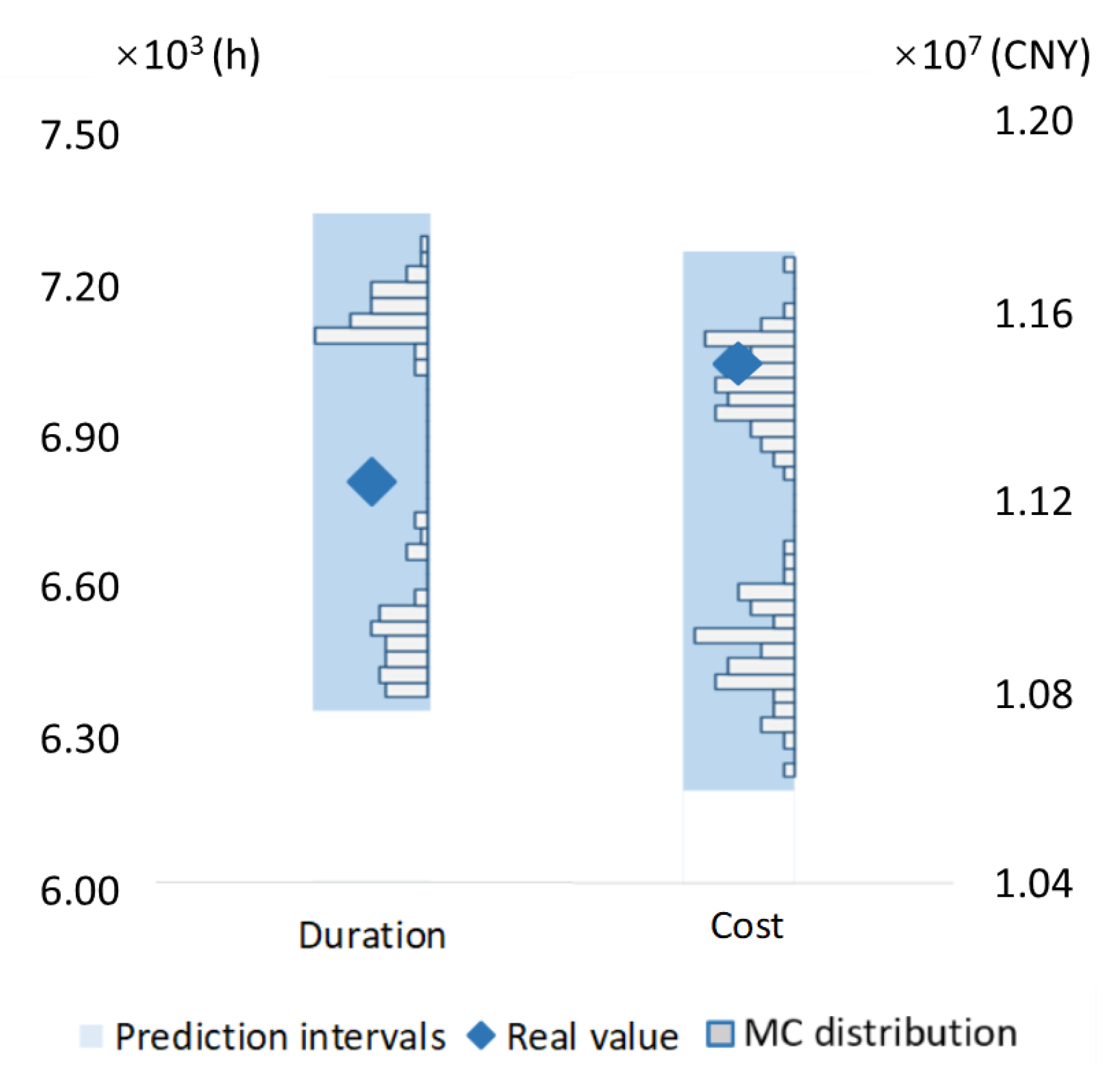
Assess the construction performance by providing prediction intervals for various construction schemes of interest at the planning stage (see Figure 8);

-

Compare numerous schemes at the construction planning stage to identify the best schemes for each specific objective, as well as eliminate schemes that cannot obtain the expected performance (see Figure 9);

-

Reveal the hidden relationships between specific construction parameters for more informed decision making (see Figure 10).

The abilities outlined above mean that the practical contribution of the proposed approach is that it provides the contractor with an effective tool to make informed decisions on construction planning in a situation of deep uncertainty.

6.2. Recommendations and Future Work

Decision making in any construction project is inherently influenced by many sources of uncertainty. This type of problem has already received extensive research attention. However, there is still plenty of room for improvement—for example, a method can handle the construction uncertainty in a more comprehensive way. This research focused on uncertainty within construction planning, i.e., the phase of a project prior to construction execution. An area of research that still needs to be tackled is how project managers can make the right decisions when construction is being operated in a deep uncertainty situation, i.e., the project already starts to construct. This could be relevant with impending climate change, the price fluctuations caused by the COVID-19 pandemic, and other deep uncertain factors that can heavily impact construction execution. Integrating the present research, which primarily concerns the construction at the planning stage, with future work at the execution stage could provide contractors with a comprehensive tool for decision making under deep uncertainty.

References

1. Construction Industry Institute. Front end Planning: Break the Rules, Pay the Price; The University of Texas at Austin: Austin, TX, USA, 2006. [Google Scholar]
2. Lau, S.E.N.; Zakaria, R.; Aminudin, E.; Saar, C.C.; Yusof, A.; Wahid, C.M.F.H.C. A review of application building information modeling (BIM) during pre-construction stage: Retrospective and future directions. IOP Conf. Ser. Earth Environ. Sci. 2018, 143, 012050. [Google Scholar]
3. Moret, Y.; Einstein, H.H. Construction cost and duration uncertainty model: Application to high-speed rail line project. J. Constr. Eng. Manag. 2016, 142, 05016010. [Google Scholar] [CrossRef]
4. Alzraiee, H.; Zayed, T.; Moselhi, O. Dynamic planning of construction activities using hybrid simulation. Autom. Constr. 2015, 49, 176–192. [Google Scholar] [CrossRef]
5. Hong, J.; Shen, G.Q.; Peng, Y.; Feng, Y.; Mao, C. Uncertainty analysis for measuring greenhouse gas emissions in the building construction phase: A case study in China. J. Clean. Prod. 2016, 129, 183–195. [Google Scholar] [CrossRef] [Green Version]
6. Torp, O.; Klakegg, O.J. Challenges in cost estimation under uncertainty: A case study of the decommissioning of Barsebäck Nuclear Power Plant. Adm. Sci. 2016, 6, 14. [Google Scholar] [CrossRef] [Green Version]
7. Ibadov, N.; Kulejewski, J. Construction projects planning using network model with the fuzzy decision node. Int. J. Environ. Sci. Technol. 2019, 16, 4347–4354. [Google Scholar] [CrossRef] [Green Version]
8. Raoufi, M.; Fayek, A.R. Fuzzy Monte Carlo agent-based simulation of construction crew performance. J. Constr. Eng. Manag. 2020, 146, 04020041. [Google Scholar] [CrossRef]
9. Rezakhani, P. Project scheduling and performance prediction: A fuzzy-Bayesian network approach. Eng. Constr. Archit. Manag. 2021, 28, 2233–2244. [Google Scholar] [CrossRef]
10. Sadeghi, N.; Fayek, A.R.; Gerami Seresht, N. A fuzzy discrete event simulation framework for construction applications: Improving the simulation time advancement. J. Constr. Eng. Manag. 2016, 142, 04016071. [Google Scholar] [CrossRef]
11. Rezakhani, P.; Maghiar, M. Fuzzy analytical solution for activity duration estimation under uncertainty. ASCE-ASME J. Risk Uncertain. Eng. Syst. Part A Civ. Eng. 2019, 5, 04019014. [Google Scholar] [CrossRef]
12. Walker, W.E.; Lempert, R.J.; Kwakkel, J.H. Deep Uncertainty. In Encyclopedia of Operations Research and Management Science; Gass, S.I., Fu, M.C., Eds.; Springer: New York, NY, USA, 2013. [Google Scholar]
13. Bryant, B.P.; Lempert, R.J. Thinking inside the box: A participatory, computer-assisted approach to scenario discovery. Technol. Forecast. Soc. Change 2010, 77, 34–49. [Google Scholar] [CrossRef]
14. Beh, E.H.; Zheng, F.; Dandy, G.C.; Maier, H.R.; Kapelan, Z. Robust optimization of water infrastructure planning under deep uncertainty using metamodels. Environ. Model. Softw. 2017, 93, 92–105. [Google Scholar] [CrossRef]
15. Yang, D.Y.; Frangopol, D.M. Risk-based portfolio management of civil infrastructure assets under deep uncertainties associated with climate change: A robust optimisation approach. Struct. Infrastruct. Eng. 2020, 16, 531–546. [Google Scholar] [CrossRef]
16. Khanh, H.D.; Kim, S.Y. A survey on production planning system in construction projects based on Last Planner System. KSCE J. Civ. Eng. 2016, 20, 1–11. [Google Scholar] [CrossRef] [Green Version]
17. Waly, A.F.; Thabet, W.Y. A virtual construction environment for preconstruction planning. Autom. Constr. 2003, 12, 139–154. [Google Scholar] [CrossRef]
18. Project Management Institute. A Guide to the Project Management Body of Knowledge, 5th ed.; Project Management Institute: Newtown Square, PA, USA, 2013. [Google Scholar]
19. Construction Users Roundtable. Collaboration, Integrated Information, and the Project Lifecycle in Building Design, Construction and Operation; The Construction Users Roundtable: Cincinnati, OH, USA, 2004. [Google Scholar]
20. Song, L.; Al-Battaineh, H.T.; AbouRizk, S.M. Modeling uncertainty with an integrated simulation system. Can. J. Civ. Eng. 2005, 32, 533–542. [Google Scholar] [CrossRef]
21. Qie, L.W.; Choi, B.H.; Xie, S.L. Calculation of failure probability of caisson breakwater considering correlation between variables. KSCE J. Civ. Eng. 2009, 13, 1–5. [Google Scholar] [CrossRef]
22. Tegeltija, M.; Oehmen, J.; Kozine, I.; Geraldi, J. Post-Probabilistic Uncertainty Quantification: Discussion of Potential Use in Product Development Risk Management. In Proceedings of the DESIGN 2016 14th International Design Conference, Dubrovnik, Croatia, 16–19 May 2016; pp. 533–542. [Google Scholar]
23. Xiao, X.; Wang, F.; Li, H.; Skitmore, M. Modelling the stochastic dependence underlying construction cost and duration. J. Civ. Eng. Manag. 2018, 24, 444–456. [Google Scholar] [CrossRef] [Green Version]
24. Huijbregts, M.A.; Gilijamse, W.; Ragas, A.M.; Reijnders, L. Evaluating uncertainty in environmental life-cycle assessment. A case study comparing two insulation options for a Dutch one-family dwelling. Environ. Sci. Technol. 2003, 37, 2600–2608. [Google Scholar]
25. Karanki, D.R.; Rahman, S.; Dang, V.N.; Zerkak, O. Epistemic and aleatory uncertainties in integrated deterministic and probabilistic safety assessment: Tradeoff between accuracy and accident simulations. Reliab. Eng. Syst. Saf. 2017, 162, 91–102. [Google Scholar] [CrossRef]
26. Modica, S.; Rustichini, A. Unawareness and partitional information structures. Games Econ. Behav. 1999, 27, 265–298. [Google Scholar] [CrossRef] [Green Version]
27. Shortridge, J.; Aven, T.; Guikema, S. Risk assessment under deep uncertainty: A methodological comparison. Reliab. Eng. Syst. Saf. 2017, 159, 12–23. [Google Scholar] [CrossRef]
28. Feng, K.; Wang, S.; Lu, W.; Liu, C.; Wang, Y. Planning construction projects in deep uncertainty: A data-driven uncertainty analysis approach. J. Constr. Eng. Manag. 2022, 148, 04022060. [Google Scholar] [CrossRef]
29. Marzouk, M.; Elkadi, M. Estimating water treatment plants costs using factor analysis and artificial neural networks. J. Clean. Prod. 2016, 112, 4540–4549. [Google Scholar] [CrossRef]
30. Tatari, O.; Kucukvar, M. Cost premium prediction of certified green buildings: A neural network approach. Build. Environ. 2011, 46, 1081–1086. [Google Scholar] [CrossRef]
31. Wang, Y.-R.; Yu, C.-Y.; Chan, H.-H. Predicting construction cost and schedule success using artificial neural networks ensemble and support vector machines classification models. Int. J. Proj. Manag. 2012, 30, 470–478. [Google Scholar] [CrossRef]
32. Shrestha, D.L.; Solomatine, D.P. Machine learning approaches for estimation of prediction interval for the model output. Neural Netw. 2006, 19, 225–235. [Google Scholar] [CrossRef] [PubMed]
33. Löfgren, B.; Tillman, A.-M. Relating manufacturing system configuration to life-cycle environmental performance: Discrete-event simulation supplemented with LCA. J. Clean. Prod. 2011, 19, 2015–2024. [Google Scholar] [CrossRef]
34. Lu, M. Simplified discrete-event simulation approach for construction simulation. J. Constr. Eng. Manag. 2003, 129, 537–546. [Google Scholar] [CrossRef]
35. Tolk, A.; Turnitsa, C.D. Conceptual modeling of information exchange requirements based on ontological means. In Proceedings of the Winter Simulation Conference, Washington, DC, USA, 9–12 December 2007; pp. 1100–1107. [Google Scholar]
36. Mohamed, Y.; AbouRizk, S. A hybrid approach for developing special purpose simulation tools. Can. J. Civ. Eng. 2006, 33, 1505–1515. [Google Scholar] [CrossRef]
37. Saba, F.; Mohamed, Y. An ontology-driven framework for enhancing reusability of distributed simulation modeling of industrial construction processes. Can. J. Civ. Eng. 2013, 40, 917–926. [Google Scholar] [CrossRef]
38. Fischer, M.; Aalami, F.; Kuhne, C.; Ripberger, A. Cost-loaded production model for planning and control. In Durability of Building Materials and Components; Lacasse, M.A., Vanier, D.J., Eds.; Institute for Research in Construction: Ottawa, ON, Canada, 1999; pp. 2813–2824. [Google Scholar]
39. Zheng, H.; Moosavi, V.; Akbarzadeh, M. Machine learning assisted evaluations in structural design and construction. Autom. Constr. 2020, 119, 103346. [Google Scholar] [CrossRef]
40. Heskes, T. Practical confidence and prediction intervals. Adv. Neural Inf. Process. Syst. 1996, 9, 176–182. [Google Scholar]
41. Heravi, G.; Eslamdoost, E. Applying artificial neural networks for measuring and predicting construction-labor productivity. J. Constr. Eng. Manag. 2015, 141, 04015032. [Google Scholar] [CrossRef]
42. Gao, H.; Qian, X.; Zhang, R.; Ye, R.; Liu, Z.; Qian, Y. Bayesian regularized back-propagation neural network model for chlorophyll-a prediction: A case study in meiliang bay, Lake Taihu. Environ. Eng. Sci. 2015, 32, 938–947. [Google Scholar] [CrossRef]
43. Foresee, F.D.; Hagan, M.T. Gauss-Newton approximation to Bayesian learning. In Proceedings of the International Conference on Neural Networks (ICNN’97), Houston, TX, USA, 9–12 June 1997; pp. 1930–1935. [Google Scholar]
44. Asadi, E.; da Silva, M.G.; Antunes, C.H.; Dias, L.; Glicksman, L. Multi-objective optimization for building retrofit: A model using genetic algorithm and artificial neural network and an application. Energy Build. 2014, 81, 444–456. [Google Scholar] [CrossRef]
45. Bengio, Y. Learning deep architectures for AI. Found. Trends Mach. Learn. 2009, 2, 1–127. [Google Scholar] [CrossRef]
46. Doan, C.D.; Liong, S.-y. Generalization for multilayer neural network bayesian regularization or early stopping. In Proceedings of the Asia Pacific Association of Hydrology and Water Resources 2nd Conference, Singapore, 5–8 July 2004; pp. 5–8. [Google Scholar]
47. MacKay, D.J. Bayesian interpolation. Neural Comput. 1992, 4, 415–447. [Google Scholar] [CrossRef]
48. Huang, H.-C.; Chuang, Y.-Y.; Chen, C.-S. Multiple kernel fuzzy clustering. IEEE Trans. Fuzzy Syst. 2011, 20, 120–134. [Google Scholar] [CrossRef] [Green Version]
49. Tang, A.H.; Cai, L.; Zhang, Y.M. Application of hard C-means and fuzzy C-means in data fusion. Appl. Mech. Mater. 2012, 190, 265–268. [Google Scholar] [CrossRef]
50. Tsai, D.-M.; Lin, C.-C. Fuzzy C-means based clustering for linearly and nonlinearly separable data. Pattern Recognit. 2011, 44, 1750–1760. [Google Scholar] [CrossRef]
51. Dunn, J.C. A fuzzy relative of the ISODATA process and its use in detecting compact well-separated clusters. J. Cybern. 1973, 3, 32–57. [Google Scholar] [CrossRef]
52. Bezdek, J.C. Pattern Recognition with Fuzzy Objective Function Algorithms; Plenum Press: New York, NY, USA, 2013. [Google Scholar]
53. Solomatine, D.P.; Siek, M.B. Modular learning models in forecasting natural phenomena. Neural Netw. 2006, 19, 215–224. [Google Scholar] [CrossRef] [PubMed]
54. Elbeltagi, E.; Hegazy, T.; Grierson, D. Comparison among five evolutionary-based optimization algorithms. Adv. Eng. Inform. 2005, 19, 43–53. [Google Scholar] [CrossRef]
55. Li, S.; Fan, Z. Evaluation of urban green space landscape planning scheme based on PSO-BP neural network model. Alex. Eng. J. 2022, 61, 7141–7153. [Google Scholar] [CrossRef]
56. Feng, K.; Lu, W.; Wang, Y. Assessing environmental performance in early building design stage: An integrated parametric design and machine learning method. Sustain. Cities Soc. 2019, 50, 101596. [Google Scholar] [CrossRef]
57. Heaton, J. The Number of Hidden Layers. Available online: https://www.heatonresearch.com/2017/06/01/hidden-layers.html (accessed on 26 December 2022).
58. LeCun, Y.; Bengio, Y.; Hinton, G. Deep learning. Nature 2015, 521, 436–444. [Google Scholar] [CrossRef]
59. Shanghai Wind Chaser Team. Overview of Typhoon in Guangdong Province. Available online: http://www.stwc.icoc.cc/h-col-175.html (accessed on 9 April 2022). (In Chinese).
60. Tam, V.W.; Shen, L.; Tam, C.M. Assessing the levels of material wastage affected by sub-contracting relationships and projects types with their correlations. Build. Environ. 2007, 42, 1471–1477. [Google Scholar] [CrossRef] [Green Version]
61. Al-Hajj, A.; Hamani, K. Material waste in the UAE construction industry: Main causes and minimization practices. Archit. Eng. Des. Manag. 2011, 7, 221–235. [Google Scholar] [CrossRef]
62. Zhang, H.; Yu, L. Dynamic transportation planning for prefabricated component supply chain. Eng. Constr. Archit. Manag. 2020, 27, 2553–2576. [Google Scholar] [CrossRef]
63. Tucker, R.L. Management of construction productivity. J. Manag. Eng. 1986, 2, 148–156. [Google Scholar] [CrossRef]
64. Construction Engineering Cost Management Station Shenzhen. Construction Engineering Quota of Shenzhen; China Building Industry Press: Shenzhen, China, 2016. (In Chinese) [Google Scholar]
65. MOHURD. Construction Equipment Engineering Quota of China; Ministry of Housing and Urban-Rural Development: Beijing, China, 2012.
66. Banks, J. Handbook of Simulation: Principles, Methodology, Advances, Applications, and Practice; John Wiley & Sons: Hoboken, NJ, USA, 1998. [Google Scholar]
67. Wilcoxon, F. Individual Comparisons by Ranking Methods. In Breakthroughs in Statistics; Springer: New York, NY, USA, 1992; pp. 196–202. [Google Scholar]
68. Imam, A.; Usman, M.; Chiawa, M.A. On Consistency and limitation of paired t-test, Sign and Wilcoxon Sign Rank Test. IOSR J. Math. 2014, 10, 1–6. [Google Scholar] [CrossRef]
69. Wang, Y.; Feng, K.; Lu, W. An environmental assessment and optimization method for contractors. J. Clean. Prod. 2017, 142, 1877–1891. [Google Scholar] [CrossRef]
70. Lee, S.; Han, S.; Peña-Mora, F. Integrating construction operation and context in large-scale construction using hybrid computer simulation. J. Comput. Civ. Eng. 2009, 23, 75–83. [Google Scholar] [CrossRef]
71. Li, C.Z.; Xu, X.; Shen, G.Q.; Fan, C.; Li, X.; Hong, J. A model for simulating schedule risks in prefabrication housing production: A case study of six-day cycle assembly activities in Hong Kong. J. Clean. Prod. 2018, 185, 366–381. [Google Scholar] [CrossRef]
72. Feng, K.; Chen, S.; Lu, W.; Wang, S.; Yang, B.; Sun, C.; Wang, Y. Embedding ensemble learning into simulation-based optimisation: A learning-based optimisation approach for construction planning. Eng. Constr. Archit. Manag. 2021. [Google Scholar] [CrossRef]
73. Lee, J.-S.; Filatova, T.; Ligmann-Zielinska, A.; Hassani-Mahmooei, B.; Stonedahl, F.; Lorscheid, I.; Voinov, A.; Polhill, J.G.; Sun, Z.; Parker, D.C. The complexities of agent-based modeling output analysis. J. Artif. Soc. Soc. Simul. 2015, 18. [Google Scholar] [CrossRef]
74. Uusitalo, L.; Lehikoinen, A.; Helle, I.; Myrberg, K. An overview of methods to evaluate uncertainty of deterministic models in decision support. Environ. Model. Softw. 2015, 63, 24–31. [Google Scholar] [CrossRef] [Green Version]
75. Muthén, L.K.; Muthén, B.O. How to use a Monte Carlo study to decide on sample size and determine power. Struct. Equ. Model. 2002, 9, 599–620. [Google Scholar] [CrossRef]
Figure 1. Schematic illustration of uncertainty and the influence of decisions throughout the project life cycle, adapted from the Project Management Institute [18] and MacLeamy Curve [19].
Buildings 13 00254 g001
Figure 2. A flowchart of the presented prediction intervals modeling approach for construction planning.
Buildings 13 00254 g002
Figure 3. The creation of a DES model for construction process simulation.
Buildings 13 00254 g003
Figure 4. The structure of the BRBNN model for baseline prediction.
Buildings 13 00254 g004
Figure 5. The process of the standard floor construction.
Buildings 13 00254 g005
Figure 6. Duration modeling with different sample sizes and optimization settings: (a) Pareto front obtained with different sample sizes; (b) Pareto front obtained with the optimal sample size.
Buildings 13 00254 g006
Figure 7. Cost modeling with different sample sizes and optimization settings: (a) Pareto front obtained with different sample sizes; (b) Pareto front obtained with the optimal sample size.
Buildings 13 00254 g007
Figure 8. Construction performance prediction intervals for testing samples: (a) Testing for project duration; (b) Testing for project cost.
Buildings 13 00254 g008
Figure 9. The mean values and prediction intervals of the project performance for various samples.
Buildings 13 00254 g009
Figure 10. Effect of labor force on the project duration and the level of uncertainty: (a) Project duration; (b) Uncertainty level.
Buildings 13 00254 g010
Figure 11. A comparison of the prediction intervals and actual values for project duration and cost.
Buildings 13 00254 g011