A Method for Predicting the Corrosion Behavior of Structural Steel under Atmosphere

Abstract

The durability and safety of steel structures during their life cycle are affected by steel corrosion. Limited test conditions and time hinder the reproduction of actual atmospheric steel corrosion. Most test studies have focused on the effect of pitting or uniform corrosion of steel structures, leading to the development of vague engineering methods that make it difficult to design steel structures with excellent corrosion resistance. In this study, a method involving three-dimensional cellular automata and a genetic algorithm was developed for predicting the corrosion behavior of structural steel. The calculation efficiency of three-dimensional cellular automata was improved by small iterative steps and adaptive activation for potential corrosion. Furthermore, the proposed method was tested with published tests, and the results showed that the method can simulate atmospheric corrosion with excellent accuracy and efficiency. The simulation results were used to calculate the structural steel cross-sectional performance with greater accuracy than that of the method of assuming uniform corrosion. Meanwhile, with accurate material parameters, the proposed method can also simulate the atmospheric corrosion of high-performance steel of different strengths and properties.

1. Introduction

When the surface protective material of structural steel is damaged, the steel becomes corroded by water ions in the atmosphere, as shown in Figure 1 [1]. Corrosion is a common structural defect that reduces the bearing capacity of structures [2,3]. The corrosion of structural steel is stochastic and non-uniform, unlike the generalized external force. Currently, the lack of experimental conditions and steel morphology corrosion data makes it difficult to simulate the actual corrosion process of steel. Most studies have only investigated and simulated the uniform corrosion [4,5,6] and spot corrosion [7,8,9] of structural steel.

The uniform corrosion of structural steel can be simulated locally or comprehensively by uniformly weakening the cross-sectional area of the steel structure, but the method ignores the impact of non-uniform corrosion, such as pitting corrosion, on the steel strength [10,11,12,13]. The manual drilling test or finite element software can also be used to analyze the relationship between the strength of the steel components’ and stochastic pitting corrosion [14,15,16,17,18]. However, the test and software ignore the pitting shape randomness and the real atmospheric environment cannot be simulated accurately, and there is still a gap between the state under atmospheric corrosion conditions. Meanwhile, the accuracy of steel corrosion simulations performed through artificial accelerated corrosion tests need to be verified [19,20,21,22,23,24], and further investigations are required for the relationship between the test results and corrosion under natural atmospheric conditions. Thus, the simulated accelerated corrosion test cannot replace the atmospheric corrosion test under current conditions [25]. Most existing natural atmospheric corrosion tests are old, and advanced instruments cannot be used to determine the corrosion surface characteristics. The load-bearing method is commonly used here to obtain the average corrosion depth for characterizing corrosion, but performing repeated tests to study the corrosion surface characteristics is time-consuming and incurs high equipment costs.

Cellular automata (CA) have been used for corrosion simulation [26] in many studies, such as [27,28], and high-temperature corrosion and intergranular corrosion have been predicted by CA. The use of two-dimensional CA for simulating steel corrosion [29,30,31] is inadequate for the three-dimensional world. Although three-dimensional CA without mathematical constraints can be used to simulate steel corrosion, it is difficult to calculate the optimal independent variable parameters because of simulation error [32,33,34].

In addition, current research on the degradation resistance model is mainly focused on concrete members; little attention has been directed toward the degradation resistance of steel members to corrosion under atmospheric conditions. Owing to the difficulty of obtaining the surface morphology of corroded steel, only a few studies [35,36] have investigated the degradation resistance law of steel components by assuming uniform corrosion; however, these studies did not sufficiently consider the randomness and irregularity of corrosion [37].

With the recent rise of artificial intelligence algorithms such as machine learning, AI technology has also been applied to steel corrosion analysis and other technical fields. Studies such as [38,39] examined the effectiveness of AI algorithms for the prediction of the internal corrosion rate for oil and gas pipelines in complex environments and the corrosion rate in main cables of suspension bridges were described respectively. The results showed that AI algorithms can effectively predict steel corrosion in complex environments. However, the prediction of structural steel corrosion with an AI-based framework needs a huge database, which is difficult to obtain. Limited by the steel corrosion stochastic, most measured and tested data are highly discrete, and it is difficult for AI to judge the validity of this data. As a result, if the database is too small, AI simulation results are easily unfaithful.

In this study, with the assumption that the structural steel’s average corrosion depth is the same within the region, steel surface morphology obtained by combining CA and a genetic algorithm (GA) was used to develop a method for determining the properties of the steel sections. The data used were obtained from a published atmospheric corrosion database, and steel corrosion under atmospheric conditions was simulated. Optimal corrosion parameters were obtained by optimizing the simulation error. The major contributions of this study are as follows:

(1)

The results provide a basis for calculating stiffness and for precise finite element analysis, considering the randomness of corrosion.

(2)

Our method can be used for calculating structural time-based reliability and optimizing the service life of steel structures.

(3)

The study provides a method for the experimental study of corrosion mechanisms.

2. Corrosion Simulation Analysis Based on CA-GA

2.1. Simulation Error Evaluation Method

Two classic tests have been proposed in previous research on the atmospheric corrosion of steel:

Liang [40] conducted 16-year atmospheric corrosion tests of steel in several representative regions of China and converted the weight loss into the average corrosion depth. The author assumed uniform corrosion in the study and found that the relationship between corrosion depth and time is as expressed in Equation (1),

$$D=A\cdot t^n,$$

(1)

where D is the average corrosion depth (mm), t is the duration of the steel exposure to the atmosphere (y), and A and n are constants. For A3 structural steel with a nominal yield strength of 235 MPa, the statistical test results of A and n in some representative regions of China are expressed in

Table 1. Statistical values of A and n in representative regions of China.

City	Beijing	Guangzhou	Qingdao	Chongqing	Wuhan
A	0.030	0.056	0.057	0.074	0.049
n	0.420	0.41	0.61	0.41	0.24
Type of atmosphere	Normal	Normal	Offshore	Normal	Normal

.

Xiao [41] conducted natural exposure and indoor accelerated tests under general atmospheric and offshore atmospheric conditions for steel plate with a nominal yield strength of 235 MPa. The average non-uniform corrosion depth was proposed as an evaluation parameter of surface morphology to represent the distance between the comprehensive corrosion plane and the non-uniform corrosion. According to the test results, the average non-uniform corrosion depth under general atmospheric conditions was expressed as Δt_ave = 3.0Δt_e^0.67; the average non-uniform corrosion depth under offshore atmospheric conditions was Δt_ave = 3.48Δt_e^0.64. Δt_e represents the equivalent corrosion thickness, which has the same meaning as the average corrosion depth D in tests [40]. A combination of the average corrosion depth and non-uniform corrosion depth enables the assessment of the degree of general corrosion and the degree of non-uniform corrosion. Therefore, we created the CA-GA algorithm in this study. The CA algorithm was first used to simulate the atmospheric corrosion of steel with different input parameters, and the calculation results of the average corrosion depth and average non-uniform corrosion depth under different input parameters were obtained. The relative error of the simulation results was then calculated using Equation (2):

$$D_{\mathrm{m}}=\frac{1}{NM}{\displaystyle \sum _{i=1}^N{\displaystyle \sum _{j=1}^{M}d(x_i,y_j)}},$$

(2)

$$Er(D)=\frac{D_{\mathrm{m}}-D}{D},$$

(3)

$$\Delta t{m}_{\mathrm{ave}}=\frac{1}{NM}{\displaystyle \sum _{i=1}^N{\displaystyle \sum _{j=1}^{M}d(x_i,y_j)}}-D_{\mathrm{mp}},$$

(4)

$$Er(\Delta t_{\mathrm{ave}})=\frac{\Delta t{m}_{\mathrm{ave}}-\Delta t_{\mathrm{ave}}}{\Delta t_{\mathrm{ave}}},$$

(5)

where d (x_i, y_i) indicates the atmospheric corrosion depth corresponding to the coordinates in the CA model; D_m refers to the average simulated corrosion depth; D is the average test corrosion depth; N and M refer to the number of cells of the CA model in the x and y axes, respectively; and Er(D) refers to the relative error of the average corrosion depth simulation results. Furthermore, Δtm_ave indicates the atmospheric corrosion depth corresponding to the coordinates in the CA model; D_mp refers to the simulated average corrosion depth; Δt_ave is the average test corrosion depth; a and b refer to the number of cells of the CA model in the x and y axes, respectively. Er (Δt_ave) refers to the relative error of the simulated average non-uniform corrosion depth.

The GA algorithm was then used to obtain the average value of the simulation errors of the two indicators as a basis for calculating the fitness value. The input parameters were optimized to minimize the simulation errors of the two indicators. The calculation method of the fitness value was expressed as follows:

$$fin=\frac{1}{\overline{Er}}=\frac{1}{{\displaystyle \sum _{i=1}^{W}E{r}_i}}=\frac{1}{{\displaystyle \sum _{i=1}^W\left(\frac{\left|Er(D_i)\right|+\left|Er(\Delta t_{\mathrm{ave},i})\right|}{2}\right)}},$$

(6)

where fin represents the fitness value; W represents the number of repeated CA simulations; Er_i, Er(D_i), and Er (Δt_ave, i) represent the comprehensive error of the i-th CA simulation, the relative error of the average corrosion depth, and the relative error of the average non-uniform corrosion depth, respectively. $\overline{Er}$ represents the average value of the comprehensive error of W repeated CA simulations; W = 10 in this study. Using optimized input parameters for the CA algorithm yielded a reasonable simulation of the atmospheric corrosion of steel.

2.2. Definition and Evolution Rules of Cellular Automata (CA)

2.2.1. Definition of CA

CA selects several cellular units to form a cellular space. In each iteration step, each cellular unit is influenced by the state of the neighboring cells and updates its own state according to certain evolution rules. Here, we selected the Moore neighborhood [42]: the state of each cell unit is affected by the surrounding six cell units, as illustrated in Figure 2a. Owing to the limited size of the cell space, boundary conditions should be set outside the cell space to effectively simulate the infinite space with the finite space. Periodic boundary conditions were selected in this study, as illustrated in Figure 2b: the blue cell unit represents the unit outside the boundary and the green cell unit is the unit within the boundary. The periodic boundary connects the edge units of the CA, which is the most suitable boundary form for infinite space.

We selected 104 × 104 × 104 cell units as the initial research object; the outermost two layers of cells were the periodic boundaries, and the initial side length of the cell unit was d₀ = 0.01 mm. An unspecified time was used as the iterative step, and an iterative mechanism combining large and small iterative steps was developed. One year was used as the time unit of a large iterative step and each large iterative step comprised smaller iterative steps. When the average corrosion depth simulation value corresponding to the large iteration step was fitted to the test results of the average corrosion depth of the year, the iteration stopped, and the average non-uniform corrosion depth was calculated accordingly. To fully consider the randomness of the CA simulation, 10 CA simulations were performed simultaneously for each year (large iteration). The cell matrix with the smallest simulation error was used as the cell matrix at the beginning of the next large iteration. According to the definition of evolution rules [32,33], we defined the evolution rules of cell units as c_t+1 = c_t(M_1,2, W, CM, P), where c represents a cell unit, t represents a small iterative step, M_1,2 represents a metal unit, W represents a water unit, CM represents medium units, W and CM are collectively referred to as non-metallic state cell units, and the corrosion medium concentration w_c represents the ratio of the number of corrosion medium units to the number of non-metallic units:

$$w_{\mathrm{c}}=\frac{{\displaystyle {\sum }_{i}CM}}{{\displaystyle {\sum }_{i}W}+{\displaystyle {\sum }_{i}CM}},$$

(7)

At the beginning of each small iterative step, each M₀ randomly becomes either W or CM according to the value of w_c. Metal cells exist in two states: unpassivation state M₁ and passivation state M₂.

P represents probability. Following [29,32,33], corrosion probability and passivation probability, the simulated corrosion and passivation processes were considered, and the passivation product was assumed as never damaged, which was inconsistent with the actual situation. Therefore, the passivation film rupture probability was added as the input parameter of the CA to consider the actual situation of the passivation film damage due to factors such as rain erosion. Probability P = P_c + P_p + P_n + P_b = 1, where P_c represents corrosion probability, P_p represents passivation probability, P_b represents passivation film rupture probability, P_n represents the probability of no event, and the four events are mutually exclusive. In each small iteration step, the probability P has four likely situations:

(1)

If a corrosive medium is in the neighboring unit of an unpassivation metal cell unit M₁, the corresponding P_b of the cell unit is 0 and P_c, P_p, P_n ≠ 0. The essence is that when a corrosive medium is around the metal without passivation, corrosion, passivation, or no chemical reaction occurs, but a passivation film rupture does not occur.

(2)

If no corrosive medium is in the neighboring unit of an unpassivation metal cell unit M₁, the corresponding probability of the cell unit is P_b = P_c = P_p = 0. The essence is that when no corrosive medium is around the metal without passivation, corrosion, passivation, and passivation film rupture do not occur; at this time, P = P_n = 1.

(3)

The probability corresponding to the passivation state cell unit M₂ is P_c = P_p = 0 and P_b, P_n ≠ 0. The essence is that the metal in the passivation state does not undergo corrosion and repeated passivation, but passivation film rupture may occur. It is also possible that no chemical reaction occurs.

(4)

The probability corresponding to the non-metallic cell unit M₀ is P_b = P_p = P_c = 0. The essence is that the non-metallic cell unit does not undergo a chemical reaction; at this time, P = P_n = 1.

2.2.2. Definition of Evolution Rules

The iterative state of the cell state M is as follows:

$M_2^{t+1}=M_1^t|P_{\mathrm{p}}$, where $M_1^t$ represents the unpassivation metal state cell in the t-th small iterative step, $M_1^t|P_{\mathrm{p}}$ represents passivation occurring in the cell, and $M_2^{t+1}$ represents the passivation metal state cell in the (t + 1)-th small iterative step. The whole process represents the passivation of unpassivation metal state cells to passivation metal state cells.

$M_1^{t+1}=M_2^t|P_{\mathrm{b}}$, where $M_2^t$ represents the passivation metal state cell in the t-th small iterative step, $M_2^t|P_{\mathrm{b}}$ represents the passivation film rupture event in this cell, and $M_1^{t+1}$ represents the unpassivation metal state cell in the (t + 1)-th small iterative step. The whole process indicates that the passivation film of the passivation metal state cell is broken, and the cell unit is transformed into an unpassivation metal state cell unit.

$M_2^{t+1}=M_2^t|\overline{P_{\mathrm{b}}}$, where $M_2^t$ represents the passivation metal state cell in the t-th small iterative step, $M_2^t|\overline{P_{\mathrm{b}}}$ indicates that the passivation film rupture event does not occur in this cell, and $M_2^{t+1}$ represents the passivation metal state cell in the (t + 1)-th small iterative step. The whole process means that if the passivation metal state cell lacks a passivation film rupture event, the existing state is maintained.

$M_0^{t+1}=M_1^t|P_{\mathrm{c}}$, where $M_1^t$ represents the unpassivation metal state cell in the t-th small iteration step, $M_1^t|P_{\mathrm{c}}$ represents the corrosion event in the cell, and $M_0^{t+1}$ represents the non-metallic state cell in the (t + 1)-th small iterative step. The whole process indicates that the unpassivation metal state cell undergoes corrosion and transforms into a non-metallic state cell.

$M_1^{t+1}=M_1^t|\overline{P_{\mathrm{c}}}$, where $M_1^t$ represents the unpassivation metal state cell in the t-th small iterative step, $M_1^t|\overline{P_{\mathrm{c}}}$ indicates that no corrosion event occurs in the cell, and $M_1^{t+1}$ represents the unpassivation metal state cell in the (t + 1)-th small iterative step. The whole process indicates that the unpassivation metal state cell lacks a corrosion event and remains in its existing state.

If a metal state cell unit is surrounded by non-metal state cells, the cell unit becomes a non-metal state cell unit in the next iteration, thereby simulating the shedding phenomenon.

The cell matrix is obtained by the above method, and the coordinates of the cell unit and the corrosion depth are converted:

$$s(x_i,y_j)=\min (z|c(x_i,y_j)=1,2)-1,$$

(8)

$$d(x_i,y_j)=l\cdot s(x_i,y_j),$$

(9)

where s(x_i, y_i) represents the depth corresponding to coordinate (x_i, y_i), z|_{c(xi, yj)=1,2} represents the z-coordinate value of the metal state or passivation state cell unit (the cell unit state value is 1 or 2), min (z|_{c(xi, yj)=1,2}) is the depth unit value of the shallowest metal or passivation state cell corresponding to the coordinate (x_i, y_i), l indicates the cell unit side length. Following Equations (2)–(5), the GA algorithm was used to optimize the input parameters.

2.2.3. Parameter Interval Setting

(1)

CA input parameter setting:

Different methods for setting parameter intervals have been proposed for similar CA models. In Ref. [29], the passivation probability and corrosion probability interval were set as (0, 1), and the passivation probability was set to be less than the corrosion probability. In Ref. [32], the corrosion probability was set as [0.2, 0.8] and the passivation probability as [0.005, 0.01]. In Ref. [43], the corrosion probability was set as (0, 1); rather than setting the passivation probability, the corrosion probability was adjusted to 0 at a certain number of corrosion pits to achieve the effect of passivation. Assuming that the concentration of the corrosive medium is a constant (as in Refs. [29,32,43]) does not represent the reality of the dynamic nature of the concentration of the corrosive medium under atmospheric corrosion conditions; it also does not consider the phenomenon of passivation film cracking. Because the GA algorithm was used in this study to find the optimal solution of the CA input parameters, the value ranges of the passivation probability P_p, passivation film rupture probability P_b, corrosion probability P_c, and corrosion medium concentration w_c were selected as the largest interval (0, 1). This selection ensured that the optimal value was included in the interval. Meanwhile, the passivation probability was set to be less than the corrosion probability to ensure that the corrosion phenomenon continued.

(2)

GA control parameter setting:

Using the binary coding method, the chromosome structure was as follows:

$$A=a1,a2,\dots ,a9|b1,b2,\dots ,b9|c1,c2,\dots ,c9|d1,d2,\dots ,d9.$$

Chromosomal locations a1-a9 were used to code the corrosion medium concentration w_c, b1 to b9 coded the passivation probability P_p, c1 to c9 coded the corrosion probability P_c, and d1to d9 coded the passivation film rupture probability P_b. In the initial population stage, 10 individuals with a length of 36 were randomly generated; in the selection stage, the roulette method was used, and the generation gap was G = 0.8. The method of single-point crossover was used, and the crossover probability was P_x = 0.7. The method of single-point mutation was used, and the probability of mutation was P_m = 0.7. We set the maximum number of generations to 200.

2.3. Algorithm Iterative Control Mechanism

2.3.1. Cell Fission Mechanism

The function of the average corrosion depth to be fitted in this study was a power function with decreasing increments. As the size of the cell unit of the traditional CA is fixed, in the later stage of the corrosion simulation, the increment of the simulation value of the average corrosion depth in each iteration step is higher than the increment of the average test corrosion depth value in each year [44,45]. Hence, the simulation errors become larger as the erosion time increases. If the size of the cell unit is adjusted to a smaller value, the problem of the later simulation errors can be solved. However, each CA model needs numerous iterations in the early stage of the corrosion simulation; typically, hundreds of small iteration steps are required for a one-year simulation. In addition, the three-dimensional CA model is relatively complex, and after the GA is superimposed, the number of iterations needs to be multiplied by the number of iterations of the GA, which is time-consuming. Hence, we propose a cellular fission mechanism.

The cell fission mechanism causes cell fission when the comprehensive error of the simulation result exceeds a certain limit value according to the simulation situation of the comprehensive error. Each cell unit is divided into two parts along the x, y, and z axes, so that each cell unit becomes eight identical cell units. Meanwhile, the number of iterations of the GA is reset to zero, and the calculation is restarted, thereby improving the simulation accuracy. This approach adaptively adjusts the size of the iteration step and increases the number of iterations when the operation does not converge; consequently, the increment of each iteration step is reduced. The process is as follows:

(1)

Select the side length of the starting cell unit as d₀.

(2)

Start the CA simulation and calculate the errors of the corrosion rate and the average non-uniform corrosion depth.

(3)

When the GA reaches the specified number of operations, if the average error of the two indicators of corrosion rate and average non-uniform corrosion depth meets the requirements, the operation ends; otherwise, each initial cell of the large iteration step is split into eight cells of equal size, and Step (2) is repeated.

2.3.2. Activation Mechanism of Potential Corrosion Area

Owing to the large scale of the CA matrix and the combination of the GA, the number of iterations was large. Taking the corrosion simulation of the first year in Guangzhou as an example, it took more than 8.8 × 10⁶ iterations to perform the corrosion simulation for one year, which was extremely time-consuming. It took more than six days to complete the calculation using a computer with an Intel (R) Core (TM) i5-10210U CPU @ 1.60 GHz, 2.11 GHz, and 16.0 GB of RAM. Therefore, we proposed an activation mechanism for potential corrosion regions.

Naturally, the internal part of steel does not undergo chemical reactions because it is not in contact with the corrosive medium. Current corrosion research using the three-dimensional CA model includes the internal part of the cell units in the iterative calculation. This consideration results in a large number of useless iterations, increasing the time cost. Our proposed activation mechanism for the potential corrosion region activates the region that may undergo chemical action to make it iterative, whereas other parts do not undergo iterative calculation. The process is detailed as follows.

At the beginning of each large iteration, the maximum corrosion depth t (the unit is the side length of one cell unit) is searched for, and the area below the maximum corrosion depth is closed. Because each small iterative step increases the maximum corrosion depth by at most one unit, let t = t + 1 at the beginning of the next small iterative step. The regions with depths greater than t are turned off, and the potential corrosion regions with depths less than or equal to t are activated. Consequently, the computing efficiency is considerably improved. In the first year of the corrosion simulation in Guangzhou, the computing time was shortened from 6 days to 7 h under the same computing environment, which is a 20-fold increase in efficiency.

2.4. CA-GA Algorithm Running Steps

According to the above rule and process definitions of the CA-GA algorithm, combined with the improvement mechanism proposed above, the running steps of the CA-GA algorithm for atmospheric corrosion simulation were as follows:

(1)

Select specific CA parameters such as concentration of corrosive medium, corrosion probability, passivation probability, and passivation film rupture probability to initialize the population.

(2)

According to the CA parameters, each individual activates the potential corrosion area following the CA model simulating atmospheric corrosion in the previous year, and iterates until the average corrosion depth exceeds the target average corrosion depth for the first time.

(3)

Calculate the fitness function value of each individual in the population.

(4)

Select several individuals for crossover and mutation operations, perform Steps (2) and (3) on the chromosome again, and use the roulette method to select a specific number of optimal individuals to replace the worst individual of the parent generation.

(5)

Repeat Steps (2) to (4); if the $\overline{Er}$ of the optimal individual within the maximum generational number is less than the set value (3% in this study), the iteration is terminated, and the optimal solution of the input parameters and the corresponding CA simulation results are output. If the $\overline{Er}$ of the optimal individual with the maximum generational number is greater than the set value, the CA matrix of the previous year undergoes fission, the generational number is cleared, and Steps (1) to (4) are repeated.

The block diagram of the algorithm is shown in Figure 3.

3. Analysis of Atmospheric Corrosion Simulation Results

3.1. Visualization of Simulation Results

To visualize the CA simulation results, we used the grid data function of Matlab to smooth the CA data and the mesh function to create the plots. The corrosion simulation results of the Guangzhou area for time t = 1, 4, 8, and 16 years are illustrated in Figure 4.

In Figure 4, the initial uncorroded plane is the origin of the z direction, while the downward corrosion is the negative part, representing the surface morphology of the corroded steel. Similarly, the x- and y- axes correspond to the coordinates of the cell matrix in the x-y plane. Each length unit is a cell side length. As the cell did not undergo fission in t = 1–8 years, the x-y plane was a matrix with an area of 100 × 100 unit cell; when t = 9–14 years, the first fission occurred, and the matrix area became a 200 × 200 unit cell. The second fission occurred in t = 15~16 years, and the matrix area became a 400 × 400 unit cell.

3.2. Error Analysis of Simulation Results

For five representative cities, including Beijing, Guangzhou, Chongqing, Qingdao, and Wuhan, atmospheric corrosion simulations were performed for 16 years. The simulation errors of the average corrosion depth and the average non-uniform corrosion depth are presented in

Table 2. Statistics of atmospheric corrosion simulation errors in representative areas.

Corrosion Time	Beijing		Guangzhou		Chongqing		Qingdao		Wuhan
	$\mathit{E}\mathit{r}(\mathit{D})$	$\mathit{E}\mathit{r}(\mathbf{\Delta }{\mathit{t}}_{\mathbf{ave}})$	$\mathit{E}\mathit{r}(\mathit{D})$	$\mathit{E}\mathit{r}(\mathbf{\Delta }{\mathit{t}}_{\mathbf{ave}})$	$\mathit{E}\mathit{r}(\mathit{D})$	$\mathit{E}\mathit{r}(\mathbf{\Delta }{\mathit{t}}_{\mathbf{ave}})$	$\mathit{E}\mathit{r}(\mathit{D})$	$\mathit{E}\mathit{r}(\mathbf{\Delta }{\mathit{t}}_{\mathbf{ave}})$	$\mathit{E}\mathit{r}(\mathit{D})$	$\mathit{E}\mathit{r}(\mathbf{\Delta }{\mathit{t}}_{\mathbf{ave}})$
1	0.05%	−0.10%	0.73%	−0.15%	0.18%	−0.09%	0.65%	0.65%	0.17%	0.06%
2	0.02%	0.39%	0.86%	1.03%	0.40%	0.54%	0.28%	0.27%	0.07%	0.98%
3	0.17%	0.47%	0.22%	0.25%	0.10%	0.63%	0.25%	0.26%	0.12%	−0.01%
4	0.04%	0.29%	0.08%	0.24%	0.04%	0.05%	0.34%	0.15%	0.12%	−0.07%
5	0.09%	0.02%	0.16%	0.00%	0.89%	0.37%	1.51%	1.47%	0.00%	0.96%
6	0.21%	−0.14%	0.23%	−0.02%	0.71%	1.08%	0.41%	1.29%	0.26%	0.06%
7	0.37%	0.38%	0.06%	0.16%	0.04%	0.22%	0.13%	−0.09%	0.01%	0.08%
8	0.22%	−0.33%	0.54%	1.07%	0.14%	−0.07%	0.81%	0.60%	0.06%	−0.06%
9	0.02%	0.22%	0.02%	−0.19%	0.18%	−0.15%	0.12%	0.03%	0.93%	0.43%
10	0.02%	0.59%	0.00%	0.69%	0.02%	0.14%	0.07%	0.25%	0.03%	0.26%
11	0.03%	0.20%	0.16%	−0.02%	0.05%	0.11%	0.10%	1.42%	0.02%	0.88%
12	0.08%	−0.19%	0.13%	−0.02%	0.02%	0.64%	0.12%	1.68%	0.07%	1.44%
13	0.13%	−0.02%	0.02%	0.03%	0.04%	−0.03%	0.13%	1.17%	0.95%	−1.75%
14	0.03%	−0.55%	0.01%	0.39%	0.03%	−0.03%	0.13%	2.49%	0.87%	−1.19%
15	0.02%	−0.54%	0.01%	−0.45%	0.06%	−0.16%	1.28%	2.25%	1.11%	−1.57%
16	0.01%	−0.03%	0.02%	−0.05%	0.06%	0.00%	1.98%	2.58%	1.03%	−0.66%

.

It can be seen from Table 2 that Er (D) and Er (Δt_ave) in all regions was less than 3% within 16 years.

3.3. Accuracy Improvement of Fission Mechanism

To examine the effect of the proposed fission mechanism on accuracy improvement, Guangzhou was taken as an example. The traditional CA was combined with a GA, with and without a fission mechanism. The comprehensive errors (mean values of Er (D) and Er (Δt_ave)) of the calculation results are illustrated in Figure 5.

4. Generalized Resistance Degradation of Steel Members under Atmospheric Corrosion Conditions

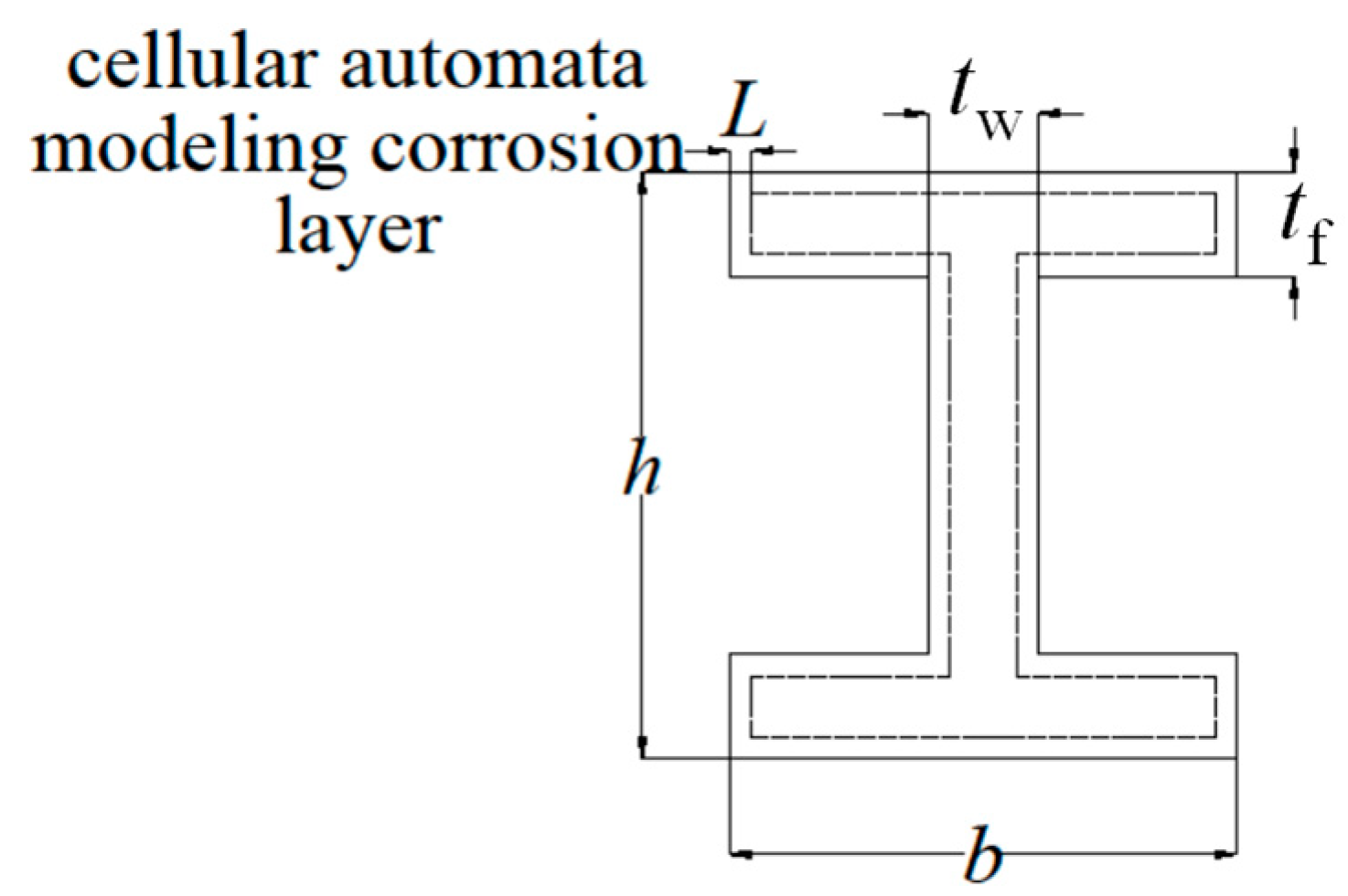
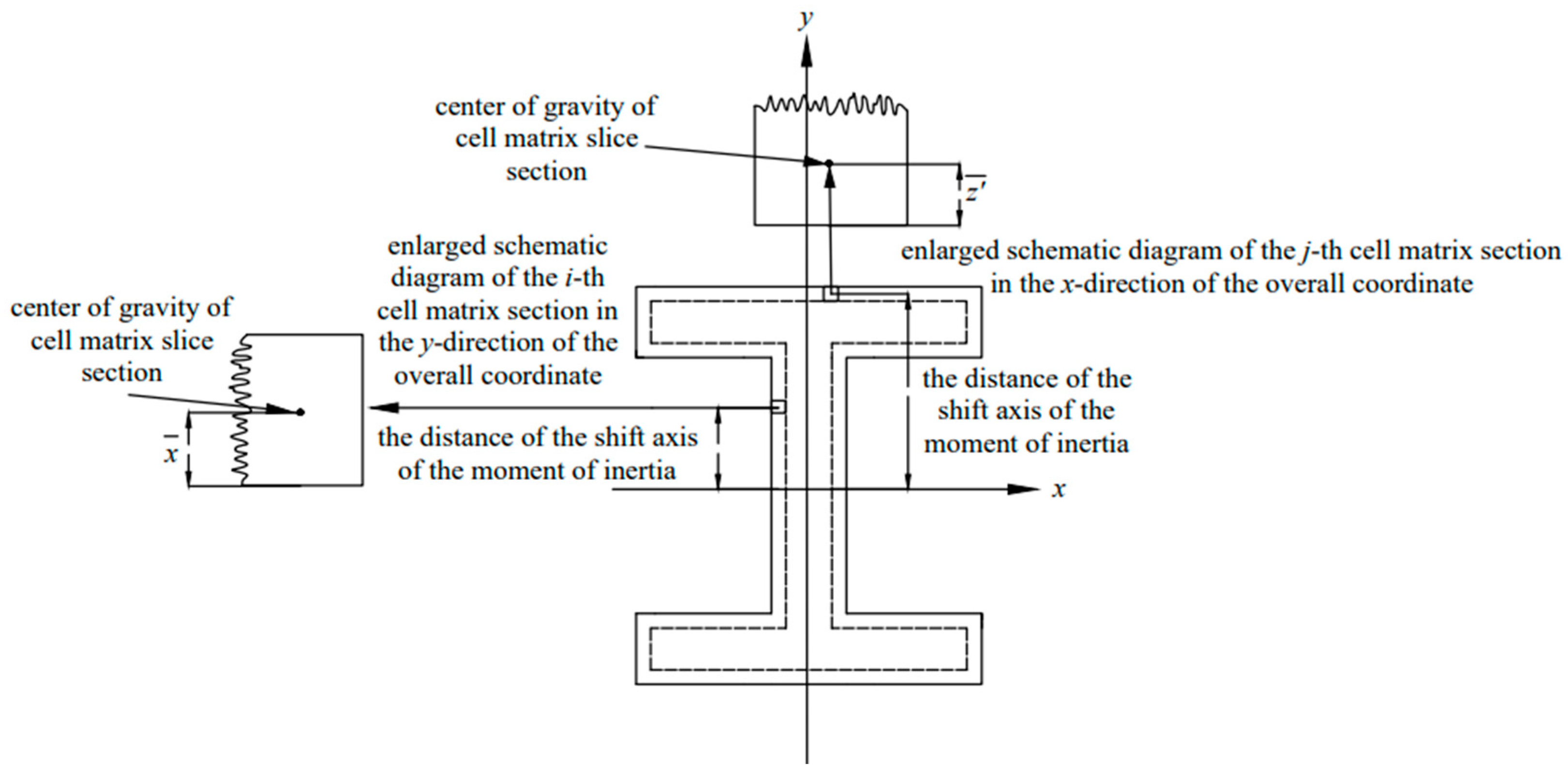
4.1. Calculation Method of Section Properties Based on Cell Matrix Slice Data

Equation (4) was used to calculate the atmospheric corrosion depth d (x_i, y_i) corresponding to coordinates (x_i, y_i).

In the x-direction of the cell matrix, slices were created according to the side length of the initial cell unit such that each slice corresponded to the coordinates of the cell matrix. The z-direction of the cell matrix was rotated by 180 degrees to obtain a new coordinate axis, and the coordinates of the new direction of the cell units were calculated:

$$k^{\prime }=L-k,$$

(10)

where k represents the original z-direction coordinate of the cell unit, k’ represents its z’-direction coordinate, and L represents the side length of the cell matrix after removing the boundary element. In this study, L = 1 mm. The coordinate transformation of the slice is illustrated in Figure 6.

The total area A of the unpassivation and passivation metal state cells of the slice cross section was:

$$A=MW{l}^2,$$

(11)

where M represents the number of unpassivation and passivation metal state cell units in the x-direction, W represents the number of unpassivation and passivation metal state cell units in the x-direction, and l represents the side length of the cell unit.

The net moment in the z’ direction was calculated for each section according to the new coordinate values:

$$S_{z^{\prime }}(i)={\displaystyle \sum _{j=1}^M{\displaystyle \sum _{k^{\prime }=1}^W\left[k^{\prime }|c(M_1,M_2)\right]}} l^2,$$

(12)

where A represents the total area of the unpassivation state metal cell unit and the passivation state metal cell unit of the slice section; S_z’ (i) represents the net moment in the z’ direction of the i-th slice section in the y direction; k’|c (M₁, M₂) represents the coordinates of the z’ direction of the unpassivation metal state cell unit M₁ and the passivation metal state cell unit M₂; j and k’ represent the j-th cell unit in the x-direction and the k’-th cell unit in the z’-direction, respectively.

The coordinate value of the centroid of the slice section in the z’-direction was then calculated:

$$\overline{z^{\prime }}=\frac{S_{z^{\prime }}(i)}{A}=\frac{S_{z^{\prime }}(i)}{MW{l}^2},$$

(13)

where A represents the total area of the unpassivation state metal cell unit and the passivation state metal cell unit of the slice section.

As shown in Figure 7, the centroid of the slice section of the cell matrix in the transformed local coordinate system was calculated. The moment of inertia of the slice section with z = z’ as the axis was calculated using Equation (14):

$$I_z(i)={{\displaystyle \sum _{j=1}^M{\displaystyle \sum _{k^{\prime }=1}^W\left[(k^{\prime }-\overline{z^{\prime }})|c(M_1,M_2)\right]}}}^2{l}^2{I}_z(i).$$

(14)

Using the same method, the net moment in the x-direction was calculated for each section:

$$S_x(i)={\displaystyle \sum _{j=1}^M{\displaystyle \sum _{k^{\prime }=1}^W\left[j|c(M_1,M_2)\right]l^2}},$$

(15)

where S_x (i) represents the net moment in the x-direction of the i-th slice section in the y-direction, and j’|c (M₁, M₂) represents the x-direction coordinate of the unpassivation metal state cell unit or the passivation metal state cell unit.

Then the coordinate value in the x-direction of the centroid of the slice section was calculated:

$$\overline{x}=\frac{S_x(i)}{A}=\frac{S_x(i)}{MW{l}^2}.$$

(16)

The moment of inertia of the slice section with $x=\overline{x}$ as the axis was calculated using Equation (17):

$$I_x(i)={\displaystyle \sum _{j=1}^M{\displaystyle \sum _{k^{\prime }=1}^W{\left[(j-\overline{x})|c(M_1,M_2)\right]}^2{l}^2}}.$$

(17)

In the structural analysis and calculation of the properties of the section of the structural steel, the cell matrix section with the smallest area was selected as the weakest section, and it was assumed that it was periodically attached to the surface of the structural steel. Taking the H-beam as an example, the calculation steps are detailed as follows.

For H-beams, we assumed that the weakest cell matrix slice section was periodically attached to all surfaces in direct contact with air, as illustrated in Figure 8. The thickness of the simulated cell corrosion layer was the side length L of the cell matrix slice section after removing boundary cell units. The area and moment of inertia of the non-cellular simulated corrosion part of the H-beam are expressed as follows:

$$A^{\prime }=2(t_{\mathrm{f}}-2L)(b-2L)+(h-2t_{\mathrm{f}}+2L)(t_{\mathrm{w}}-2L),$$

(18)

$$I_{\mathrm{x}}^{\prime }=\frac{(t_{\mathrm{w}}-2L){(h-2t_{\mathrm{f}}+2L)}^3}{12}+2(b-2L)(t_{\mathrm{f}}-2L){\left(\frac{h-t_{\mathrm{f}}}{2}\right)}^2.$$

(19)

The axis-shift theorem was applied to each cell matrix section, and the moments of inertia obtained after shifting each cell matrix section were summed to obtain the total moment of inertia in the corrosion simulation area. The areas of all cell matrix slices were also summed to obtain the total area. The corresponding schematic is shown in Figure 9, where the local coordinates refer to the coordinates of the cell matrix slice in Figure 7, and the overall coordinates refer to the coordinates of the H-beam.

The area A_c and cross-section inertia I_xc of the CA simulated corrosion were then calculated as follows:

$$\begin{array}{ll}\hfill A_{\mathrm{c}}& =2\frac{h}{L}{A}_{\mathrm{m}}+2\frac{(b-2L)}{L}{A}_{\mathrm{m}}+4\left(\frac{b-t_{\mathrm{w}}-2L}{2L}\right)A_{\mathrm{m}}\hfill \\ & =\frac{2h{A}_{\mathrm{m}}+(4b-8L-2t_{\mathrm{w}})A_{\mathrm{m}}}{L}\hfill \end{array},$$

(20)

$$\begin{array}{l}{I}_{\mathrm{xc}}={\displaystyle \sum _{i=1}^{\lfloor (h-2L)/2L\rfloor }\left\{4\left[I_{\mathrm{x}}+A_{\mathrm{m}}{\left({\overline{x}}_i\right)}^2\right]\right\}+\left(\frac{b}{L}\right)\left[I{z}^{\prime }+A\mathrm{m}{\left(\overline{z^{\prime }}+\frac{h}{2}-L\right)}^2\right]}\\ +\left(\frac{b-t_{\mathrm{w}}+2L}{L}\right)\left[I_{{\mathrm{z}}^{\prime }}+A_{\mathrm{m}}{\left(L-\overline{z^{\prime }}+\frac{h}{2}-t_{\mathrm{f}}\right)}^2\right]\end{array},$$

(21)

where A_m is the sum of the area of the unpassivation metal units and the passivation metal units in the cell matrix section with the smallest area $\overline{z^{\prime }}$ is the centroid of the z’-direction under the local coordinates of the section, $\overline{x}$ is the centroid of the x-direction under the local coordinates of the section, 2(h − 2L)/L is the number of cellmatrix slices in the y-direction in the global coordinates, and b/L + (b − t_w + 2L)/L is the number of cell matrix slices in the x-direction in the global coordinates. The minimum cross-sectional area A and inertia moment I_x of H-beam under atmospheric corrosion were calculated as follows:

$$A=A^{\prime }+A_{\mathrm{c}},$$

(22)

$$I=I_{\mathrm{x}}^{\prime }+I_{\mathrm{xc}}.$$

(23)

The minimum section resistance moment W_x in the x direction was calculated as follows:

$$W_{\mathrm{x}}=\frac{2I_{\mathrm{x}}}{h-2\left(L-d_{\mathrm{m}}\right)},$$

(24)

where d_m is the minimum corrosion depth of the cell matrix section. In the same way, parameters such as the minimum section inertia moment I_y and the minimum section resistance moment W_y in the y direction were calculated.

4.2. Analysis of Examples

An H-beam with a nominal yield strength of 235 MPa was used to analyze the effect of corrosion on section properties under the atmospheric environment of Guangzhou. The cross-sectional property, minimum cross-sectional area, and inertia moment were calculated using the proposed method. The results were compared with those obtained under the assumption of uniform corrosion.

The values of the sections without corrosion were as follows: h = 100 mm, b = 100 mm, t_w = 6 mm, and t_f = 8 mm. The average corrosion depth D (mm) under the assumption of uniform corrosion in Guangzhou was calculated using Equation (25):

$$D=0.056t^{0.41}.$$

(25)

The H-beam section properties under the assumption of uniform corrosion were calculated using the following equations [36]:

$$A^t=A^0[1-\frac{4b-2t_{\mathrm{w}}+2h}{A^0}D(t)],$$

(26)

$$I^t=I^0[1-\frac{6b{h}^2+2h^3+6(b-t_{\mathrm{f}}){(h-2t_{\mathrm{w}})}^2}{12I^0}D(t)],$$

(27)

where A^t and I^t represent the area and moment of inertia of the H-beam section in the t-th year of corrosion, respectively, and D(t) refers to the average corrosion depth in the t-th year.

The area of the smallest area and the corresponding moment of inertia calculated by the proposed method and the uniform corrosion assumption method are illustrated in Figure 10.

The minimum area and minimum moment of inertia of the section calculated by the proposed method were smaller than those of the uniform corrosion assumption.

5. Conclusions

This paper presents a method for predicting the atmospheric corrosion behavior of structural steel using three-dimensional cellular automata and a genetic algorithm. The method could simulate the surface topography of steel in different atmospheric corrosion environments.

The following are the major conclusions drawn from the results.

(1)

The proposed method could simulate the surface atmospheric corrosion of steel under different atmospheric environments, and the published experimental results have demonstrated its effectiveness. This should be useful in structural safety evaluation and performance-based design.

(2)

The accuracy of the proposed method could be improved by the cell fission mechanism. The simulation results of the Guangzhou atmospheric environment show that compared with the traditional CA method, the proposed method could reduce the maximum error from 19.3% to 1%.

(3)

The calculation method of the structure components’ cross-section inertia with non-uniform corrosion was proposed. The calculation results of the Guangzhou atmospheric environment show that the assumption of uniform corrosion will cause the structure to be unsafe.

(4)

With the accurate corrosion probability (P_c), passivation probability (P_p), passivation film rupture probability (P_b), and no-event probability (P_n), the proposed method can simulate the atmospheric corrosion of other high-performance steel structures with different strengths, materials, and properties.

In order to verify the effectiveness and expand the applied range of the proposed method, more structural steel corrosion data from different environments and of different materials should be collected, and the corrosion mechanism of different structural steels should be analyzed.

References

1. Xia, M.; Xu, S.; Wang, Y.; Li, H.; Zhao, B. Experimental study on bearing capacity of corroded Q345 H-shaped steel column under axial compression load. J. Build. Eng. 2022, 52, 104354. [Google Scholar] [CrossRef]
2. Luo, L.; Fu, H.; Zhang, Y.; Xie, X. Experimental study on the overall stability of corroded H-Shaped steel beams. Buildings 2022, 12, 1923. [Google Scholar] [CrossRef]
3. Zhang, Z.; Xu, S.; Nie, B.; Li, R.; Xing, Z. Experimental and numerical investigation of corroded steel columns subjected to in-plane compression and bending. Thin-Walled Struct. 2020, 151, 106735. [Google Scholar] [CrossRef]
4. Sharifi, Y. Uniform corrosion wastage effects on the load-carrying capacity of damaged steel beams. Adv. Steel Constr. 2012, 8, 153–167. [Google Scholar]
5. Sheng, J.; Xia, J.W.; Chang, H.F. Bending behavior of corroded H-shaped steel beam in underground environment. Appl. Sci. 2021, 11, 938. [Google Scholar] [CrossRef]
6. Wang, H.; Zhang, Z.; Qian, H.; Song, G.; Wang, J.; Fan, F. On the axial bearing capability of construction steel tube considering the uniform corrosion effect. Indian J. Eng. Mater. Sci. 2020, 27, 168–178. [Google Scholar]
7. Xu, S.H.; Ren, S.B.; Wang, Y.D. Three-dimensional surface parameters and multi-fractal spectrum of corroded steel. PLoS ONE 2015, 10, 0131361. [Google Scholar] [CrossRef] [Green Version]
8. Zhao, Z.; Mo, S.; Xiong, Q.; Liu, H.; Liang, B. Moment capacity of H-section steel beam with randomly located pitting corrosion. Probabilistic Eng. Mech. 2021, 66, 103161. [Google Scholar] [CrossRef]
9. Wu, B.; Cao, J.L.; Kang, L. Influence of local corrosion on behavior of steel I-beams subjected to end patch loading: Experiments. J. Constr. Steel Res. 2017, 135, 150–161. [Google Scholar] [CrossRef]
10. Kim, I.-T.; Lee, M.-J.; Ahn, J.-H.; Kainuma, S. Experimental evaluation of shear buckling behaviors and strength of locally corroded web. J. Constr. Steel Res. 2013, 83, 75–89. [Google Scholar] [CrossRef]
11. Ahn, J.-H.; Cheung, J.-H.; Lee, W.-H.; Oh, H.; Kim, I.-T. Shear buckling experiments of web panel with pitting and through-thickness corrosion damage. J. Constr. Steel Res. 2013, 115, 290–302. [Google Scholar] [CrossRef]
12. Khurram, N.; Sasaki, E.; Katsuchi, H.; Yamada, H. Experimental and numerical evaluation of bearing capacity of steel plate girder affected by end panel corrosion. Int. J. Steel Struct. 2015, 14, 659–676. [Google Scholar] [CrossRef]
13. Cao, J.L. Research on the End Partial Compression Performance and Reinforcement of Locally Corroded H-Beams; South China University of Technology: Guangzhou, China, 2019. [Google Scholar]
14. Wang, R.H.; Fang, Y.Y.; Dou, P.L.; Sun, J. Research on the ultimate bearing capacity of leg column axial compression of pile-based platform under pitting damage. Ocean Eng. 2015, 33, 1–7. [Google Scholar]
15. Wang, H.; Yu, Y.; Yu, J.; Duan, J.; Zhang, Y.; Li, Z.; Wang, C. Effect of 3D random pitting defects on the collapse pressure of pipe—Part I: Experiment. Thin-Walled Struct. 2018, 129, 512–526. [Google Scholar] [CrossRef]
16. Wang, H.; Yu, Y.; Yu, J.; Jin, C.; Zhao, Y.; Fan, Z.; Zhang, Y. Effect of 3D random pitting defects on the collapse pressure of pipe—Part II: Numerical analysis. Thin-Walled Struct. 2018, 129, 527–541. [Google Scholar] [CrossRef]
17. Wang, R.H.; Tong, Z.J.; Guo, H.C. Research on the influence of random distribution pitting corrosion on the ultimate strength of circular steel pipe section. Ocean Eng. 2018, 36, 1–8. [Google Scholar] [CrossRef]
18. Wang, R.H.; Ajit, S.R.; Adam, S. Ultimate strength assessment of plated steel structures with random pitting corrosion damage. J. Constr. Steel Res. 2018, 143, 331–342. [Google Scholar] [CrossRef] [Green Version]
19. Liu, Y.E.; Lin, C.; Zhao, Q. Corrosion behavior of carbon steel in SO2 atmosphere. Chin. J. Corros. Prot. 2010, 30, 51–57. [Google Scholar] [CrossRef]
20. Zhang, L.; Wang, Z.Y.; Zhao, C.Y.; Cao, G.W.; Liu, Y.J. Corrosion behavior of carbon steel and weathering steel in salt spray environment. Equip. Environ. Eng. 2014, 43, 1–6. [Google Scholar]
21. Chen, W.; Hao, L.; Dong, J.; Ke, W.; Wen, H. Effect of pH value on the corrosion evolution of Q235B steel in simulated coastal-industrial atmospheres. Acta Metall. Sin. 2015, 52, 191–200. [Google Scholar] [CrossRef]
22. Guo, X.M.; Pan, C.; Wang, Z.Y.; Han, W. Research on initial corrosion behavior of carbon steel in simulated marine industrial atmospheric environment. Acta Metall. Sin. 2015, 54, 65–75. [Google Scholar] [CrossRef]
23. Guo, J.K.; Yu, J.S.; Peng, X.; Yin, L.; Cao, S.A. Study on the atmospheric corrosion behavior of carbon steel using accelerated corrosion test. Surf. Technol. 2014, 43, 68–73. [Google Scholar] [CrossRef]
24. Dong, J.H.; Ke, W. The accelerated test of simulated atmospheric corrosion and the rust evolution of low carbon steel. J. Electrochem. 2009, 15, 170–178. [Google Scholar] [CrossRef]
25. Gao, C.; Zheng, S.S.; Hu, W.B.; Zhang, X.H.; Liu, Y. Review of research on mechanical properties of steel structure under atmospheric environment corrosion. Mater. Rep. 2020, 34, 11162–11170. [Google Scholar] [CrossRef]
26. Pérez-Brokate, C.F.; di Caprio, D.; Féron, D.; De Lamare, J.; Chaussé, A. Overview of cellular automaton models for corrosion. In Proceedings of the 11th International Conference on Cellular Automata for Research and Industry (ACRI), Krakow, Poland, 22–25 September 2014. [Google Scholar] [CrossRef]
27. Jahns, K.; Balinski, K.; Landwehr, M.; Wübbelmann, J.; Krupp, U. Prediction of high temperature corrosion phenomena by the cellular automata approach. Mater. Corros.-Werkst. Und Corros. 2017, 68, 125–132. [Google Scholar] [CrossRef]
28. Lishchuk, S.; Akid, R.; Worden, K.; Michalski, J. A cellular automaton model for predicting intergranular corrosion. Corros. Sci. 2011, 53, 2518–2526. [Google Scholar] [CrossRef]
29. Wang, H.; Lv, G.Z.; Wang, L.; Zhang, Y.H. Cellular automaton simulations of surface corrosion damage evolution. Acta Aeronaut. Astronaut. Sin. 2008, 29, 1490–1496. [Google Scholar]
30. Hua, L.; Liu, X.F.; Chang, D.M. Study on multi-pits corrosion of aluminum alloy and its fatigue life based on cellular automata. Areonautical Sci. Technol. 2021, 32, 63–67. [Google Scholar] [CrossRef]
31. Stafiej, J.; Caprio, D.D.; Bartosik, Ł. Corrosion-passivation processes in a cellular automata based simulation study. J. Supercomput. 2013, 65, 697–709. [Google Scholar] [CrossRef] [Green Version]
32. Cui, C.; Ma, R.; Chen, A.; Pan, Z.; Tian, H. Experimental study and 3D cellular automata simulation of corrosion pits on Q345 steel surface under salt-spray environment. Corros. Sci. 2019, 154, 80–89. [Google Scholar] [CrossRef]
33. Guo, D.X.; Ren, K.L.; Wang, Y.C.; Guo, X.J.; Zhang, E.S. Three-dimensional cellular automata model for predicting local corrosion. Mech. Eng. 2014, 36, 447–452. [Google Scholar]
34. Gu, X.Y.; Kang, J.F.; Zhu, J.S. 3D cellular automata-based numerical simulation of atmospheric corrosion process on weathering steel. J. Mater. Civ. Eng. 2018, 30, 04018296. [Google Scholar] [CrossRef]
35. Yao, J.T.; Zhao, G.F.; Pu, Y.X. Probabilistic models for resistance of structures in design and in service. Build. Sci. 2005, 21, 13–15. [Google Scholar] [CrossRef]
36. Luo, L.S.; Chen, Z.H.; Zhao, X.L.; Zhang, Y. Deterioration model for resistance of steel member in atmospheric environment. Struct. Eng. 2019, 35, 52–58. [Google Scholar] [CrossRef]
37. Xu, S.H.; Nie, B.; Zhang, H.J. Time-dependent reliability analysis for corroded RC beams based on probability density evolution theory. J. Build. Struct. 2020, 47, 75–83. [Google Scholar] [CrossRef]
38. Seghier, M.E.B.; Hoche, D.; Zheludkevich, M. Prediction of the internal corrosion rate for oil and gas pipeline: Implementation of ensemble learning techniques. J. Nat. Gas Sci. Eng. 2022, 99, 104425. [Google Scholar] [CrossRef]
39. Seghier, M.E.A.B.; Corriea, J.A.F.O.; Jafari-Asl, J.; Malekjafarian, A.; Plevris, V.; Trung, N.-T. On the modeling of the annual corrosion rate in main cables of suspension bridges using combined soft computing model and a novel nature-inspired algorithm. Neural Comput. Appl. 2021, 33, 15969–15985. [Google Scholar] [CrossRef]
40. Liang, C.F.; Hou, W.T. Sixteen-year atmospheric corrosion exposure study of steels. J. Chin. Soc. Corros. Prot. 2015, 25, 1–6. [Google Scholar]
41. Xiao, S.Y. Research on Surface Characteristics and Stochastic Constitutive Model of Corroded Steel in General Atmosphere and Offshore Atmosphere; Xi’an University of Architecture and Technology: Xi’an, China, 2020. [Google Scholar]
42. Tan, T.D.; Chen, Y.T.; Chen, H.J. An improved mesoscopic oxidation model of metals in lead bismuth eutectic. Comput. Mater. Sci. 2008, 43, 251–267. [Google Scholar] [CrossRef]
43. Weeeen, P.C.D.; Zimer, A.; Pereira, E. Modeling pitting corrosion by means of a 3D discrete stochastic mode. Corros. Sci. 2014, 82, 133–144. [Google Scholar] [CrossRef]
44. Zhang, B.; Wang, X.; Dong, C.; Ji, H. Comparison of corrosion models of bridge structural steel in Qingdao marine atmosphere. J. Highw. Transp. Res. Dev. 2013, 301, 69–73. [Google Scholar] [CrossRef]
45. Bhandari, J.; Khan, F.; Abbassi, R.; Garaniya, V.; Ojeda, R.; Rabanal, R.O. Pitting degradation modeling of ocean steel structures using Bayesian Network. J. Offshore Mech. Arct. Eng. 2017, 5, 051402. [Google Scholar] [CrossRef]
Figure 1. Publish test comparison results of corroded and uncorroded beams. (a) corroded beam; (b) load-deformation curves comparison results of different specimens [1].
Buildings 13 00253 g001
Figure 2. Cellular Automata (CA) calculation rules. (a) a Moore neighborhood rules of CA; (b) a periodic boundary of CA.
Buildings 13 00253 g002
Figure 3. CA-GA algorithm block diagram for atmospheric corrosion simulation.
Buildings 13 00253 g003
Figure 4. A steel’s surface atmospheric corrosion simulation results at different times. (a) steel corrosion simulation results in 1 year; (b) steel corrosion simulation results in 4 years; (c) steel corrosion simulation results in 8 years; (d) steel corrosion simulation results in 16 years.
Buildings 13 00253 g004
Figure 5. Comprehensive errors comparison of simulation results with and without cellular fission mechanism.
Buildings 13 00253 g005
Figure 6. Schematic diagram of the coordinate transformation of slices.
Buildings 13 00253 g006
Figure 7. Schematic diagram of the cell matrix slice section.
Buildings 13 00253 g007
Figure 8. Schematic diagram of cell matrix slice section and attachment of H-beam section.
Buildings 13 00253 g008
Figure 9. Schematic diagram of the axis-shifting process of the inertia moment of the H-beam cell matrix section.
Buildings 13 00253 g009
Figure 10. Comparison of simulation results with different calculation methods. (a) simulation results of the minimum cross-sectional area; (b) a simulation result of the minimum section’s inertia moment.
Buildings 13 00253 g010