Article

Dynamic Characterisation of a Heritage Structure with Limited Accessibility Using Ambient Vibrations

1
Department of Structural Engineering, Faculty of Engineering, Cairo University, Giza 12613, Egypt
2
Department of Archaeological Conservation, Faculty of Archaeology, Cairo University, Giza 12613, Egypt
3
School of Sustainability, Civil and Environmental Engineering, University of Surrey, Guildford GU2 7XH, UK
4
Department of Civil and Environmental Engineering, Imperial College London, London SW7 2AZ, UK
*
Authors to whom correspondence should be addressed.
Buildings 2023, 13(1), 192; https://doi.org/10.3390/buildings13010192
Submission received: 24 November 2022 / Revised: 3 January 2023 / Accepted: 5 January 2023 / Published: 11 January 2023

Abstract

:
Historic Cairo has been a UNESCO World Heritage Site since 1979. It has more than 600 historic structures, which require extensive studies to sustain their cultural, religious, and economic values. The main aim of this paper is to undertake dynamic investigation tests for the dome of Fatima Khatun, a historic mausoleum in Historic Cairo dating back to the 13th century and consisting of mainly bricks and stones. The challenge was that the structure was difficult to access, and only a small portion of the top was accessible for the attachment of accelerometers. Current dynamic identification procedures typically adopt methods in which the sensors are arranged at optimal locations and permit direct assessment of the natural frequencies, mode shapes, and damping ratios of a structure. Approaches that allow for the evaluation of dynamic response for structures with limited accessibility are lacking. To this end, in addition to in situ dynamic investigation tests, a numerical model was created based on available architectural, structural, and material documentation to obtain detailed insight into the dominant modes of vibration. The free vibration analysis of the numerical model identified the dynamic properties of the structure using reasonable assumptions on boundary conditions. System identification, which was carried out using in situ dynamic investigation tests and input from modelling, captured three experimental natural frequencies of the structure with their mode shapes and damping ratios. The approach proposed in this study informs and directs structural restoration for the mausoleum and can be used for other heritage structures located in congested historic sites.

1. Introduction

Non-destructive monitoring techniques can be adopted for assessing the structural health condition of heritage buildings and provide means to develop suitable integrated maintenance and intervention plans [1]. Assessment and conservation of such buildings are vital for the preservation of cultural identity as well as the overall improvement of historic centres [2]. Dynamic monitoring systems have been extensively used for structures with high geometric complexity or significant inhomogeneities in constituent materials [3]. Dynamic testing offers information regarding the global structural behaviour and can be adopted for the calibration of numerical models of structures [4]. These tests are typically used to provide detailed insights into the modal parameters of a structure, namely its natural frequencies, mode shapes, and damping ratios [5].
This testing technique is often preferred for cultural heritage, for which the need to maintain the historical value of the structure imposes constraints regarding the range of appropriate approaches for system characterisation [6]. Such tests involve measuring, typically using accelerometers, the structural movements under a free vibration or external excitation [7]. By conducting signal processing on the captured vibrations, the in situ dynamic properties of the structure can be determined. Two test methods are commonly used for the purpose of dynamic investigation, namely forced vibration testing (FVT) and ambient vibration testing (AVT), although other non-contact methods using remote devices such as interferometric radars have also been used [8,9]. These methods were employed for a wide range of heritage structures such as bell towers, arched structures or domes, and other monumental structures [9,10,11,12,13]. FVT and AVT dynamic methods can also be used in conjunction with digital image processing, infrared thermography, laser levelling, and ground-penetrating radar [14], as well as refined finite element or analytical models [15,16].
In the FVT method, the structure is excited through an external force such as a mechanical shaker at a specific location. The response is measured at locations other than the excitation points to identify the structural properties through frequency response functions (FRF’s) in matrix form representing the change in the input signal due to the structural response. Every structure has its unique FRF, which may be used to determine the modal parameters [17]. Bartoli et al. [18] used FVT during their dynamic investigation of the Italian Medieval “Torre Grossa” of San Gimignano. They used an actuator for forced excitations twice: once for the excitation in the x-direction and another for that in the y-direction. Ramos et al. [12] evaluated the damage in arched masonry structures through combined dynamic damage identification methods, indicating the suitability of various dynamic processing methods for crack detection.
FVT can be disruptive and expensive, whilst ambient vibration tests (AVT) offer a non-disruptive alternative to measure the structural vibrations caused by operational conditions such as wind, neighbouring activities, traffic flow, and micro-tremors as operational conditions [2,19]. An AVT excitation is typically stochastic noise or white noise; therefore, only output measurements can be used to identify modal parameters, typically referred to as “output-only measurements” [20]. Assessment of the modal parameters from ambient vibration data is typically performed by using the Frequency Domain Decomposition (FDD) technique in the frequency domain and the data-driven Stochastic Subspace Identification (SSI) method, but other methods can also be adopted [13].
The AVT method is commonly used for heritage structures as it requires no excitations, although it involves significantly more post-processing effort than FVT for estimating the uncertain structural parameters [20,21]. Non-destructive tests using ambient vibrations have been employed for dynamic structural identification of multi-leaf masonry walls that have intrinsic structural complexity, heterogeneity, and irregularity [22]. Ivorra and Pallarés [10] undertook dynamic tests on the “Nuestra Sra. De la Misericordia Church” (Valencia, Spain) bell tower structure using two piezoelectric accelerometers, placed at the height of the bell house. The dynamic testing results were used to calibrate numerical models and determine the bending and torsion frequencies of the tower and informed the bell restoration. Similar procedures were adopted to assess the post-earthquake structural response of the Gabbia Tower (Italy) and to inform seismic vulnerability assessments [11], as well as to understand the sensitivity of dynamic measurements to safety interventions [23]. AVT performed on the bell tower of the Santa Sofia in Benevento (Italy) was used in conjunction with dynamic response assessments for the subsoil at the tower to calibrate a refined numerical model [24]. It was shown the soil contributes extensively to the higher response modes corresponding to the second bending modes. Tomograph devices and microtremor assessments allowed the evaluation of the relationship between damage, frequencies, and base amplification of the Radha Krishna and Pancha Deval Temples in Nepal, indicating direct correlation between higher frequencies and higher level of damage for the structures investigated [25].
In situ dynamic investigations are typically made with accelerometers or geophones positioned at critical locations on or within the structure, hence enabling effective signal processing to estimate its dynamic properties [26]. This “System Identification” process requires different setups for cross-correlation during the signal processing of the captured vibrations. In optimal conditions, the instrumentation is positioned either inside the building [6,27,28] or at the exterior of the monument [1,29,30].
In congested sites, such as those in Historic Cairo, the limited accessibility to the main areas of the structures poses challenges in setting the instrumentation in optimal locations. This the case of Fatima Khatun mausoleum, which is assessed within this project [31,32,33]. As described in this paper, only one setup was utilised due to inaccessibility issues, which led to extracting data from a small part of the structure at just three nearby points located at the same level. The one-setup problem caused some difficulties during the signal processing step, so a new approach is proposed to overcome this problem. This approach is verified by a theoretical validation model, after which, it is utilised to successfully complete the signal processing of the collected data by extracting the dynamic properties of the structure. The proposed approach, which includes in situ dynamic tests and numerical modelling, can be used for other heritage structures located in congested historic sites.
This approach provides the ability to extract the dynamic properties of a structure with inaccessibility issues, which might lead to capturing acceleration data using only one setup with few nearby points instead of a full investigation of all the proposed setups that cover all mode shapes. Moreover, this approach utilises common methods in signal processing techniques that can be easily applied to similar structures under investigation. However, the proposed approach is limited to structures that can be excited only by ambient vibrations of the surrounding environment. Moreover, the approach has not been verified for dealing with more than 10% noise, as it has been validated using a theoretical model with added noise of 10% of the amplitude of the captured signal.
The next section introduces the heritage dome structure under investigation in this study. It provides historical information about the structure, its geometric description, and material characteristics. Section 3 focuses on the in situ tests and their analysis. It starts with an overview of the approaches used in signal processing, followed by a description of the setup used during the data acquisition step, and it finally provides an analysis using the “peak picking” method. Subsequently, Section 4 starts by describing a numerical model of the structure to understand the modal behaviour of the dome and to validate the proposed approach. After verifying the model, the proposed approach is used to analyse the experimental data in order to extract the dynamic properties of the structure and to relate it to the numerical mode shapes. This is followed by Section 5, which provides a discussion of the results obtained during the signal processing of the acquired data. The final section outlines the main conclusions of this study.

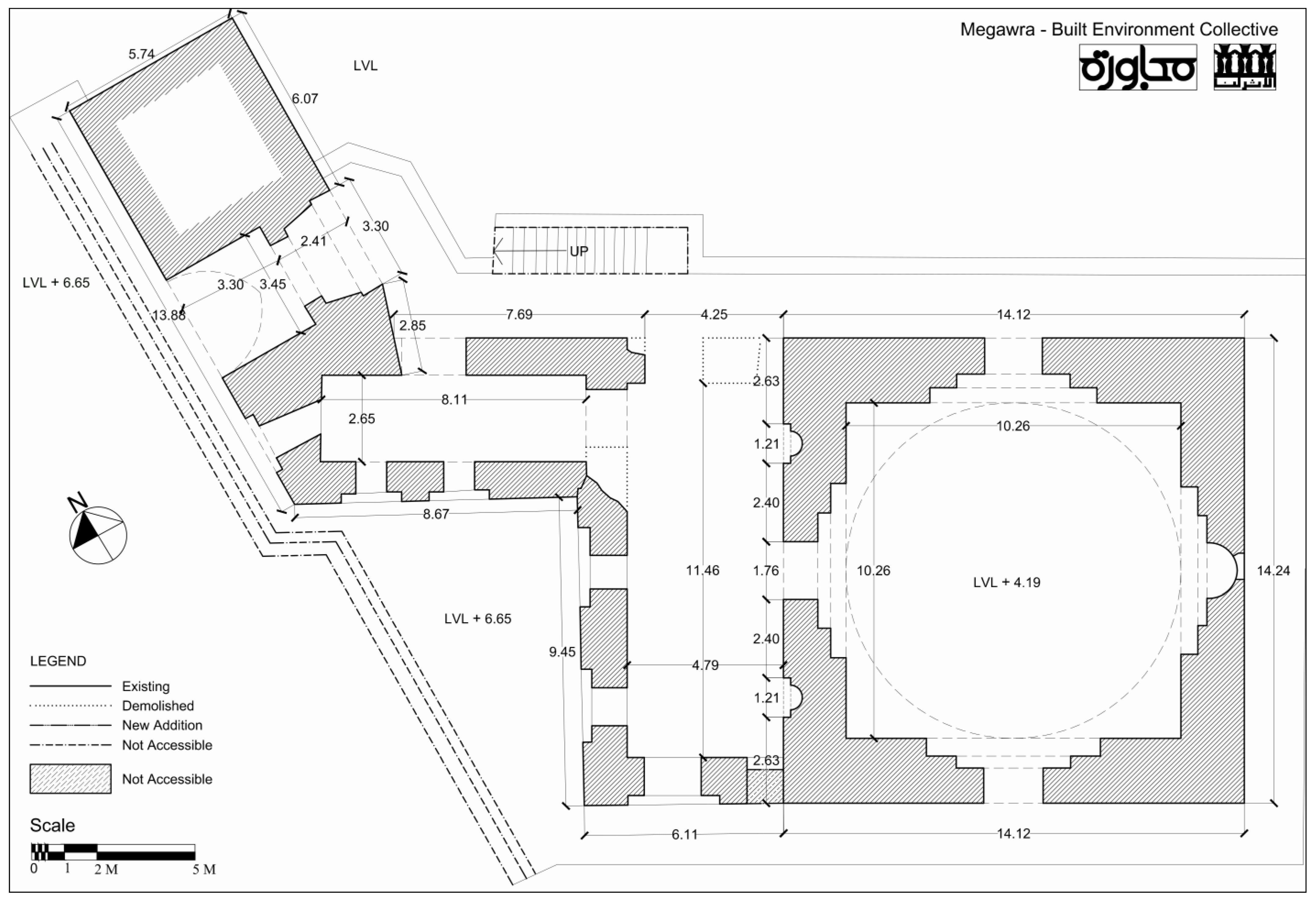
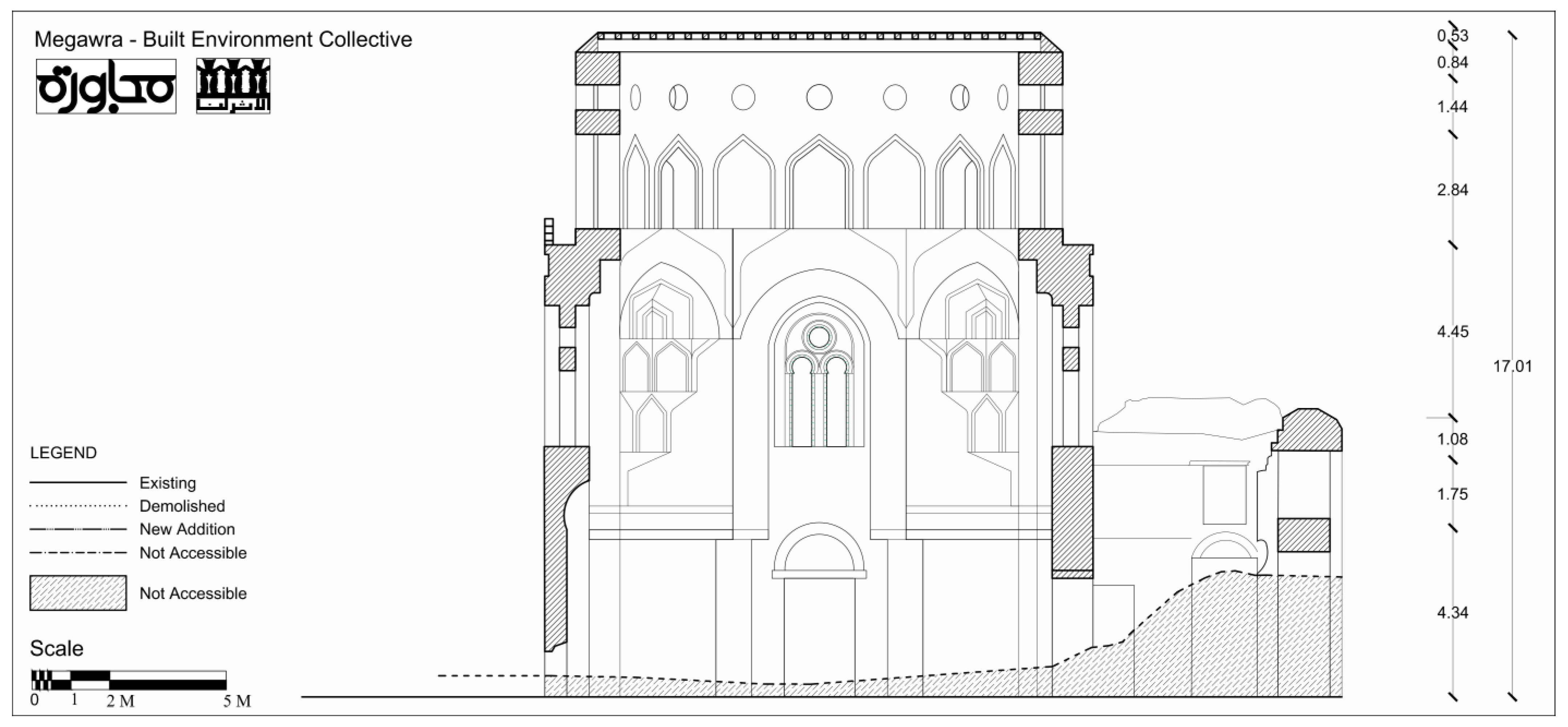
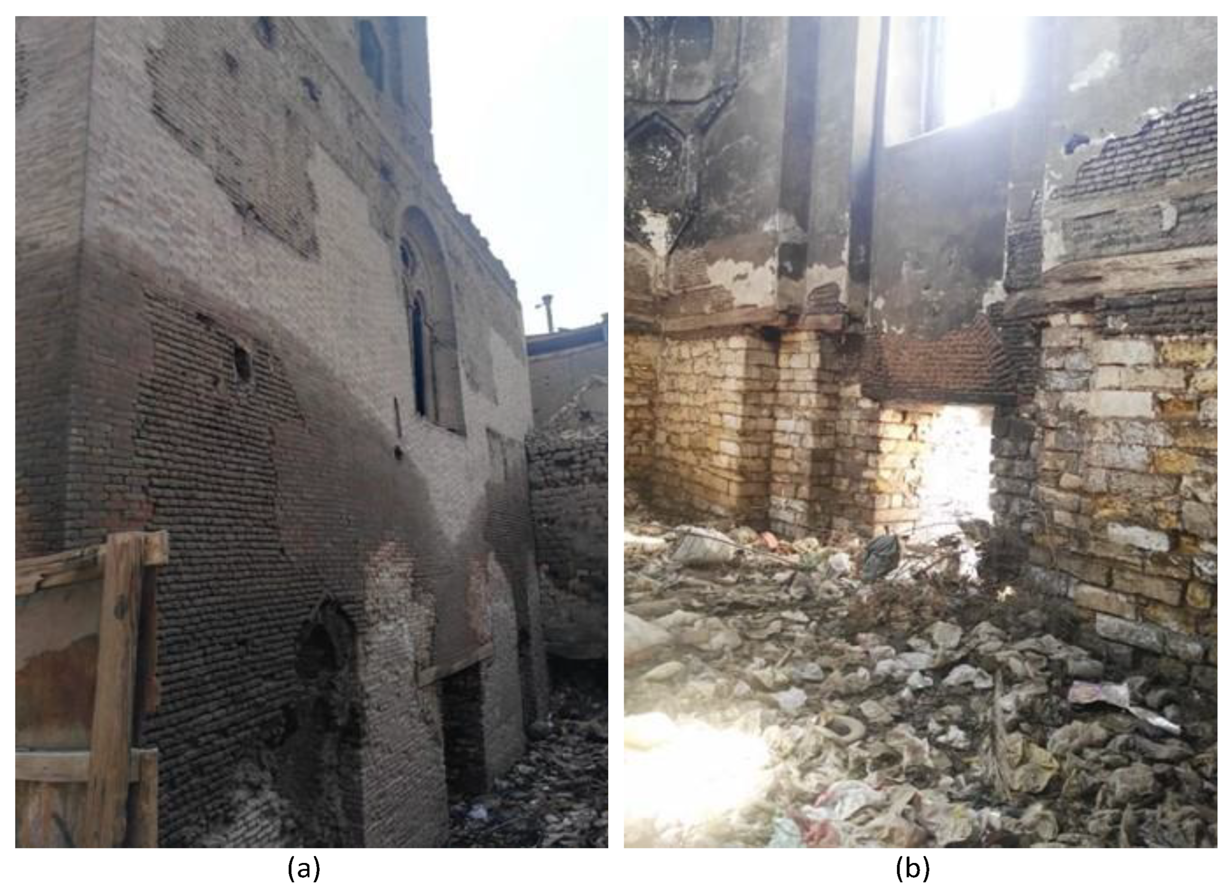
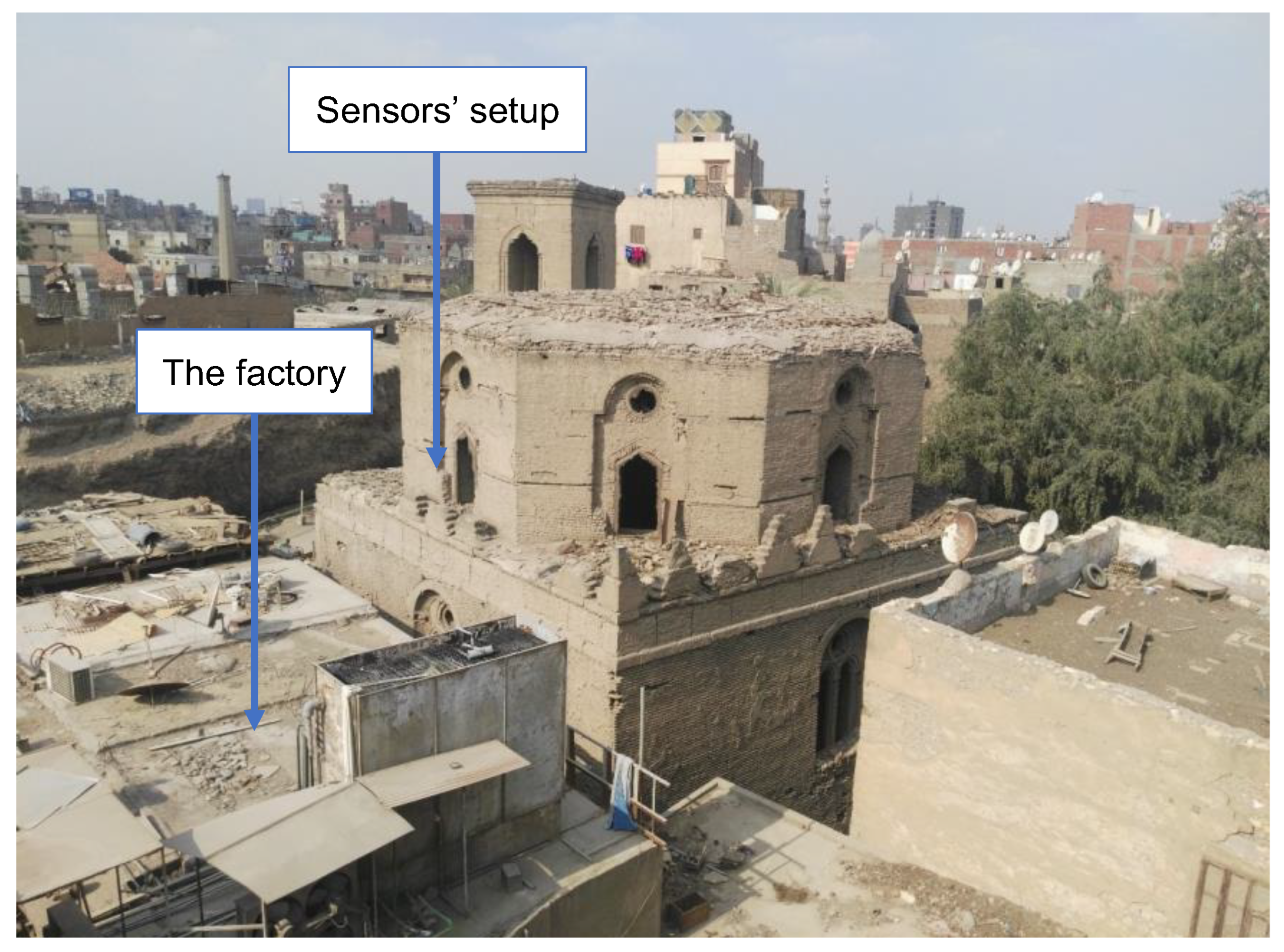
2. Structural Configuration

The Dome of Fatima Khatun is a large masonry chamber located at Al-Ashraf Street beside the Mosque of Al-Sayeda Nafisa in Cairo, as shown in Figure 1. It was built in 1284 under the order of Sultan al-Mansour Qalawun and named after his wife [34,35]. There are some deteriorated walls beside the dome from the north-west direction along with a minaret which belongs to a madrasa (school) [36]. Sonbol [37] suggests that the school construction was a request from Fatima Khatun to extend the benefits of her building. Two deteriorated walls of the school are shown in Figure 2.
The structure is investigated according to available data and visual inspection. The Megawra NGO [38] provided a recent conservation study for the structure, which was used to determine the geometry. At its foundation level, the chamber is square with an internal side length of 10.25 m from the inside up to an elevation of 11.75 m; thereafter, the perimeter is changed into an octagon with an internal side length of 4.25 m. This change is achieved through a transition zone of muqarnas (Islamic archetypal form originated from squinches). Hence, the dome consists mainly of four perpendicular walls up to a height of 11.75 m. These walls support four walls of an octagon of 4.85 m height, and the other four walls of the octagon are supported on a transition zone of squinches, leading to a total height of 16.6 m for the dome (Figure 3). The roof of the structure was originally built from a masonry dome, but this no longer exists and was later replaced by a temporary wooden roof. An elevation view of one of the façades of the dome is shown in Figure 4, in which it can be seen that the other three façades share the same geometry and are practically identical. Figure 5 also shows the plan symmetry of the geometry of the dome.
Figure 1. The location of the dome of Fatima Khatun at Al-Khalifa region (Reproduced with permission from MEGAWRA-BEC, unpublished report, 2017 [39]).
Buildings 13 00192 g001
Figure 2. (a) The dome of Fatima Khatun (looking south). (b) Remains of the deteriorated school attached to the structure (looking south-west).
Buildings 13 00192 g002
Figure 3. Elevation levels (looking north).
Buildings 13 00192 g003
Figure 4. CAD drawing of the north-west elevation of the dome of Fatima Khatun (Reproduced with permission from MEGAWRA-BEC, unpublished report, 2017 [38]).
Buildings 13 00192 g004
Figure 5. Sectional Plan of the dome of Fatima Khatun, along with the deteriorated walls of the school and the minaret (Reproduced with permission from MEGAWRA-BEC, unpublished report, 2017 [38]).
Buildings 13 00192 g005
Each of the four perpendicular walls has a thickness of about two meters except for two inside recesses in the middle. The first recess has a width of 5.3 m, with a thickness of 0.5 m and a height of 11.3 m, and the second recess has a width of 3.5 m with a thickness of 0.4 m and a height of 10.6 m. Hence, the overall wall thickness is about 1.1 m in the location of the two recesses, as shown in Figure 5. On the other hand, the octagonal walls have a uniform thickness of about 1.1 m. Each of the four perpendicular walls has a thickness of about two meters except for two inside recesses in the middle. As shown in Figure 6, the first recess has a width of 5.3 m with a thickness of 0.5 m and a height of 11.3 m, and the second recess has a width of 3.5 m with a thickness of 0.4 m and a height of 10.6 m. Hence, the overall wall thickness is about 1.1 m in the location of the two recesses. On the other hand, the octagon walls have a uniform thickness of about 1.1 m.
The dome is founded on two layers of limestone blocks, and the foundation thickness is about 0.8 m. The dome consists mainly of old solid clay bricks, along with timber members in a few locations. New solid clay bricks were found in all elevations of the dome, except at the south-east elevation, which was placed within subsequent interventions for which no information is available. Figure 7a clearly shows the difference between new and old bricks. Another intervention may have occurred from the inside to restore the walls, but it seems that this intervention was performed using small blocks of ashlar limestone, as shown in Figure 7b.

3. Dynamic Investigation Tests

3.1. Signal Processing Approaches

Fast Fourier Transform (FFT) can be used to transfer the collected data from the time domain to the frequency domain. This transformation gives the spectrum of frequencies of the recorded channel in which peaks indicate natural frequencies of the structure in most cases for the ambient vibration methods. Power spectral density (PSD) is another method to visually select peaks to manually detect natural frequencies of the structure. PSD is recommended to analyse the data of random processes, such as the measured acceleration of a structure exposed to white noise excitation due to external effects; i.e., ambient vibrations [40].
There are various approaches to estimate PSD based on the acceleration response of a structure. One of these is Welch’s method [41], which depends on using overlapped segments of the response by taking the mean of these segments [40]. This technique requires a large dataset to make the results reliable, which is typically the case for applications in structural engineering, making Welch’s method the most suitable to estimate PSD using a direct procedure. Other conventional approaches include the Periodogram method, the Modified Periodogram method, Bartlett’s method, and the Blackman–Tukey method [42].
Welch’s method employs windowing during the estimation of the PSD, which reduces spectral leakage caused by the non-integer number of periods of the signal while transforming from the time domain to the frequency domain using Fast Fourier Transform (FFT). Applying a window involves multiplying the segment of the signal by an amplitude that varies gradually from zero to generate periodic signals instead of sharp-edged signals, which cause spectral leakage. There are many window functions that result in this smooth transition of the signals, including the Hamming window, which is the default with the pwelch command in MATLAB [43]. Choosing the window function depends on the application in which the PSD is used and the type of the signals. For example, if the data contain narrowband random signals, Hamming window is used; whereas if the amplitude of the PSD is important, a Flat Top window is used. Other window functions include Kaiser–Bessel, Uniform, Exponential, and Force window [44].
The mode shapes of the structure can be calculated at selected frequencies using different methods. The most basic of which is using the FFT to compare the amplitudes of all channels along with the phase angle of each channel at the same frequency to estimate the mode shape relative to one channel. This method is straightforward, but it encounters some problems if the signal is noisy. Another approach is using the Frequency Domain Decomposition (FDD) technique to calculate the mode shape using the acceleration response after transforming the data into the frequency domain. Alternatively, Time Domain Decomposition (TDD) can be adopted, which is a similar method to the FDD technique but calculates the mode shape in the time domain with the ability to give an estimate for the damping ratio at each selected frequency. Farshchin [45] presented an open-source MATLAB code to determine mode shapes based on the FDD technique for output-only data, which is the case for structures excited by ambient vibrations. Cheynet [46] enhanced this code to develop an automated tool based on the FDD technique, referred to as AFDD, with the ability to estimate the damping ratios of each mode. Another open-source MATLAB code was also developed by Cheynet [47] to determine mode shapes based on the TDD technique for the same type of data. Other commercial software for operational and experimental modal analysis is available for signal processing of the collected data using different techniques in the frequency domain or in time domain such as ARTeMIS Modal [48], as well as MACEC [49], which is a MATLAB toolbox designed for this purpose.

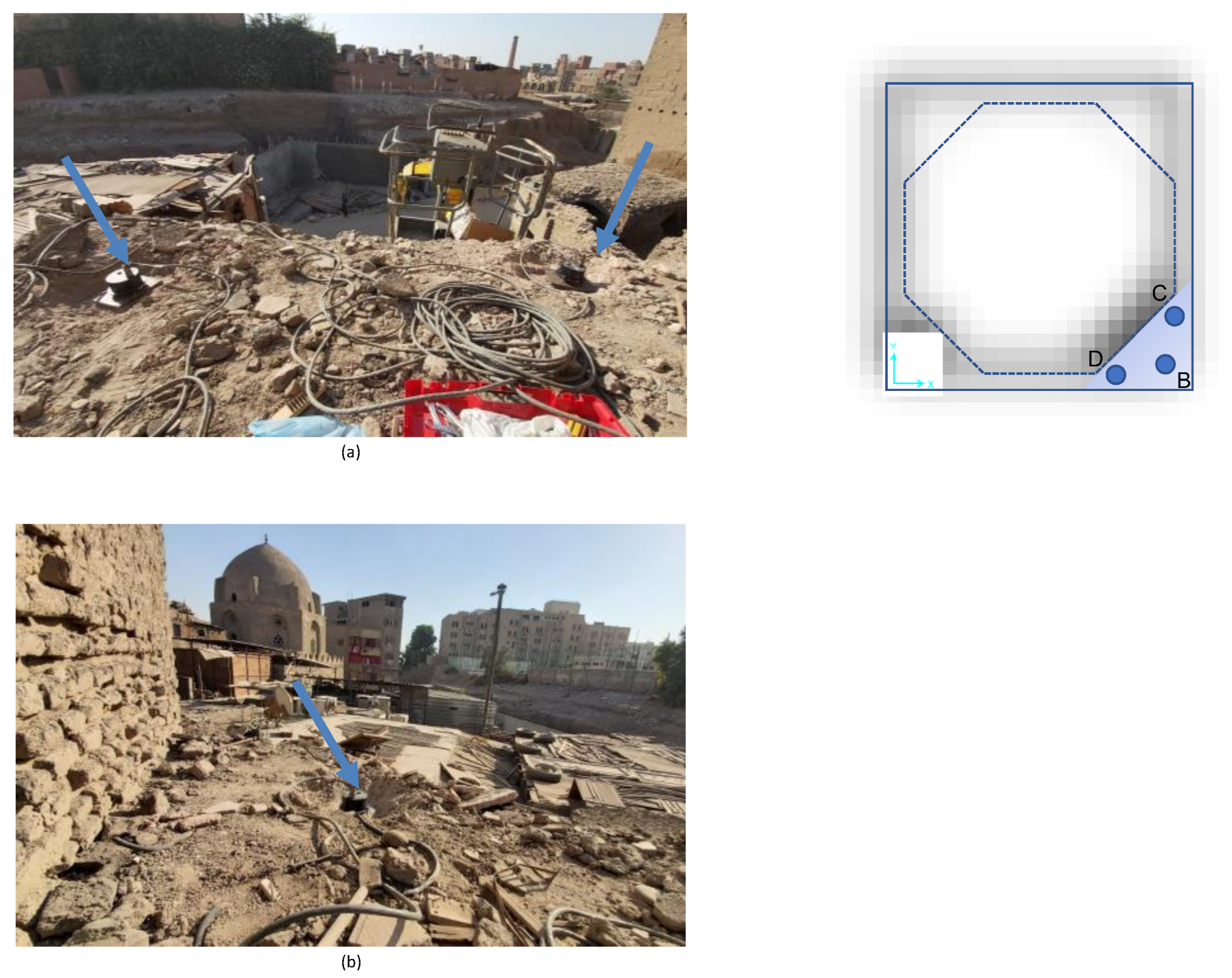
3.2. Testing Arrangements

Ideally, sensors should be placed at the two main levels of the structure (Figure 3) and distributed in plan. However, due to accessibility issues, the installed setup was limited to the only reachable area, which is the shaded part in panel at the top right-hand side of Figure 8. Only three Kinemetric triaxial sensors [50] with a sampling frequency of 100 Hz were installed near the edges. Figure 8 shows the full setup of the three sensors. The test setup was installed on 24 September 2019, when the temperature was 32 °C.
Three 50 m long cables connected the accelerometers to the data acquisition system, such that it could be placed on the ground. Data registration was carried out twice: Measurement One (M1) started at 3:17 p.m. for 10 min, and Measurement Two (M2) started at 3:27 p.m. for 20 min. The data were saved in two ASCII files, one for each measurement, and each file included data from nine channels. A representative example of the collected data is illustrated in Figure 9, which shows the acceleration response of Sensor “B” for M2, which represents the vibration of the structure under ambient noise conditions in three perpendicular directions. During the data acquisition, it was noted that some motors were running in an adjacent ice cream factory. Further investigation indicated that the frequencies of these motors were 30 and 50 Hz.

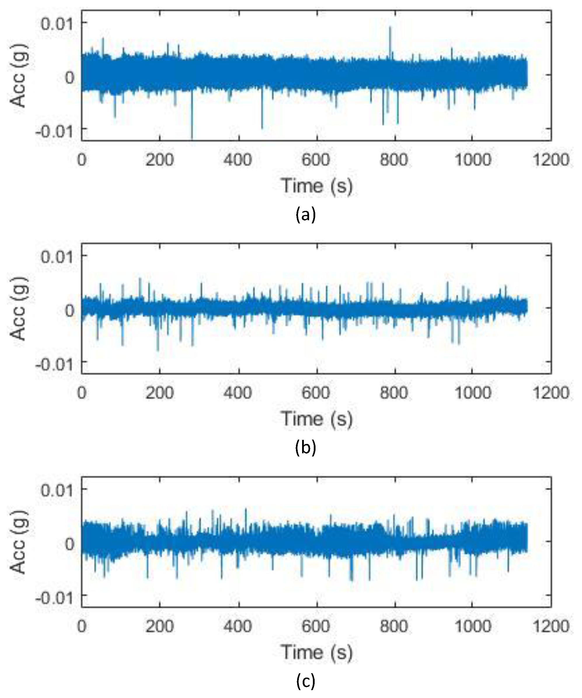
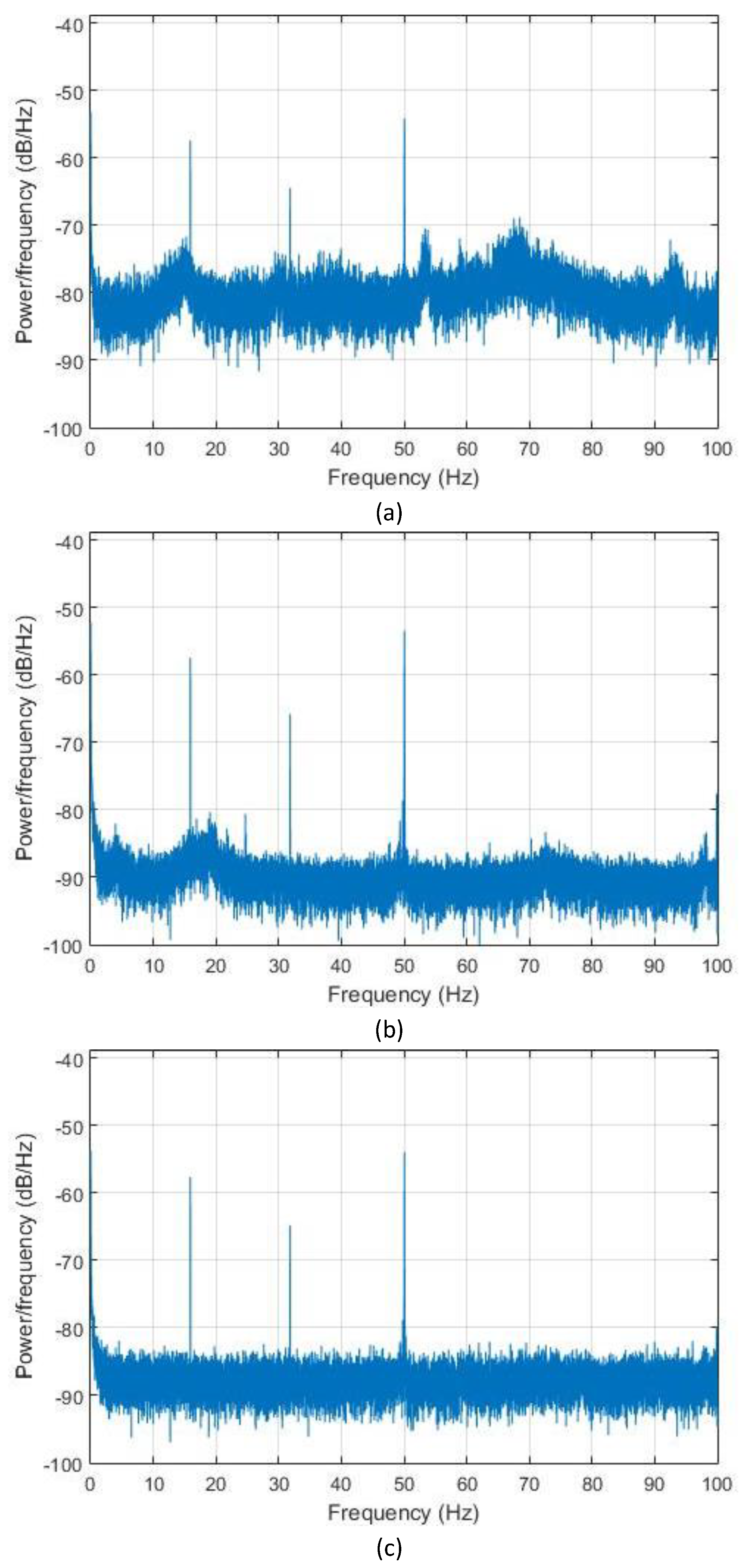
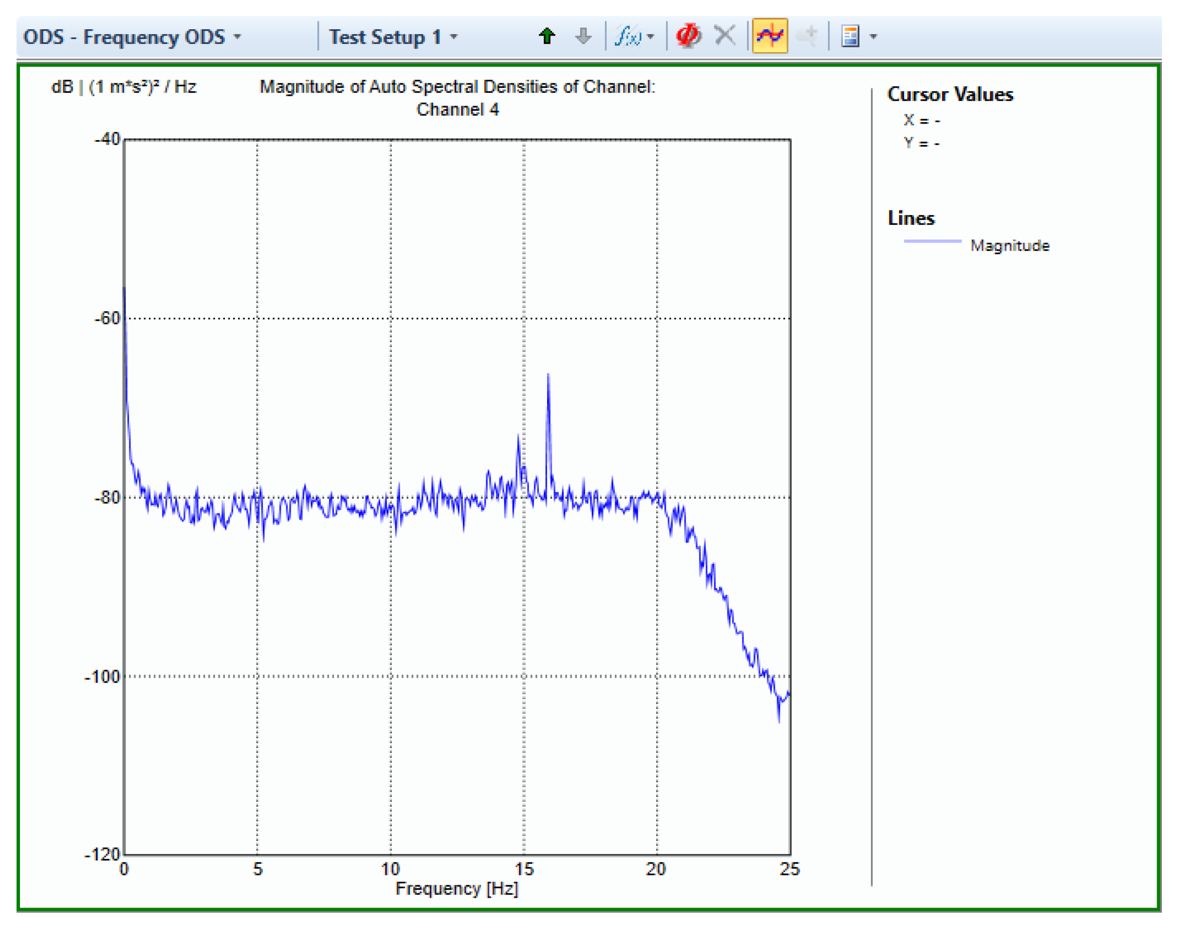
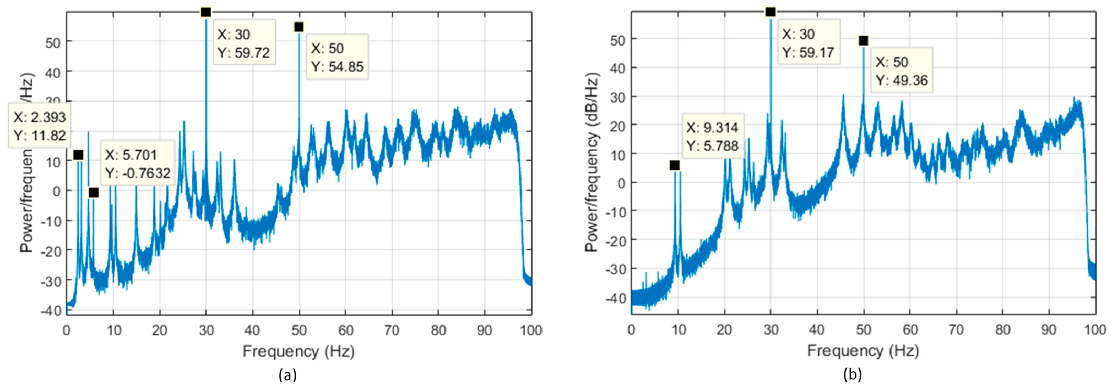
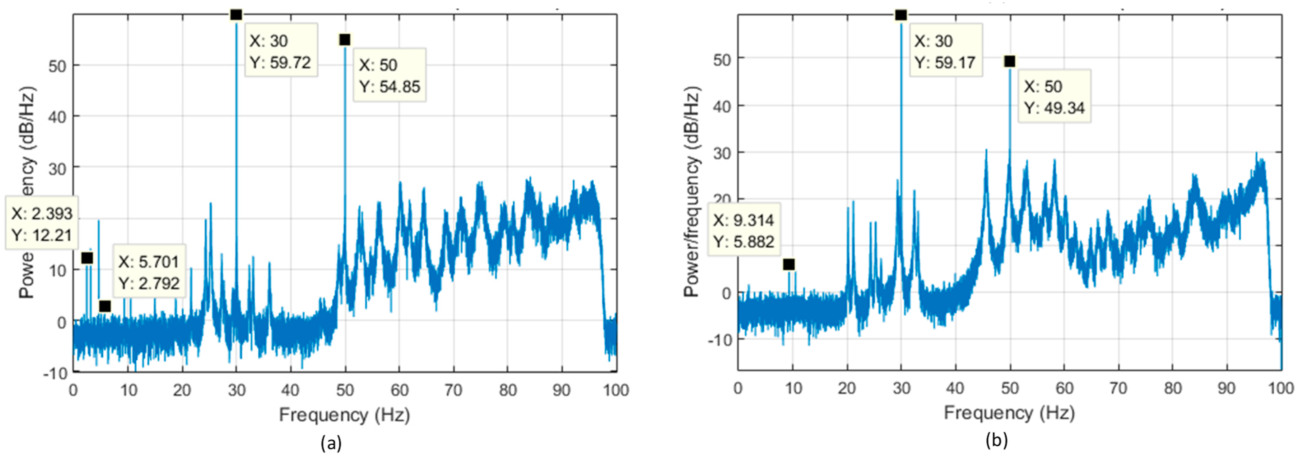
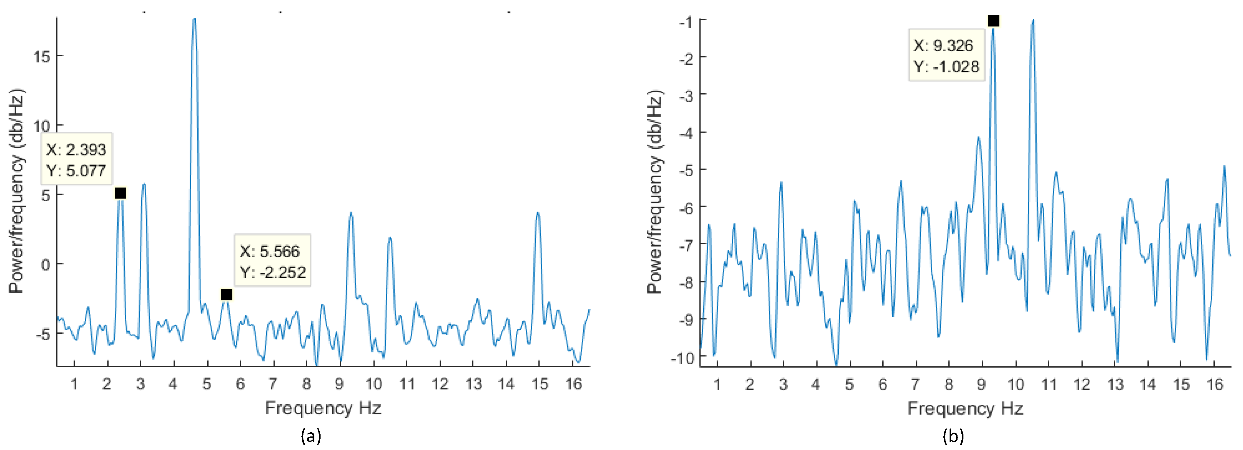
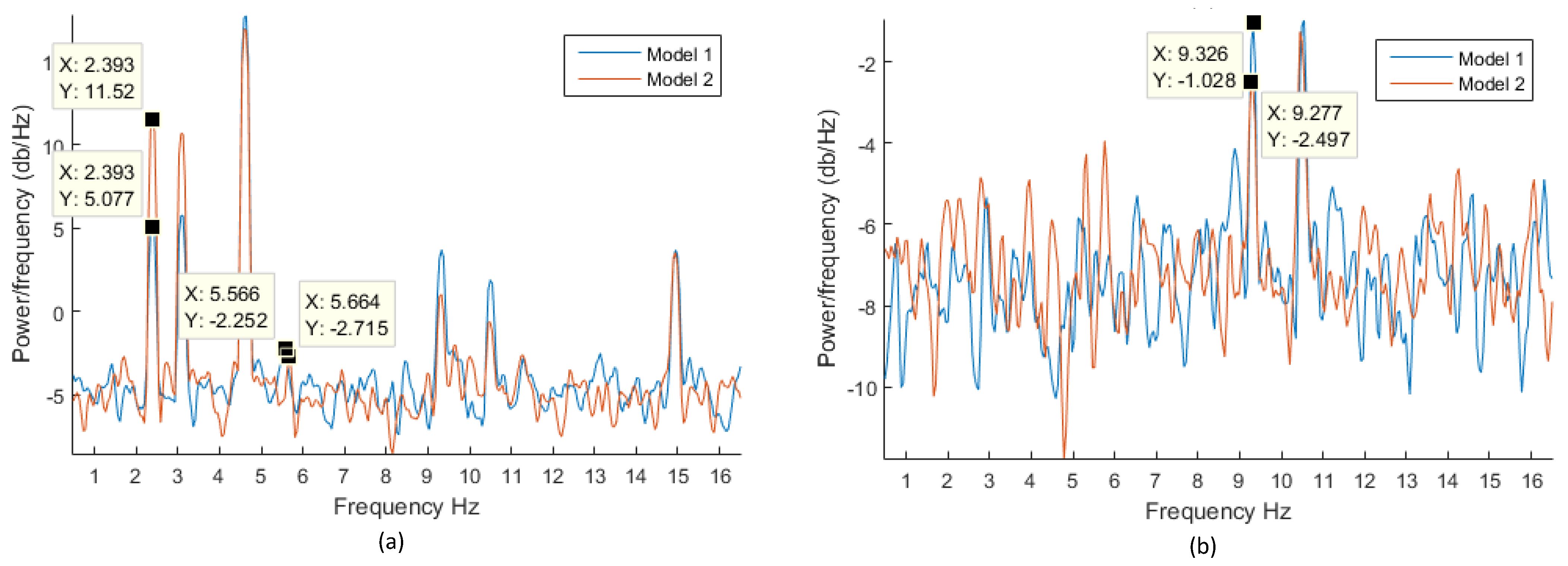
3.3. Power Spectral Density Analysis

To determine the experimental natural frequencies of the structure, data collected in the time domain by the three sensors were transformed into the frequency domain using Fourier Transform to evaluate the Power Spectral Densities (PSD) of each signal.
A MATLAB code was developed to generate the PSD of each channel and detect the peaks in the frequency range of structures by peak picking. The command pwelch was used with its default values, in which calculated segments had 50% overlap and were windowed with a Hamming window. Figure 10 shows the estimated PSD of all channels of Sensor B—as an example—for the total frequency range for the M2 measurement. It is worth noting that M1 results in almost identical graphs.
Every channel detected three peaks of 16 Hz, 30 Hz, and 50 Hz. The second and third frequencies were those of the motors in the adjacent factory (Figure 11). However, the first frequency of 16 Hz was too high to be the fundamental frequency of the structure, as this would indicate that the structure is much stiffer than expected.
The PSD was estimated within the normal frequency range of the structure, which was taken from zero to 20 Hz. However, the analysis of all channels in the reduced frequency range did not offer new information, which indicated that the peak-picking method might not be adequate to detect the natural frequencies of the structure and that other tools were needed.
Another tool adopting the FDD method was used for data analysis to explain the high frequencies detected previously. The ARTeMIS Modal software was used by utilising all its included methods, but no natural frequencies were detected. In addition, those methods did not identify any of the three peaks as natural frequencies, and, on the contrary, they were auto-detected as harmonic excitations. This result agrees with the explanation using the peak picking method where the frequencies appeared to be related to the operating frequencies of the motors of the neighbouring factory.
Figure 12 shows the estimated PSD of channel X of Sensor “B” of M1 using the FDD estimator, noting that the analysis of M2 measurement gave the same results. In this analysis, the data have been decimated to be between 0 and 25 Hz to be in the normal frequency range of structures, and the resolution was set to a value of 512 with zero percent overlap. Changing the estimator parameters did not also affect the spectral densities or the outcome of the analysis. Therefore, the above assessments did not result in an identification of the sought natural frequencies of the structure. The extraction of mode shapes appeared to be significantly affected by the level of noise within the data coupled with the existence of the neighbouring structure with operating motors. These aspects need to be investigated before using the MATLAB code. Therefore, numerical models were created for the purpose of assessing these effects and for verifying the MATLAB code before using it in the current analysis.

4. Dynamic Characterisation

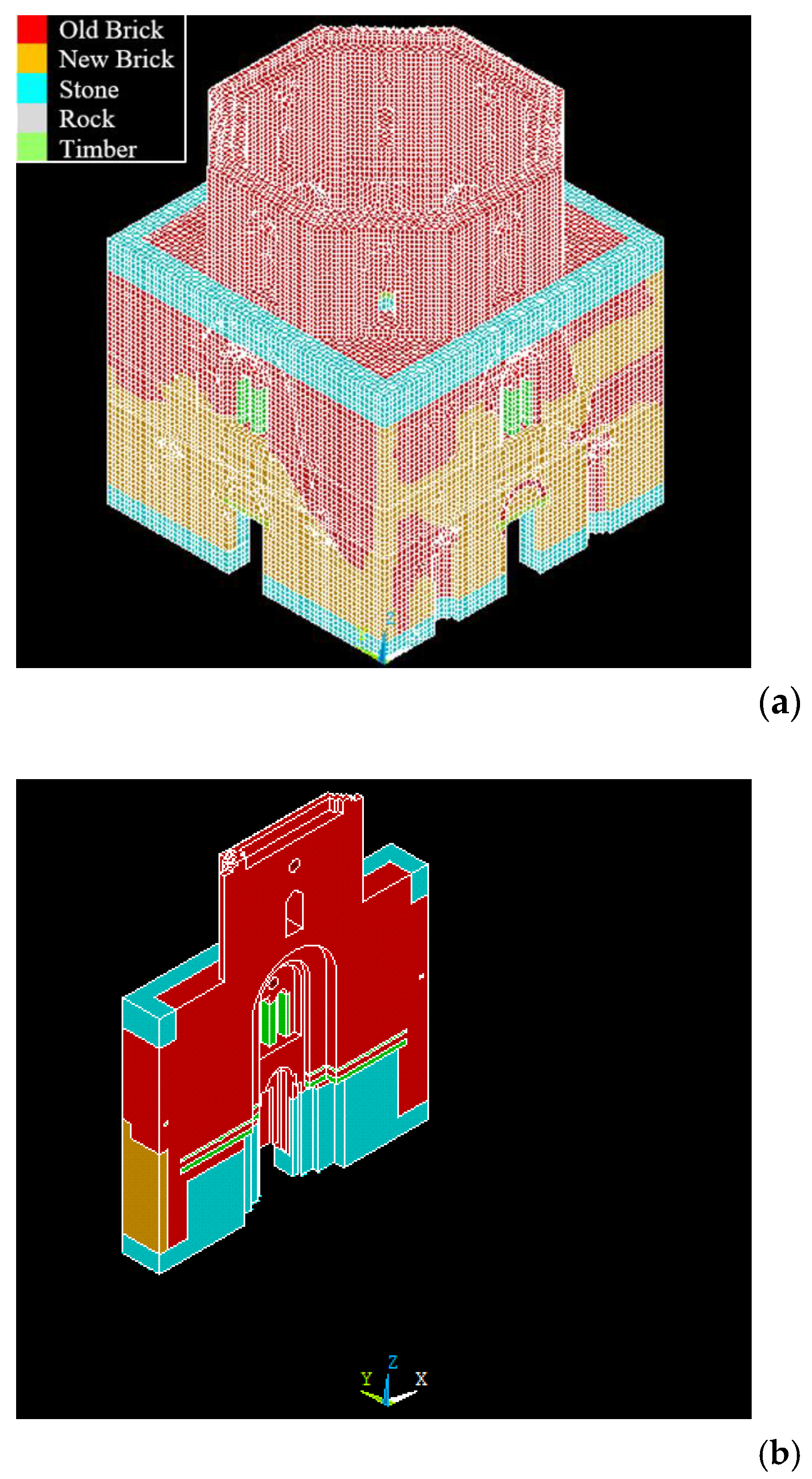
4.1. Numerical Modelling

4.1.1. Modelling Procedures

Model updating techniques are typically used to ensure compatibility between in situ dynamic testing and numerical simulations [51]. Refined finite element (FE) techniques using solid or shell elements and adopting various constitutive models are used to simulate the response of heritage masonry at the component or full-structure level [52,53]. Applied-element and discrete-element methods are also widely used for such purposes [54,55,56]. In this paper, the FE program ANSYS [55] was used for the structural analysis (Figure 13a). The numerical model was created using eight-node solid elements of type Solid65 with three displacement degrees of freedom at each node, as the structure is massive and has very thick walls. This element type also incorporates cracking and crushing capabilities, hence enabling future nonlinear inelastic assessments, but only the linear modal results are described herein. These results are typically used to evaluate the structural stiffness as a result of a change in the structure [42]. Table 1 summarises all the material properties adopted in the model. Because the current ceiling is not part of the original dome, it was excluded from the model. The foundation was assumed to be fixed to the ground in the linear model. According to the conversation plans by Megawra [38], there are variations in the material throughout the wall thickness of the dome, as shown in in Figure 13b.
From its geometry, it is evident that the structure is relatively stiff. This is verified by the modal analysis results, as the first mode identified had a frequency of 5.32 Hz. The first mode shape had a combination of movements in the x-direction and the y-direction, in which all perpendicular walls moved out of plane. The second and third modes had clear movements in the x-direction (Figure 14a) and the y-direction (Figure 14b), respectively, with close frequencies of 5.76 Hz and 5.9 Hz, respectively, due to the fact that the structure is almost doubly symmetric. The fourth mode had a similar movement to the first mode but for the corners of the perpendicular walls with a frequency of 6.49 Hz. The wall thickness in the corners was greater than in the middle; therefore, the four corners acted like four columns, and the mode shape involved free bending of each column as a cantilever in which each corner moves in the line connecting it to the opposite corner. Finally, torsion movements were clear in the fifth mode with a frequency of 9 Hz. Higher-order modes appeared after the fifth mode.
A complementary analysis on a skeletal model incorporating four perpendicular beams supported on four columns hinged at the base was also carried out to obtain insight into the dynamic response due to the vibrations arising from the adjacent factory. The model was subjected to very long excitation periods of 10 min using white noise to represent ambient vibrations simultaneously with harmonic excitations. In this model, the acceleration response was recorded at three points corresponding to the location of the physical accelerometers. Then, random noise was added to the acceleration response to represent the noise effects caused by the cables and the data acquisition system. Finally, in each case, the acceleration response was analysed using the MATLAB code and verified by modal analysis results using ANSYS.

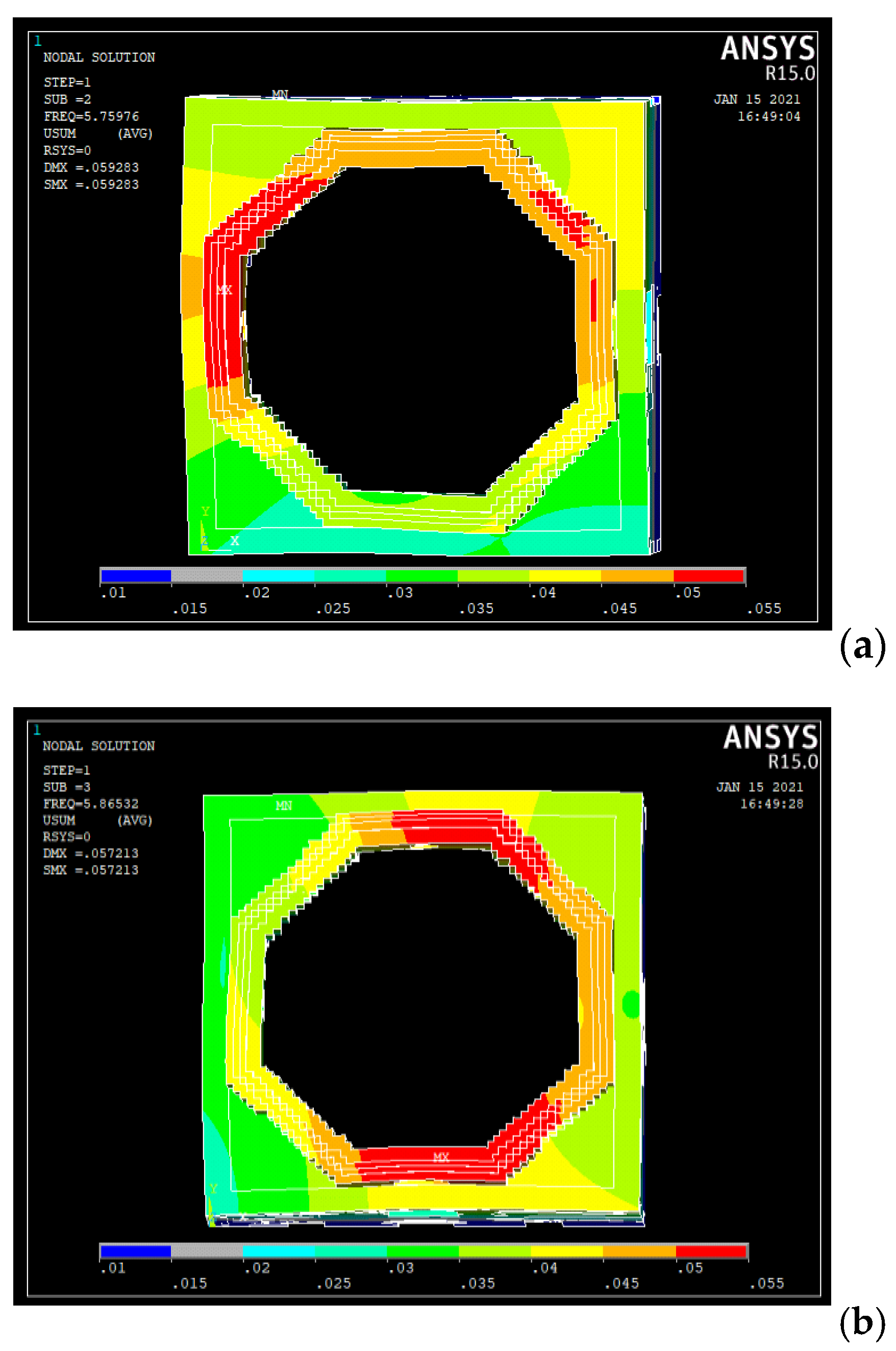
4.1.2. Modal Analysis

The natural frequencies computed from the numerical model are shown in Table 2. The target of the verification was to extract the same frequencies in this table from the experimental measurements after data-processing using MATLAB. In addition, the mode shapes were also verified by calculating the MAC value between the mode shapes given by ANSYS and those calculated by the MATLAB code, but the priority was given to the natural frequencies. Most of these modes act in the horizontal direction, such as the first two modes which are the translational modes in the x-direction and the y-direction. Other modes, such as Mode No 6, act in the vertical direction due to the deflection of the beams.
The numerical model was excited from its base using harmonic excitation at a frequency of 30 Hz in the x-direction and 50 Hz in the y-direction. Both directions were accompanied by white noise with an amplitude of 10 % of that of the harmonic excitation amplitude. The excitation continued for 10 min (600 s) with 0.005 s per step.
The acceleration response was recorded at three locations corresponding to the position of the physical accelerometers in the structure (Sensors 1, 2, and 3 were located at the corner and along the x-axis and the y-axis corresponding to B, D, and C positions shown in Figure 8). This means that the response simulates three tri-axial accelerometers located at these points, with a total of nine channels.

4.1.3. Evaluation Procedure

The Peak Picking method was used to determine the natural frequencies of the structure with the help of the pwelch command in MATLAB, employing the open-source codes for the calculations using FDD [45] and TDD [47] techniques.
The procedure followed included five steps. Firstly, the raw data were analysed as shown in Figure 15, such that all natural frequencies of the theoretical model were identified by the peaks in the graphs along with the two harmonic excitation frequencies, which are 30 Hz and 50 Hz. However, the amplitude of the white noise was only 10% of the harmonic excitation amplitude. This was enough to excite the natural frequencies of the structure. Accordingly, because the harmonic excitations from the neighbouring structure were of a different order of magnitude, they did not influence the natural frequencies of the structure. In Figure 15a, the second and fifth modes are pinned with frequencies of 2.393 Hz and 5.701 Hz, respectively; whereas in Figure 15b, the sixth mode is identified with a frequency of 9.314 Hz because this mode shape is mainly in the z-direction.
In the second step, 10% of random noise was added to the signal, then the new response was analysed again using the same technique. As shown in Figure 16a, the natural frequency of the second mode was identified by the peak picking method with the same frequency of 2.393 Hz, but the fifth mode was not clearly identified because of the added noise. In Figure 16b, the frequency of the sixth mode could be identified with the same frequency of 9.314 Hz. Subsequent steps were taken to identify the peaks which vanished due to the added noise such as the natural frequency of the fifth mode.
In the third step, the frequency range was decreased to focus only on the region where the natural frequencies of the structure occurred, which is below 16 Hz; however, it was not possible to identify the fifth mode. This was followed by the fourth step, in which the default values of the pwelch command were changed to generate smoother curves. Flat Top window was used to focus on the amplitude of the peaks and differentiate between them and the peaks due to added noise. In addition, the window size was reduced to 20 s to increase the number of segments to enhance the averaging between them, where the noise effect is cancelled out by taking more average values, but the decrease in windows size decreases the accuracy of the corresponding frequency for each peak.
The effect of changing the default values to the specified values smoothed the curves, as shown in Figure 17, with a decrease in the accuracy such that the fifth mode was identified with a frequency of 5.566 Hz instead of 5.701 Hz. The fifth mode was then detected as a local peak, as shown in Figure 17a, but it still needed another verification to prove that it is a global peak and represents a natural frequency of the structure.
Using the same comparison procedure provided by Sun and Büyüköztürk [28], this local peak may be detected as a global peak if there exists another measurement of the structure with the same local peak. Therefore, another excitation to the theoretical model was performed using the same harmonic excitation in the x- and y-directions, using a different white noise excitation with the previous amplitude ratio to simulate another measurement carried out under different ambient conditions. This means that there are now two theoretical models.
The analysis of the two models is shown and compared in Figure 18a in the x-direction, in which the local peaks at the frequencies of 5.566 Hz for the first model and 5.664 Hz for the second model are repeated; whereas other local peaks are not repeated along the frequency domain. Thus, this local peak can be detected as a natural frequency of the structure because it has been repeated in the two models. In addition to the fifth mode, the peaks of the second mode exist in the two models, which confirms that it represents a natural frequency of the structure. The same conclusion can be achieved for the sixth mode by comparing the two models in the z-direction, as shown in Figure 18b, in which the detected peaks of the sixth mode are the same in the two models.
At each selected peak, the mode shape was calculated for the pure and the noisy records of the two excitations using the FFT method, FDD technique, and the TDD technique with a comparison between the calculated mode shapes and the theoretical ones by calculating the MAC value, as summarised in Table 3. The FDD and TDD methods showed stable MAC values for the pure and the noisy records, with a minimum of 0.922 and 0.966 for the two techniques, respectively. However, it was not possible to determine the mode shapes for the noisy record using the FFT method, in which the MAC value was 0.354 for the fifth mode for one of the two noisy excitations.

4.2. Signal Processing

During the previous signal processing of the data, the natural peaks of the theoretical model were successfully detected through the following procedure: firstly, the separation of the registered channels according to the calculated mode shapes; secondly, the use of the Flat Top window function with 2 s window size; and finally, the comparison between the two different measurements.
It was possible to apply the above-described procedure to the data, as two different measurements have been recorded for the structure with different registration times. These two records were denoted M1 and M2 with a registration time of about 10   m i n s and 20 min, respectively. In addition, three modes out of the five numerical modes have unique active channels that can be registered simultaneously during signal processing, in which the second mode has active channels in the x-direction, which might be referred to as the transitional X mode, the third mode has active channels in the y-direction and can be referred to the transitional Y mode, and the fifth mode has active channels in both the x- and the y-directions and can represent the torsional mode. The other two modes do not have unique channels along one or two directions, which make them more difficult to assess.
In the following subsections, the previous approach is applied to the signal processing of the two measurements to detect the natural frequencies and mode shapes of the structure.

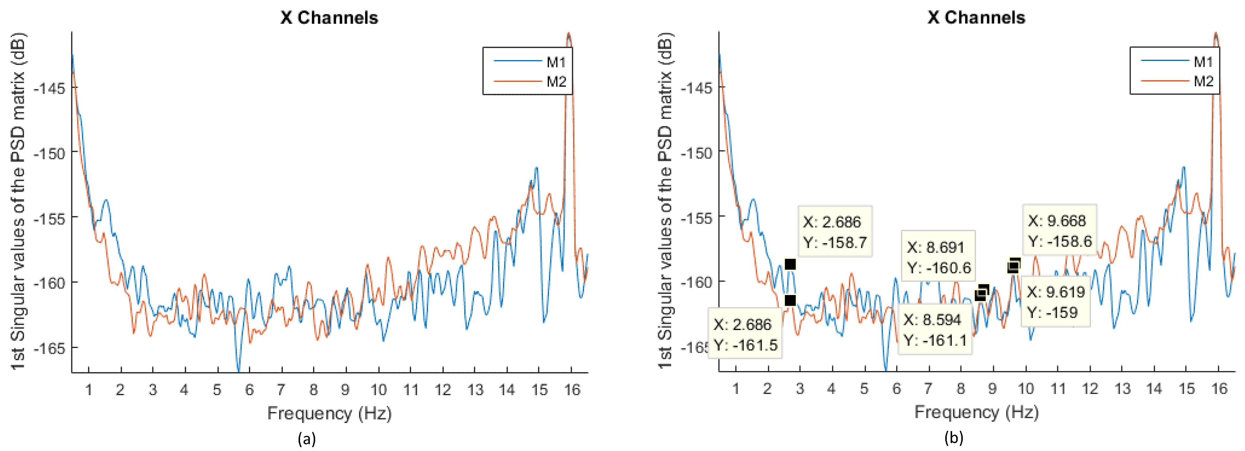
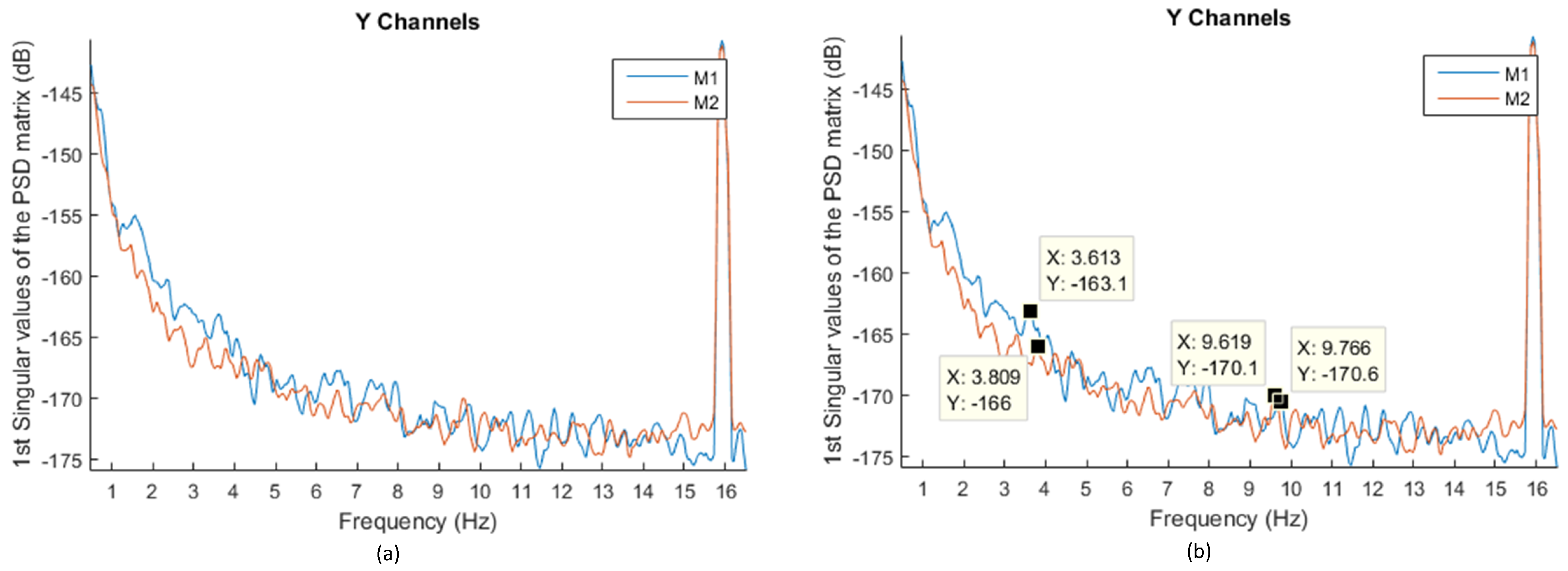
4.2.1. Natural Frequencies

To detect the Transitional X mode, only the X channels were used during the analysis, as shown in Figure 19a. By comparing the local peaks of the two measurements, three repeated peaks could be found in the two measurements, as shown in Figure 19b. The first peak was detected at a frequency of 2.686 Hz at the two measurements, which indicates a natural frequency of the structure at this value and means that the Transitional X mode was detected with a value of 2.686 Hz. Due to the lower accuracy obtained by decreasing the window size, this value might be inaccurate, and a minimum and a maximum value should be considered around the peak, which were selected as 2.60 Hz and 2.75 Hz, respectively. The other two detected peaks could be related to other mode shapes that share the X channels, such as the torsion mode; thus, these two values may appear later during the analysis of the torsion mode.
For the Transitional Y mode, only the channels in the y-direction have been used for generating the PSD, as shown in Figure 20a. The local peaks of the two measurements are selected for each measurement and compared in Figure 20b. Again, three local peaks are repeated in the two measurements, whereas the first peak has a slight difference in the two measurements with a frequency of 3.613 Hz and 3.809 Hz for M1 and M2, respectively. This means that the natural frequency of the Transitional Y mode was detected as 3.6 Hz with a minimum and a maximum value of 3.3 Hz and 3.9 Hz, respectively. These values are rounded because the local peaks are not identical in the two measurements, whereas the minimum value has been selected according to the local peak of M2. This means that the selected peak is taken from M1, whereas the range is selected by the other two peaks of M2 surrounding M1.
The other two detected peaks might be peaks regarding other modes that share the y-direction channels, such as the torsion mode, which means it might appear in the PSD during detection of the peaks of the torsion mode. Finally, the channels contributing to the other modes, such as the torsion mode, were analysed simultaneously. Thus, the channels in the x- and y-directions are used for generating the PSD. With a similar argument as the one discussed above, three peaks were detected. Two of these peaks appeared before during the analysis of the channels in the x-direction only and the channels in the y-direction only, which proves that these modes are related to other mode shapes in which the channels in the x- and y-directions have a significant contribution to the mode, which is the case in the torsion mode. The three peaks lie in the interval between 8.5 Hz and 10 Hz for M1 and M2 with the focus on the peak with the most amplitude with a frequency of 9.619 Hz and 9.668 Hz for M1 and M2, respectively. Thus, the selected frequency is taken as 9.65 Hz.
Table 4 provides the selected natural frequency associated with each mode shape with a minimum and maximum value for the natural frequency for each mode. The detected modes are the Transitional X mode, the Transitional Y mode, and the torsion mode, all of which have the most mass participation ratio relative to the other modes, such as the other two undetected modes.

4.2.2. Frequencies and Damping Ratios

For each detected mode at the selected frequency, the corresponding mode shape has been calculated using the TDD [49] technique, which was very stable during the determination of the mode shapes of the noisy records of the validation model. Accordingly, MAC values were calculated for the second measurement relative to the initial numerical model, which are 0.978, 0.947, and 0.254 for the Transitional X mode, the Transitional Y mode, and the torsion mode, respectively.
Because this technique does not provide the damping ratios, the AFDD [49] technique was used to calculate the damping rations for each detected mode shape. The analysis of M1 gave damping ratios of 4.7%, 5.0%, and 4.7% for the Transitional X mode, the Transitional Y mode, and the torsion mode, respectively. The analysis of M2 resulted in damping ratios of 4.9%, 5.0%, and 4.5% for the Transitional X mode, the Transitional Y mode, and the torsion mode, respectively. The values are close to each other for the two measurements, with the same average of all modes of 4.9%. The average values between the two measurements of each mode are reported in Table 4.
As described in this study, only one setup was utilised for the dynamic investigation tests due to inaccessibility issues which led to extracting data from a small part of the structure at just three nearby points located at the same level. The configuration caused some difficulties during the Power spectral density (PSD) analysis, which did not enable direct capturing of the dynamic properties of the structure. Noise in the signal, appearing at the same frequency for different measurements, also posed challenges in evaluating the true natural frequencies of the structure. The approach proposed in this paper successfully detected the natural frequencies of the heritage structure by using a theoretical validation model that was excited by white noise, along with operating high frequencies. After smoothing the PSD curves using windowing, the comparison between the measurements identified the true peaks in the signal, appearing in both measurements. A false peak would occur in one measurement but not in the second.
It was shown that the operating high frequencies have no effect on the spectral analysis through the normal range of the natural frequencies of the structure. If the operational frequencies were in that range, it might cause problems in detecting the natural frequencies using the peak-picking method. Over-smoothing of the PSD curves might cause one peak not to coincide with another peak during the comparison of the results. This occurs due to the averaging nature of the smoothing window. Therefore, a range of selected peaks should be provided rather than reporting one value, as given in Table 4, because this range depends on the extent of smoothing and how well the two peaks coincide during the comparison step. The window size can be determined during the analysis of the validation model.
The proposed approach was able to detect the natural frequencies of three global modes of the dome in agreement with the MAC values, with two of them resembling those from the numerical model. The third mode is torsion-related and cannot be determined while all the sensors are located at only one corner of the structure. In order to capture this mode shape, and in situations in which accessibility is possible, another setup with sensors in two opposite corners of the structure would be needed.
As described before, the detected experimental frequencies are lower than those obtained from the numerical models. This indicates that additional sources of flexibility exist in the structure, which are primarily attributed to possible soil–structure interaction effects, which are not captured by the idealised foundation support conditions assumed in modelling. The experimental measurements obtained can, therefore, be used to calibrate the models in future studies with due account for soil flexibility. Overall, the proposed approaches for identifying the key natural frequencies can be of direct use in similar situations in which there is limited accessibility to the structure.

5. Conclusions

The paper presented an investigation into the dynamic characteristics of a historical structure employing both experimental modal analysis and finite element modelling. A numerical model was created employing available architectural and material data, site measurements, and in situ testing to obtain insight into the dominant modes of vibration. To assess the actual characteristics of the structure, a number of dynamic tests and complementary analyses were carried out. Due to severe accessibility issues, the instrumentation was installed in only a small part of the structure at one level. To deal with these limitations in the instrumentation set-up, an approach was proposed in this paper to enable the identification of the dynamic properties of the structure.
One of the main steps of this approach is to select the channels that contribute to specific modes. For example, the channels in the x-direction were used to generate a spectral density figure in order to capture the transitional mode in the x-direction. Appropriate choice of the parameters of the signal-processing procedure was discussed to generate smooth graphs that can be compared together. This comparison between the generated graphs provided necessary cross validation, as it was difficult to differentiate between the noise and the natural frequencies of the structure using only one resulting history.
Using the proposed approach for the signal processing utilising the MATLAB code, the captured modes were transitional in the x-direction; transitional in the y-direction; and torsional modes with frequencies of 2.686 Hz, 3.6 Hz, and 9.65 Hz, respectively, and corresponding damping ratios of 4.8%, 5.0%, and 4.6%, respectively. However, despite the localised setup problem and the restricted allocation of sensors, the MALTAB code enabled the extraction of three modes of the structure.
The validation model was used to compare the different methods adopted in this analysis to calculate the MAC value between the experimental and the numerical mode shapes. The FFT method was affected by the presence of noise, whereas the most stable method was TDD. The latter depends on the time domain of the measurement without the need to transform the response into the frequency domain before calculations. Therefore, in this study, TDD was selected and employed for the analysis of the measurements of the structure.
It was also shown that the interference from the neighbouring factory had a minimal effect on the signal processing, because the operating frequencies were found to be sufficiently distant from the natural frequencies of the structure. The approaches proposed in this paper, including identification of the key natural frequencies, inform and direct structural restoration for the structure and can be used for other heritage structures located in congested historic sites.

Author Contributions

Conceptualisation, S.A.M., A.E. and A.G.E.-A.; methodology, S.A.M., A.E. and A.G.E.-A.; software, A.R.B.; formal analysis, A.R.B.; investigation, A.R.B.; writing—original draft preparation, A.R.B.; writing—review and editing, A.Y.E. and D.V.B.; supervision, S.A.M., A.E. and A.G.E.-A.; funding acquisition, S.A.M. and A.Y.E. All authors have read and agreed to the published version of the manuscript.

Funding

This work was supported by the Science, Technology and Innovation Funding Authority (STIFA) of Egypt under Grant No. AHRC30799 and the Arts and Humanities Research Council (AHRC) of the UK under Grant No. AH/R00787X/1.

Data Availability Statement

Data may be made available on request.

Acknowledgments

This study was carried out within the research project “Interdisciplinary approach for the management and conservation of UNESCO World Heritage Site of Historic Cairo-Application to Al-Ashraf Street”. The financial support of STIFA/AHRC is gratefully acknowledged.

Conflicts of Interest

The authors declare no conflict of interest.

References

  1. Stepinac, M.; Gašparović, M. A Review of Emerging Technologies for an Assessment of Safety and Seismic Vulnerability and Damage Detection of Existing Masonry Structures. Appl. Sci. 2020, 10, 5060. [Google Scholar] [CrossRef]
  2. Moretić, A.; Stepinac, M.; Lourenço, P.B. Seismic upgrading of cultural heritage—A case study using an educational building in Croatia from the historicism style. Case Stud. Constr. Mater. 2022, 17, e01183. [Google Scholar] [CrossRef]
  3. Boscato, G.; Fragonara, L.Z.; Cecchi, A.; Reccia, E.; Baraldi, D. Structural Health Monitoring through Vibration-Based Approaches. Shock. Vib. 2019, 2019, 2380616. [Google Scholar] [CrossRef]
  4. Ceravolo, R.; Pistone, G.; Fragonara, L.Z.; Massetto, S.; Abbiati, G. Vibration-Based Monitoring and Diagnosis of Cultural Heritage: A Methodological Discussion in Three Examples. Int. J. Arch. Herit. 2014, 10, 375–395. [Google Scholar] [CrossRef] [Green Version]
  5. Lorenzoni, F.; Casarin, F.; Modena, C.; Caldon, M.; Islami, K.; da Porto, F. Structural health monitoring of the Roman Arena of Verona, Italy. J. Civ. Struct. Heal. Monit. 2013, 3, 227–246. [Google Scholar] [CrossRef]
  6. Masciotta, M.-G.; Ramos, L.F.; Lourenço, P.B. The importance of structural monitoring as a diagnosis and control tool in the restoration process of heritage structures: A case study in Portugal. J. Cult. Herit. 2017, 27, 36–47. [Google Scholar] [CrossRef] [Green Version]
  7. Chiorino, M.A.; Ceravolo, R.; Spadafor, A.; Fragonara, L.Z.; Abbiati, G. Dynamic Characterization of Complex Masonry Structures: The Sanctuary of Vicoforte. Int. J. Arch. Herit. 2011, 5, 296–314. [Google Scholar] [CrossRef]
  8. Pieraccini, M.; Dei, D.; Betti, M.; Bartoli, G.; Tucci, G.; Guardini, N. Dynamic identification of historic masonry towers through an expeditious and no-contact approach: Application to the “Torre del Mangia” in Siena (Italy). J. Cult. Herit. 2014, 15, 275–282. [Google Scholar] [CrossRef]
  9. Russo, S. Integrated assessment of monumental structures through ambient vibrations and ND tests: The case of Rialto Bridge. J. Cult. Herit. 2016, 19, 402–414. [Google Scholar] [CrossRef]
  10. Ivorra, S.; Pallarés, F.J. Dynamic investigations on a masonry bell tower. Eng. Struct. 2006, 28, 660–667. [Google Scholar] [CrossRef]
  11. Saisi, A.; Gentile, C. Post-earthquake diagnostic investigation of a historic masonry tower. J. Cult. Herit. 2015, 16, 602–609. [Google Scholar] [CrossRef]
  12. Ramos, L.; De Roeck, G.; Lourenco, P.; Campos-Costa, A. Damage identification on arched masonry structures using ambient and random impact vibrations. Eng. Struct. 2010, 32, 146–162. [Google Scholar] [CrossRef]
  13. Azzara, R.M.; Girardi, M.; Iafolla, V.; Lucchesi, D.M.; Padovani, C.; Pellegrini, D. Ambient Vibrations of Age-old Masonry Towers: Results of Long-term Dynamic Monitoring in the Historic Centre of Lucca. Int. J. Arch. Herit. 2019, 15, 5–21. [Google Scholar] [CrossRef] [Green Version]
  14. Diz-Mellado, E.; Mascort-Albea, E.J.; Romero-Hernández, R.; Galán-Marín, C.; Rivera-Gómez, C.; Ruiz-Jaramillo, J.; Jaramillo-Morilla, A. Non-destructive testing and Finite Element Method integrated procedure for heritage diagnosis: The Seville Cathedral case study. J. Build. Eng. 2021, 37, 102134. [Google Scholar] [CrossRef]
  15. Funari, M.F.; Silva, L.C.; Mousavian, E.; Lourenço, P.B. Real-time Structural Stability of Domes through Limit Analysis: Application to St. Peter’s Dome. Int. J. Arch. Herit. 2021, 1–23. [Google Scholar] [CrossRef]
  16. Hemeda, S. 3D finite element coupled analysis model for geotechnical and complex structural problems of historic masonry structures: Conservation of Abu Serga church, Cairo, Egypt. Heritage Sci. 2019, 7, 6. [Google Scholar] [CrossRef] [Green Version]
  17. Ewins, D.J. Modal Testing: Theory and Practice; Wiley: Hoboken, NJ, USA, 1984. [Google Scholar]
  18. Bartoli, G.; Betti, M.; Giordano, S. In situ static and dynamic investigations on the “Torre Grossa” masonry tower. Eng. Struct. 2013, 52, 718–733. [Google Scholar] [CrossRef]
  19. Magalhães, F.; Cunha, Á. Explaining operational modal analysis with data from an arch bridge. Mech. Syst. Signal Process. 2011, 25, 1431–1450. [Google Scholar] [CrossRef] [Green Version]
  20. Zini, G.; Betti, M.; Bartoli, G.; Chiostrini, S. Frequency vs time domain identification of heritage structures. Procedia Struct. Integr. 2018, 11, 460–469. [Google Scholar] [CrossRef]
  21. Elyamani, A.; Roca Fabregat, P. A review on the study of historical structures using integrated investigation activities for seismic safety assessment. Part I: Dynamic investigation. Sci. Cult. 2018, 4, 1–27. [Google Scholar] [CrossRef]
  22. Boscato, G.; Reccia, E.; Cecchi, A. Non-destructive experimentation: Dynamic identification of multi-leaf masonry walls damaged and consolidated. Compos. Part B Eng. 2018, 133, 145–165. [Google Scholar] [CrossRef]
  23. Fragonara, L.Z.; Boscato, G.; Ceravolo, R.; Russo, S.; Ientile, S.; Pecorelli, M.L.; Quattrone, A. Dynamic investigation on the Mirandola bell tower in post-earthquake scenarios. Bull. Earthq. Eng. 2016, 15, 313–337. [Google Scholar] [CrossRef] [Green Version]
  24. De Angelis, A.; Lourenço, P.B.; Sica, S.; Pecce, M.R. Influence of the ground on the structural identification of a bell-tower by ambient vibration testing. Soil Dyn. Earthq. Eng. 2022, 155, 107102. [Google Scholar] [CrossRef]
  25. Russo, S.; Spoldi, E. Damage assessment of Nepal heritage through ambient vibration analysis and visual inspection. Struct. Control. Health Monit. 2020, 27, e2493. [Google Scholar] [CrossRef]
  26. Lithgow, R.; Whittaker, S.; Bower, T.; Corda, K.; Woolley, E.; Higgitt, C.; Vlachou-Mogire, C.; Babington, C. Vibration Monitoring of Daniel Maclise’s Wall Painting Trafalgar. Stud. Conserv. 2020, 65, P180–P186. [Google Scholar] [CrossRef]
  27. Gentile, C.; Ruccolo, A.; Saisi, A. Continuous Dynamic Monitoring to Enhance the Knowledge of a Historic Bell-Tower. Int. J. Arch. Herit. 2019, 13, 992–1004. [Google Scholar] [CrossRef]
  28. Sun, H.; Büyüköztürk, O. The MIT Green Building benchmark problem for structural health monitoring of tall buildings. Struct. Control. Heal. Monit. 2017, 25, e2115. [Google Scholar] [CrossRef]
  29. Aktaş, Y.D.; Turer, A. Seismic evaluation and strengthening of nemrut monuments. J. Cult. Herit. 2015, 16, 381–385. [Google Scholar] [CrossRef]
  30. Martínez-Soto, F.; Ávila, F.; Puertas, E.; Gallego, R. Spectral analysis of surface waves for non-destructive evaluation of historic masonry buildings. J. Cult. Herit. 2021, 52, 31–37. [Google Scholar] [CrossRef]
  31. UK Research and Innovation: Interdisciplinary Approach for the Management and Conservation of UNESCO World Heritage Site of Historic Cairo. Application to Al-Ashraf Street. 2019. Available online: https://gtr.ukri.org/projects?ref=AH%2FR00787X%2F1 (accessed on 7 July 2019).
  32. Elghazouli, A.Y.; Bompa, D.V.; Mourad, S.A.; Elyamani, A. In-plane lateral cyclic behaviour of lime-mortar and clay-brick masonry walls in dry and wet conditions. Bull. Earthq. Eng. 2021, 19, 5525–5563. [Google Scholar] [CrossRef]
  33. Bakkar, A.R. Numerical Modelling and System Identification of a Historic Masonry Structure in Historic Cairo Using Dynamic Investigation Tests. Master’s Thesis, Cairo University, Cairo, Egypt, 2021. [Google Scholar]
  34. Elghazouli, A.Y.; Bompa, D.V.; Mourad, S.A.; Elyamani, A. Structural behaviour of clay brick lime mortar masonry walls under lateral cyclic loading in dry and wet conditions. In Proceedings of the International Conference on Protection of Historical Constructions, Athens, Greece, 25–27 October 2021; Springer: Cham, Switzerland, 2021; pp. 164–174. [Google Scholar] [CrossRef]
  35. Williams, C. Islamic Monuments in Cairo: The Practical Guide; American University in Cairo Press: Cairo, Egypt, 2008. [Google Scholar]
  36. Elghazouli, A.Y.; Bompa, D.V.; Mourad, S.A.; Elyamani, A. Seismic Performance of Heritage Clay Brick and Lime Mortar Masonry Structures. In European Conference on Earthquake Engineering and Seismology; Springer: Cham, Switzerland, 2022; pp. 225–244. [Google Scholar] [CrossRef]
  37. Sonbol, A. Beyond the Exotic: Women’s Histories in Islamic Societies; Syracuse University Press: Syracuse, NY, USA, 2005. [Google Scholar]
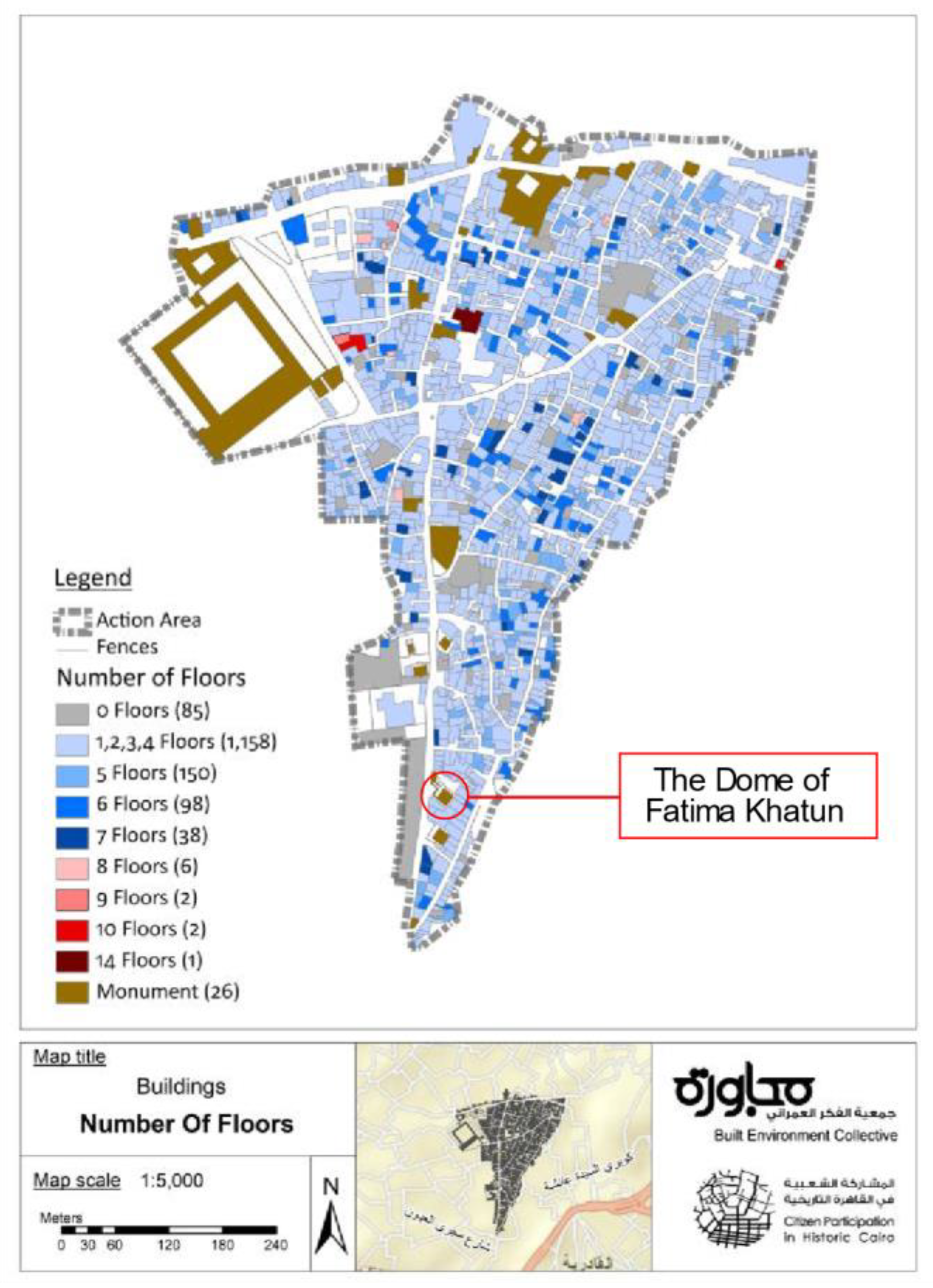
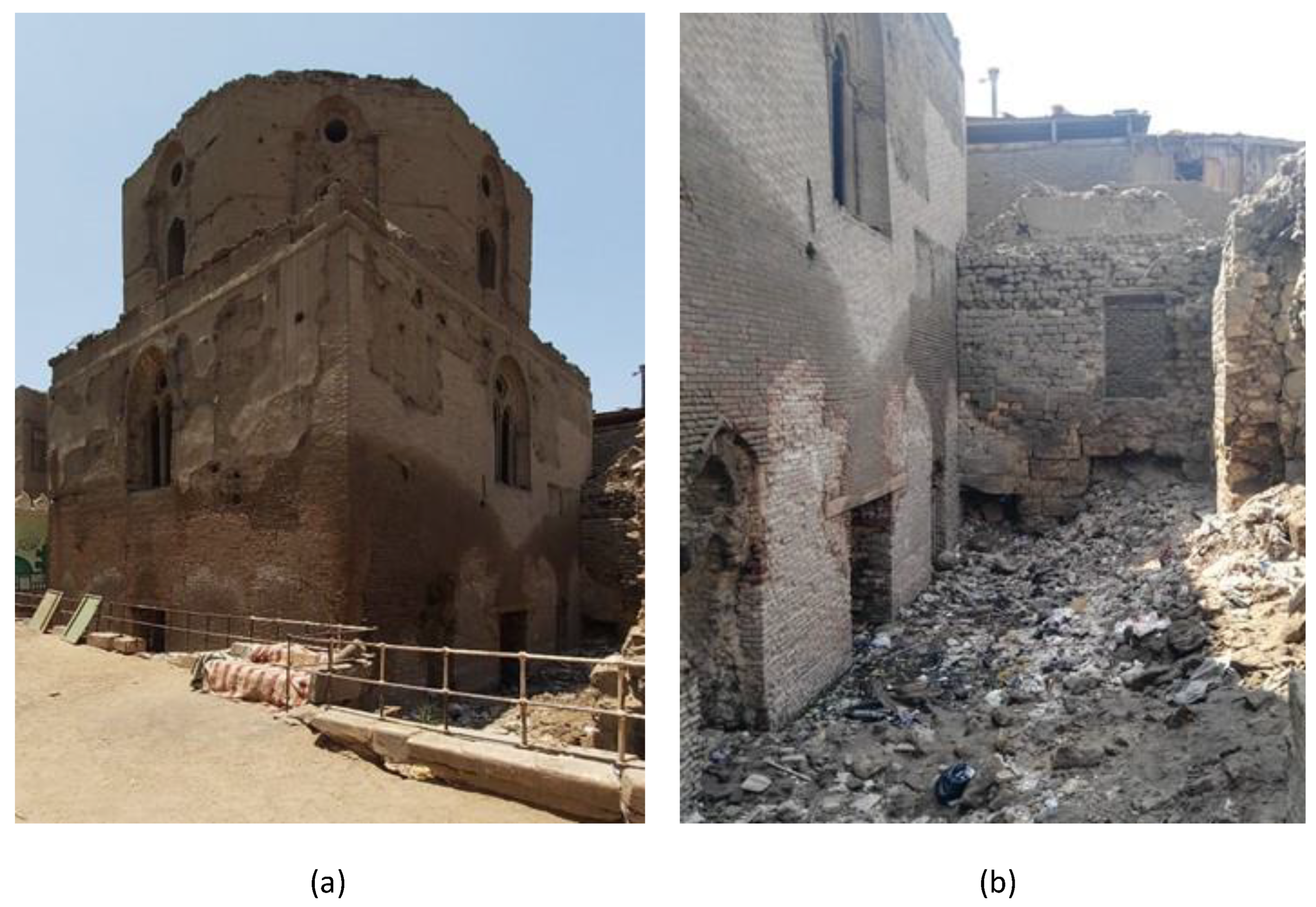
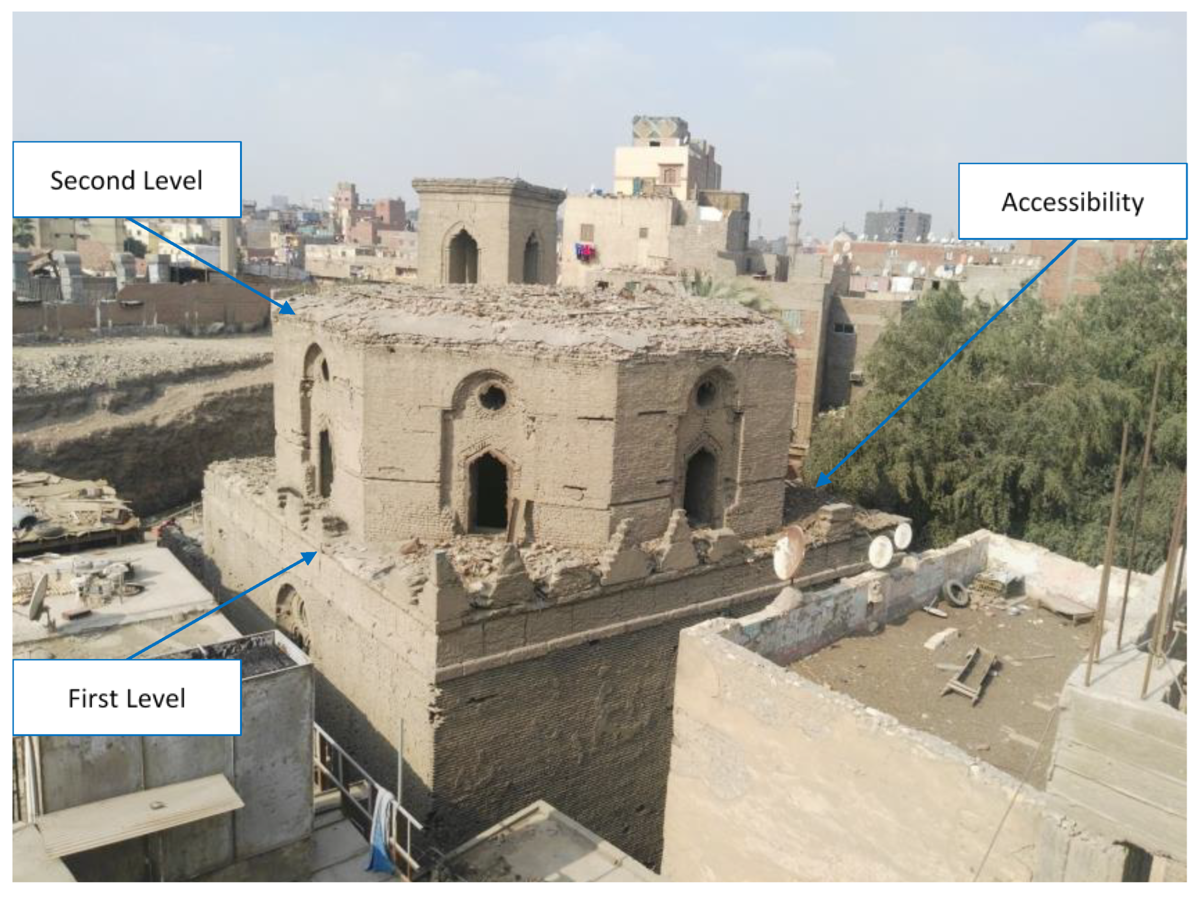
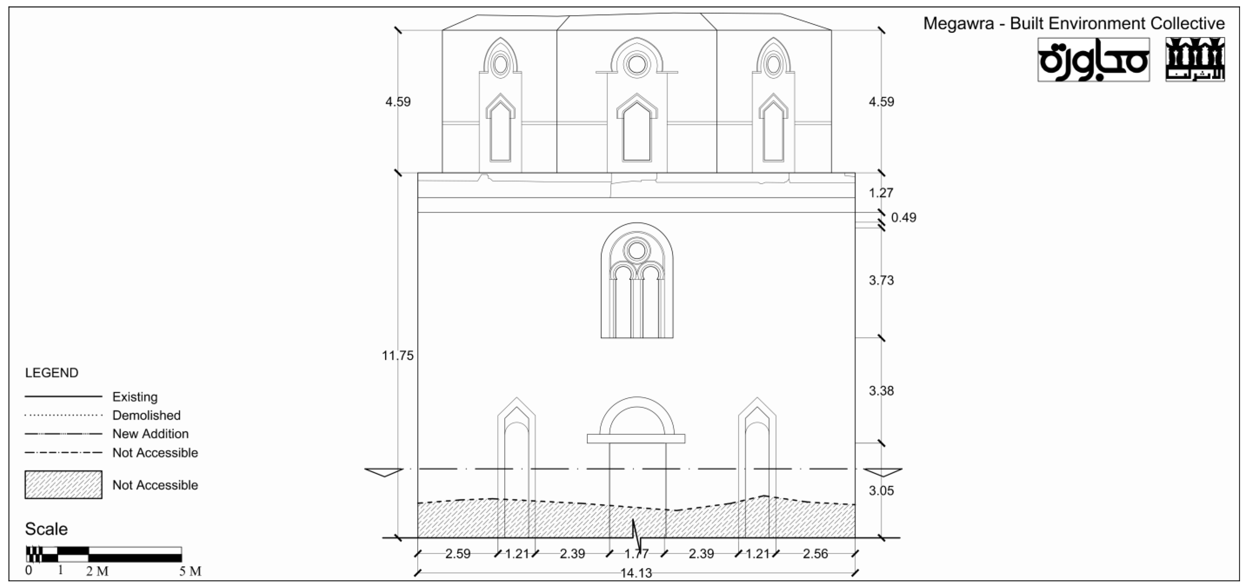
  38. Megawra-BEC (Megawra Built Environment Collective). The Dome of Fatima Khatun; Megawara-BEC: Cairo, Egypt, 2017. [Google Scholar]
  39. Megawra-BEC (Megawra Built Environment Collective). Al-Khalifa Updated Maps; Megawara-BEC: Cairo, Egypt, 2017. [Google Scholar]
  40. Buttkus, B. Spectral Analysis and Filter Theory in Applied Geophysics; Springer Science & Business Media: Berlin/Heidelberg, Germany, 2012. [Google Scholar] [CrossRef]
  41. Welch, P.D. The use of fast Fourier transform for the estimation of power spectra: A method based on time averaging over short, modified periodograms. IEEE Trans. Audio Electroacoust. 1967, 15, 70–73. [Google Scholar] [CrossRef] [Green Version]
  42. Zaknich, A. Principles of Adaptive Filters and Self-Learning Systems; Springer International Publishing: Berlin/Heidelberg, Germany, 2005. [Google Scholar]
  43. MATLAB. R2015a; The MathWorks, Inc.: Natick, MA, USA, 2015. [Google Scholar]
  44. Understanding FFTs and Windowing. 2019. Available online: https://download.ni.com/evaluation/pxi/Understanding%20FFTs%20and%20Windowing.pdf (accessed on 8 January 2023).
  45. Farshchin, M. Frequency Domain Decomposition (FDD). MATLAB Central File Exchange. 2020. Available online: https://www.mathworks.com/matlabcentral/fileexchange/50988-frequency-domain-decomposition-fdd. (accessed on 29 November 2020).
  46. Cheynet, E. Automated Frequency Domain Decomposition (AFDD). Zenodo. 2020. Available online: https://zenodo.org/record/4277622 (accessed on 29 November 2020).
  47. Cheynet, E. Mode Shapes Extraction by Time Domain Decomposition (TDD). GitHub. 2020. Available online: https://github.com/ECheynet/TDD/releases/tag/v2.5 (accessed on 29 November 2020).
  48. ARTeMIS Modal. 6.1; Structural Vibration Solutions: Aalborg, Denmark, 2019.
  49. MACEC. 3.3; Structural Mechanics Section of KU Leuven: Leuven, Belgium, 2014.
  50. EpiSensor Model FBA ES-T; Kinemetrics: Pasadena, CA, USA, 2022.
  51. Ozcelik, O.; Misir, I.S.; Yucel, U.; Durmazgezer, E.; Yucel, G.; Amaddeo, C. Model updating of Masonry courtyard walls of the historical Isabey mosque using ambient vibration measurements. J. Civ. Struct. Health Monit. 2022, 12, 1157–1172. [Google Scholar] [CrossRef]
  52. Formisano, A.; DI Lorenzo, G.; Krstevska, L.; Landolfo, R. Fem Model Calibration of Experimental Environmental Vibration Tests on Two Churches Hit by L’Aquila Earthquake. Int. J. Arch. Herit. 2020, 15, 113–131. [Google Scholar] [CrossRef]
  53. Guo, Y.T.; Bompa, D.V.; Elghazouli, A.Y. Nonlinear numerical assessments for the in-plane response of historic masonry walls. Eng. Struct. 2022, 268, 114734. [Google Scholar] [CrossRef]
  54. Mordanova, A.; De Felice, G. Seismic Assessment of Archaeological Heritage Using Discrete Element Method. Int. J. Arch. Herit. 2018, 14, 345–357. [Google Scholar] [CrossRef]
  55. ANSYS Mechanical APDL. Release 15.0; Ansys, Inc.: Canonsburg, PA, USA, 2015. [Google Scholar]
  56. Ereiz, S.; Duvnjak, I.; Jiménez-Alonso, J.F. Review of finite element model updating methods for structural applications. Structures 2022, 41, 684–723. [Google Scholar] [CrossRef]
Figure 6. North-east Section of the dome of Fatima Khatun (Reproduced with permission from MEGAWRA-BEC, unpublished report, 2017 [38]).
Buildings 13 00192 g006
Figure 7. Possible interventions on the north-west wall. (a) Outside. (b) Inside.
Buildings 13 00192 g007
Figure 8. Test setup after installation. (a) Sensor “B” (Left) and sensor “D” (Right) and (b) Sensor “C” (note: the panel on the top right-hand of the figure is the arrangement of installed setup, indicating sensor locations).
Buildings 13 00192 g008
Figure 9. Acceleration response of the structure measured by Sensor “B” for the second measurement (M2). (a) Channel X. (b) Channel Y. (c) Channel Z.
Buildings 13 00192 g009
Figure 10. Estimated PSD of Sensor “B”. (a) Channel X. (b) Channel Y. (c) Channel Z.
Buildings 13 00192 g010
Figure 11. Location of the ice-cream factory relative to the dome (looking north).
Buildings 13 00192 g011
Figure 12. PSD of channel X of Sensor “B” of M1 estimated by FDD using ARTeMIS Modal software.
Buildings 13 00192 g012
Figure 13. (a) Three-dimensional view of the ANSYS numerical model; (b) one of the walls viewed from inside the structure.
Buildings 13 00192 g013
Figure 14. Mode shapes: (a) second mode; (b) third mode.
Buildings 13 00192 g014
Figure 15. Estimated PSD of Sensor 1 of the pure data. (a) Channel X. (b) Channel Z.
Buildings 13 00192 g015
Figure 16. Estimated PSD of Sensor 1 of the noisy data. (a) Channel X. (b) Channel Z.
Buildings 13 00192 g016
Figure 17. Estimated PSD of Sensor 1 of the noisy data after changing default settings. (a) Channel X. (b) Channel Z.
Buildings 13 00192 g017
Figure 18. Comparison between the first and the second models using selected parameters. (a) Channel X. (b) Channel Z.
Buildings 13 00192 g018
Figure 19. Comparison between the PSD of X channels of the two measurements. (a) General comparison. (b) Selected peaks.
Buildings 13 00192 g019
Figure 20. Comparison between the PSD of Y channels of the two measurements. (a) General comparison. (b) Selected peaks.
Buildings 13 00192 g020
Table 1. Material properties selected for the numerical model.
PropertyLimestoneOld BrickNew BrickTimber
Specific gravity2.0341.11.730.54
Compressive strength ( MPa ) 5.53.58.5-
Elastic modulus ( MPa )
E = 300 fm
1650105025502450
Poisson’s ratio0.250.35
fm: masonry wall compressive strength.
Table 2. Numerical natural frequencies of the validation model.
Mode IDFrequency   ( H z )
12.3892
22.3934
33.0935
44.6194
55.7178
69.3846
79.7271
810.593
Table 3. MAC values between calculated and theoretical mode shapes using different methods.
Mode IDRegistered ChannelsModelFDDTDDFFT
2 XOriginal10.9660.976
10% Noise (Model 1)0.9980.9610.621
10% Noise (Model 2)0.9950.9950.946
5 X & YOriginal10.9991
10% Noise (Model 1)0.9220.9970.746
10% oise (Model 2)0.9970.9990.354
6 AllOriginal110.999
10% Noise (Model 1)0.99910.925
10% Noise (Model 2)0.99810.605
Table 4. Natural frequencies of the extracted mode shapes with the corresponding damping ratio.
Mode NameExperimental Frequency ( H z ) Damping Ratio
SelectedMin.Max.
Translational X2.6862.602.754.8%
Translational Y3.63.33.95.0%
Torsion9.658.5104.6%
Disclaimer/Publisher’s Note: The statements, opinions and data contained in all publications are solely those of the individual author(s) and contributor(s) and not of MDPI and/or the editor(s). MDPI and/or the editor(s) disclaim responsibility for any injury to people or property resulting from any ideas, methods, instructions or products referred to in the content.

