Stability and Resilience—A Systematic Approach

Abstract

Stability and resilience are two crucial concepts to the proper functioning and understanding of the behavior of both natural and man-made systems exposed to perturbations and change. However, although the two have covered a similar territory within dynamic systems, the terminology and applications differ significantly. This paper presents a critical analysis of the two concepts by first collating the wealth of modern stability concept literature within dynamics systems and then linking it to resilience thinking, defined as adaptation where the system has the ability to respond perturbations and change through passive and active feedback structures. A lumped mass and simple pendulum, two simple linear and nonlinear dynamic systems following a state-space approach from modern control systems theory, are used to support the analysis and application. The research findings reveal that the two overarching categories of engineering resilience and socio-ecological resilience (extended ecological resilience) are in fact a reinvention of a closed-loop system dynamic stability with different types of active feedback mechanisms. Additionally, structural stability describes some vital aspects of social–ecological resilience such as critical thresholds where, under change, a system loses the ability to return to the starting form or move to another suitable form through active feedback mechanisms or direct management actions.

1. Introduction

Stability and resilience are two crucial concepts to the proper functioning and understanding of the behavior of both natural and man-made systems exposed to perturbations and change. However, although they cover a similar territory within dynamic systems, the terminology and applications differ significantly. The concept of stability, initially referred to as classical stability and significantly influenced by celestial mechanics, was first employed in 1749 by the Swiss mathematician Leonhard Euler in the context engineering mechanics–statics to describe the equilibrium of columns as rigid bodies under critical buckling load [1,2,3]. In 1892, the Russian mathematician Aleksandr Mikhailovich Lyapunov produced the seminal PhD thesis: A general task about the stability of motion introducing the classical stability strand through a precise mathematical formulation. This is considered to be the beginning of the modern stability concept, which has profoundly contributed to the development of modern control systems theory. Since then, the stability concept has evolved greatly, with applications to many other disciplines including economics, numerical analysis, quantum mechanics, nuclear physics, and control systems theory through a unified, consistent, and systematic approach and terminology [1]. A general definition for modern stability might either fall under a system’s resistance to change (structural stability) or a system’s state tendency to return to its initial state in response to a perturbation (dynamic stability) [4].

In addition, there is another strand of the stability concept, first introduced by Odum [5] as an ecological stability concept in the context of ecology and relevant sciences, which has benefited less from systematic and empirical work and its conceptual integrity remains fragmented with no consensus on its definition [6]. Grimm and Wissel [7] give an exhaustive review of the ecological stability terminology and conclude that ecological stability within a certain ecological context can be fully or partially described by six properties of constancy, resilience (in a narrow sense of returning to the equilibrium after a temporary disturbance), persistence, resistance, elasticity and the domain of attraction. These, on their own, are vague and conflicting notions.

On the other hand, the word resilience originates from the Latin word ‘resiliere’, which translates as ‘bounce back’. This term was first used in 1807 by the English physicist Thomas Young to explain elastic deformation within the context of material sciences [8,9]. As an ecological concept resilience first appeared in academic parlance with Holling and was subsequently divided into two categories: ecological resilience and engineering resilience [10,11]. The former, which is wider in scope, is defined by the dynamics far from any equilibrium steady-state and is measured by the magnitude of perturbation (change) bearable by a system before it flips to another stability domain (flipping to an irreversible or hard to reverse stability domain). The new system structure is achieved through changes in the variables and processes that govern the system. The latter, engineering resilience, is more limited in scope and is defined by the dynamics close to an equilibrium steady-state. Engineering resilience is measured by the resistance to perturbation, and the speed of return to an equilibrium steady-state after a disruption event takes place [11]. Although there has been substantial evolution to the concept of resilience over the past five decades and its extension to applications beyond ecological systems, it is still mostly approached randomly and has benefited less from systematic research [12].

In contrast to the historical precedence and academic prevalence of the term stability (the classical stability strand, currently branded as the modern stability concept) it covers a similar sphere to the term resilience. Although there is a well-established and systematic body of knowledge regarding stability, this has not been applied to resilience thinking, which largely remains scattered and is less ubiquitous compared to stability. Figure 1 shows the publications concerned with stability, with engineering and related sciences on the top of the list. The journals with the most publications are the Proceedings of The IEEE Conference on Decision and Control and IEEE Transactions on Automatic Control, while ecological-related disciplines remain at a considerably lower level. On the contrary, publications related to resilience (Figure 2) are dominant in the social sciences journals, with the greatest number of articles appearing in Sustainability Switzerland and Ecology and Society [13].

Some researchers have tried to apply the concept of ecological stability to resilience thinking, where both concepts often lack a unified and systematic conceptual foundation. Figure 3 lists the publication counts of articles that mention both the word “stability” and “resilience” in their titles; here, the environmental and social science domains are the dominant disciplines and Ecological Indicators is the top journal [13]. Van Meerbeek et al. [14] conducted a systematic review of stability versus resilience in the ecological context and argue that ecological stability is the overarching concept while resilience along with recovery, tolerance, and latitude are the constituent concepts. This view is also shared in other similar theoretical studies, either in full [15,16] or in part [17]. However, the main issue in these studies is the narrow and diluted treatment of resilience, equating it only with a system’s fixed rate of return to equilibrium without considering the fact that resilience can be achieved through both the inherent system characteristics and management that can be thought of as adaptation. Additionally, the treatment of stability in these studies mostly omits the modern strand of stability and tend to concentrate on the ecological strand of stability, where there is no consensus on its definition. On the other hand, some researchers who have tried to apply the modern strand of stability to the resilience thinking have either covered a sub-class of stability [10,18] or have considered resilience in a diluted and incomplete fashion [18].

This paper attempts to apply the modern strand of the stability concept, with its established and systematic terminology from modern control systems theory to resilience thinking in the form of adaptation [19]. Such a methodology will provide a much needed and original contribution to the body of the knowledge. The study is structured as follows. Section 2 introduces the methodological framework and case examples for supporting the arguments put forward in the subsequent sections. Section 3 provides a state-of-the-art review of concepts of stability in dynamic systems from a control systems theory perspective. In Section 4 stability is categorized into two broad divisions of dynamic and structural stabilities. A comprehensive conceptual framework is introduced in Section 5 that connects the concepts of modern stability and their application to resilience thinking, supported by illustrations of two simple linear or nonlinear dynamic systems. Lastly, Section 6 presents a summary and discussion.

2. Methodology and Analysis Tools

This paper utilizes a state-space approach from the modern control systems theory where every system has inputs (controls), states, and outputs (responses). Such an approach is shaped by the interaction of inputs and outputs across the system boundary (external environment) through a system state that is not directly measurable and observable. The inputs are those that could potentially be influenced by the system operators (excluding disturbance) while the outputs and states represent the system performance [20]. To support and consolidate stability classification and its application to resilience thinking throughout the paper, two simple linear and nonlinear dynamic systems, a lumped mass (a single degree of freedom structure subjected to a lateral loading) and simple pendulum, are utilized (

Table 1. Dynamic system case examples for stability and resilience thinking.

System	System Model	System States, Input, and Output	System Parameters and Equilibrium States	Source
Case example 1: Lumped mass dynamic system (a single degree of freedom structure subjected to a lateral loading such as an earthquake)—a linear time-invariant second-order dynamic system.	Model initial form: $$\mathrm{m}\ddot{\mathrm{y}}+\mathrm{c}\dot{\mathrm{y}}+\mathrm{ky}=-\mathrm{m}{\ddot{\mathrm{y}}}_0$$ (1) State-space form: $$\left[\begin{array}{c}{\dot{\mathrm{x}}}_1\\ {\dot{\mathrm{x}}}_2\end{array} \right]=\left[\begin{array}{cc}0& 1\\ -\frac{\mathrm{k}}{\mathrm{m}}& -\frac{\mathrm{c}}{\mathrm{m}}\end{array} \right]\left[\begin{array}{c}{\mathrm{x}}_1\\ {\mathrm{x}}_2\end{array} \right]+\left[\begin{array}{c}0\hfill \\ -1\hfill \end{array}\right]\left[\mathrm{u}\right]$$ (2) $$\left[\mathrm{y} \right]=\left[1 0\right]\left[\begin{array}{c}{\mathrm{x}}_1\\ {\mathrm{x}}_2\end{array} \right]+\left[0 \right] \left[\mathrm{u}\right]$$ (3) Alternative frequency form: $$\frac{{\mathrm{d}}^2\mathrm{y}}{{\mathrm{dt}}^2}+2{\mathsf{\zeta } \mathsf{\omega }}_{\mathrm{n}}\frac{\mathrm{dy}}{\mathrm{dt}}+{\mathsf{\omega }}_{\mathrm{n}}^2 \mathrm{y}\left(\mathrm{t}\right)=\mathrm{u}$$ (4)	${\mathrm{x}}_1=\mathrm{y}$(displacement) ${\mathrm{x}}_2=\dot{\mathrm{y}}$(rate of displacement) $\mathrm{u}={\ddot{\mathrm{y}}}_0$(seismic acceleration as the input variable) $\mathrm{y}={\mathrm{x}}_1$(displacement as the system output)	$\mathrm{m}$ = 1, mass of the structure; $\mathrm{C}$ = damping coefficient; $\mathrm{K}$ = 4, elastic stiffness of the structural materials; ${\mathrm{y}}_0$ = ground displacement due to earthquake; $\mathrm{y}$ = displacement of the mass relative to the ground due to earthquake. System natural frequency: $${\mathsf{\omega }}_{\mathrm{n}}=\sqrt{\frac{\mathrm{k}}{\mathrm{m}}}$$ (5) System damping ratio expressed as a ratio of the damping coefficient: $$\mathsf{\zeta }=\frac{\mathrm{c}}{2{ \mathrm{m} \mathsf{\omega }}_{\mathrm{n}}}=\frac{\mathrm{c}}{{\mathrm{c}}_{\mathrm{cr}}}$$ (6) $\mathsf{\zeta }=0$ (not damped); $\mathsf{\zeta }<1$ (under damped); $\mathsf{\zeta }=1$ (critically damped); $\mathsf{\zeta }>1$ (over damped); Equilibrium: $$({\mathrm{x}}_{1\mathrm{e}},{\mathrm{x}}_{2\mathrm{e}})$$ (7) Eigenvalues/poles: $${\mathsf{\lambda }}_{1,2}=-{ \mathsf{\zeta } \mathsf{\omega }}_{\mathrm{n}}\pm {\mathsf{\omega }}_{\mathrm{n}} \sqrt{{\mathsf{\zeta }}^2-1}$$ (8)	[21]
Case example 2: Simple pendulum system—a nonlinear time-invariant second-order dynamic system.	Model initial form: $$\ddot{\mathsf{\theta }}+\frac{\mathrm{c}}{\mathrm{m}}\dot{\mathsf{\theta }}+\frac{\mathrm{g}}{\mathrm{l}}\sin \mathsf{\theta }=\mathrm{u}$$ (9) State-space form: $$\mathrm{x}=\left[\begin{array}{c}{\mathrm{x}}_1\\ {\mathrm{x}}_2\end{array} \right]=\left[\begin{array}{c}\dot{\mathsf{\theta }}\\ \mathsf{\theta }\end{array} \right]$$ $$\dot{\mathrm{x}\left(\mathrm{t}\right)}=\mathrm{f}\left(\mathrm{x},\mathrm{u}\right)=\left[\begin{array}{c}\mathrm{u}-\frac{\mathrm{g}}{\mathrm{l}}\sin {\mathrm{x}}_2-\frac{\mathrm{c}}{\mathrm{m}}{\mathrm{x}}_1\\ {\mathrm{x}}_1\end{array}\right]$$ (10)	${\mathrm{x}}_1=\dot{\mathsf{\theta }}$(rate of angular displacement) ${\mathrm{x}}_2=\mathsf{\theta }$(angular displacement) $\mathrm{u}$(acceleration triggered by the relevant torque as the input variable)$\mathrm{y}={\mathrm{x}}_2$(angular displacement as the system output)	θ = displacement angle of the pendulum with the vertical direction; l = 1000, length of the rod; m = 100, mass of the attached weight (w); C = damping coefficient; g = 9810, gravitational acceleration; u = acceleration triggered by the relevant torque; $\mathrm{Jacobian} \mathrm{matrix}:$ $$\left(\frac{\mathrm{df}}{\mathrm{dx}}\right)=\left[\begin{array}{cc}-\frac{\mathrm{c}}{\mathrm{m}}& -\frac{\mathrm{g}}{\mathrm{l}} \cos {\mathrm{x}}_2\\ 1& 0\end{array}\right]$$ (11) $\mathrm{Equilibrium}1 ({\mathrm{x}}_{1\mathrm{e}},{\mathrm{x}}_{2\mathrm{e}})$$=(0, 0):\mathrm{stable}$ $\mathrm{Equilibrium}2 ({\mathrm{x}}_{1\mathrm{e}},{\mathrm{x}}_{2\mathrm{e}})$$=(0, \mathsf{\pi }):\mathrm{unstable}$; The two equilibria in a combined form: $\mathrm{Equilibrium} ({\mathrm{x}}_{1\mathrm{e}},{\mathrm{x}}_{2\mathrm{e}})$$=(0, \mathrm{k}\mathsf{\pi })$ Eigenvalues/poles: $${\mathsf{\lambda }}_{1,2}=-\frac{\mathrm{c}\pm \sqrt{\frac{{\mathrm{lc}}^2-4{\mathrm{gm}}^2}{\mathrm{l}}}}{2\mathrm{m}}$$ (12)	[22,23]

; Figure 4).

3. A Review of Stability Concept Terminology

This section introduces the main concepts and tools available under the realm of the modern stability concepts within the context of control systems theory.

Table 2. Modern stability concepts terminology.

Stability Concept	Definition
System	A system is an assemblage of functionally related components forming a unity whole to achieve a certain purpose [20,24,25,26]. A system is described by the overarching fundamental variables of state (x), input (u), and output (y). Equations (13)–(16) describe the linear time invariant and nonlinear time variant continuous systems, where A is the system state or dynamic matrix, B is the input or control matrix, C is the output matrix, and D is the direct transfer or feedforward matrix. fi and gj are scalar arguments of the state, input, and time (t) vectors [27,28]. $$\dot{\mathrm{x}}\left(\mathrm{t}\right)=\mathrm{A} \mathrm{x}\left(\mathrm{t}\right)+\mathrm{B} \mathrm{u}\left(\mathrm{t}\right)$$ (13) $$\mathrm{y}\left(\mathrm{t}\right)=\mathrm{C} \mathrm{x}\left(\mathrm{t}\right)+\mathrm{D} \mathrm{u}\left(\mathrm{t}\right)$$ (14) $$\dot{\mathrm{x}}\left(\mathrm{t}\right)=\mathrm{f}\left[\mathrm{x}\left(\mathrm{t}\right),\mathrm{u}\left(\mathrm{t}\right),\mathrm{t}\right)]=\left[\begin{array}{c}\begin{array}{c}{\mathrm{f}}_1\left(\mathrm{x}\left(\mathrm{t}\right),\mathrm{u}\left(\mathrm{t}\right),\mathrm{t}\right))\\ {\mathrm{f}}_2\left(\mathrm{x}\left(\mathrm{t}\right),\mathrm{u}\left(\mathrm{t}\right),\mathrm{t}\right))\\ ⋮\end{array}\\ {\mathrm{f}}_{\mathrm{n}}\left(\mathrm{x}\left(\mathrm{t}\right),\mathrm{u}\left(\mathrm{t}\right),\mathrm{t}\right))\end{array}\right]$$ (15) $$\dot{\mathrm{y}}\left(\mathrm{t}\right)=\mathrm{g}\left[\mathrm{x}\left(\mathrm{t}\right),\mathrm{u}\left(\mathrm{t}\right),\mathrm{t}\right)]=\left[\begin{array}{c}\begin{array}{c}{\mathrm{g}}_1\left(\mathrm{x}\left(\mathrm{t}\right),\mathrm{u}\left(\mathrm{t}\right),\mathrm{t}\right))\\ {\mathrm{g}}_2\left(\mathrm{x}\left(\mathrm{t}\right),\mathrm{u}\left(\mathrm{t}\right),\mathrm{t}\right))\\ ⋮\end{array}\\ {\mathrm{g}}_{\mathrm{p}}\left(\mathrm{x}\left(\mathrm{t}\right),\mathrm{u}\left(\mathrm{t}\right),\mathrm{t}\right))\end{array}\right]$$ (16)
Perturbations and change	Perturbations and changes cause a system state or a system form to deviate from its initial state or initial form [29,30].
Equilibrium	Equilibrium is a system state value at the system state space where the system lies at rest (with zero rate of change). It has either a stable or unstable region around it [31].
Stable equilibrium	Equilibrium is said to be dynamically stable (attractor) when a system state perturbed by a bounded external perturbation from its equilibrium state remains bounded, including a return to the equilibrium [32]. It can also be dynamically stable when the system state matrix/Jacobian eigenvalues/poles lie within the left half-plane (LHP) [33].
Unstable equilibrium	Equilibrium is said to be dynamically unstable (repellor) when a system state perturbed by a bounded external perturbation from its equilibrium state remains unbounded [32], or when the system state matrix/Jacobian eigenvalues/poles lie within the right half-plane (RHP) [33].
Local stability	Common in nonlinear systems where the system domain of attraction covers only a certain area in the phase space. If the system state is perturbed within the boundary of this domain of attraction, it will asymptotically return to the equilibrium state [34].
Global stability	Common in linear systems. Here, the system domain of attraction covers its entire phase space. If the system state is perturbed, it will converge asymptotically to the equilibrium state [34].
Lyapunov stability	Also known as internal stability, it is applied to autonomous systems. A system is stable about an equilibrium state in the sense of Lyapunov, if all initial values of states starting near the equilibrium state, stay near the equilibrium state [27,35]. Lyapunov analysis includes the approaches.
Lyapunov first (indirect) method	Better suited for smaller perturbations, it is based on the linearization of a nonlinear system around an equilibrium state and subsequently finding its eigenvalues, which need to be equal to or more than zero for the system to be stable [27,35].
Lyapunov second (direct) method	Provides invaluable insights into the qualitative behavior of nonlinear systems, including their domains of attraction, thresholds, and global stability. The method is directly applied to nonlinear systems without going through any linearization process. In this approach, using a Lyapunov function, if the total energy of a system is continuously dissipating/decreasing along its state trajectory, it will eventually reach a stable equilibrium state where it will remain at rest. However, both stable in the sense of Lyapunov, and asymptotically stable are mathematically stable systems; from an engineering perspective, they are not desirable as the time taken for the system state to return to the equilibrium state is infinite [27,32].
Asymptotic stability	If a system is perturbed from its equilibrium state and it ultimately returns to the equilibrium state, is called asymptotically stable. More precisely, a system is asymptotically stable if it is stable in the sense of Lyapunov and there exists a positive constant for which the system state deviations converge to zero as time goes to infinity [32].
Exponential stability	If a Lyapunov stable system returns to the equilibrium state with an exponential rate of decay, it is termed exponentially stable. From exponential stability, the time required for the perturbed system to return to the equilibrium state can be readily calculated and therefore this is the most desirable property in engineering systems [32,36].
Monotonic stability	As a special case of asymptotic stability, a monotonically stable system is one in which the perturbed state returns to the stable equilibrium state monotonically (through a monotonic decay of perturbations) [37]. Monotonic here translates into a constant decreasing trend of perturbations over the entire domain of application. The energy function for a more visual representation of this trend would be a uniform decrease in perturbations without any oscillations (no imaginary part of the system state/Jacobian matrix eigenvalues). It is the absence of oscillations that renders monotonic stability a distinctive case of asymptotic stability.
Finite-time stability (FTS)	A dynamical system state is finite-time stable if its trajectory starts from an initial value within a prescribed bound of the equilibrium state and returns to zero in a finite time frame. Various methods are used for calculating finite time stability measures (such as the settling time function), including Lyapunov theory [38,39,40]. A further practical application of FTS is in the analysis and control of input–output dynamical systems [41]. It should be mentioned that finite-time stability and exponential stability are similar, closely related concepts.
Bounded-input bounded-output (BIBO) stability	Also referred to as external stability or forced response mode stability. In BIBO stability a system is a casual operator mapping bounded inputs into bounded outputs, which means that a stable system should render a bounded/limited/finite output for all time when a bounded/limited/finite input is exerted. This type of stability is well-suited for application in the context of linear systems [42,43].
Input-state stability (ISS). i.e., bounded-input bounded state (BIBS)	A unified approach of internal and external stabilities that is well-suited for application in the nonlinear systems context. Here, for any bounded input there should be a bounded state [27] (Khalil and Grizzle, 2002). In a special case, if the output is equal to the system state, then the system is also BIBO stable (externally stable).
Structural stability	Structural stability is indicative of the robustness of the qualitative behavior of system equilibrium trajectories that are not affected by small internal perturbations (model/parameter uncertainties) or not changed radically (such as the emergence of a new domain of attraction, bifurcating branches, etc.) as a result of the small parameter changes [17,36]. Depending on the system focus and context, parameter uncertainty can be studied either in the form of assemblage or certain/individual parameters of interest.

introduces each of these well-established major concepts in system terms.

4. Stability Concepts Classification

It should first be mentioned that any system referred to in this paper is an open-loop system without zero control action (unless stated otherwise) where the flow of information is one way, contrary to the closed-loop control where the flow of information is circular (Figure 5). Given the perturbation event type, modern stability concepts can be divided into two broad categories: dynamic stability, related to perturbations in the form of either (i) system state initial values other than equilibrium or (ii) temporary input disturbance after it is discontinued, and structural stability, which is related to changes in the system in the form of (i) parameter uncertainty that affects system matrix A (Jacobian J) or (ii) parameter uncertainty that moves the equilibrium state including control action. Perturbation type (i) are usually the result of a direct management action, while perturbation type (ii) vary based on the system type and act through the system input port (e.g., the seismic ground acceleration in case example (1) or acceleration in case example (2)). Examples of the changes in the system form (type i) are usually the degradation/obsolescence in the system structure, which are generally countered by active control action (change type ii; case examples 1 and 2).

4.1. Dynamic Stability

Dynamic or dynamical stability entails all those conditions where the time component cannot be ignored and some sort of dynamic process is involved in the system, either through the input (i.e., temporary input disturbance right after it is discontinued), or the system state including the output value (i.e., state initial value other than equilibrium) [45,46]. Therefore, dynamic stability is essentially the internal stability of the system and is a measure of the tendency for the system to return (smooth and monotonic or oscillatory) to its equilibrium (initial/original state) value overt time (finite, infinite, or never) after being perturbed (in the absence of any control action) [46]. The tendency to return to equilibrium is an identical concept to the system passive control/dissipation/damping, which is further explored in Section 5. In control systems terms (generally for linear and linearized systems), dynamic stability is equivalent to the rate of return of the system’s state (and/or settling time for a time-varying system) to equilibrium, which is measured by the dominant eigenvalue horizontal distance (real part) from the imaginary axis in the complex plane on a root locus diagram. A dominant eigenvalue is related to the slow-moving state of the system and is located closest to the imaginary axis which corresponds to the slowest and dominant decay/return rate to the equilibrium [47]. Depending on the nature of the system’s dominant eigenvalue and its linearity, various types of dynamic stability, explained in Section 3, exist and are outlined in

Table 3. Classification of dynamic stability concepts with a focus on the system performance.

Dynamic Stability Concept	Dominant Eigenvalue	Settling Time	System State/Output Behavior/Performance
Linear systems, single equilibrium and global stability Perturbations: state initial value and input temporary disturbance after it is discontinued
Asymptotic stability (BIBO and BIBS are also guaranteed)	Negative real part with zero or non-zero imaginary parts	Infinite	Oscillatory or monotonic
Exponential—finite-time stability with monotonic behavior	Negative real part with zero imaginary parts	Finite	Monotonic
Exponential—finite-time stability with oscillatory behavior	Negative real part with non-zero imaginary parts	Finite	Oscillatory
Marginal stability—stability in the sense of Lyapunov	Only imaginary parts	Never/not guaranteed	Limit circles/hovering around the equilibrium
Mainly nonlinear systems (particularly time-varying), multiple equilibriums and local stabilities Perturbation: state initial value and input temporary disturbance after it is disconnected
Lyapunov stability (first method), linearization	Negative real part with zero or non-zero imaginary parts	Infinite	Oscillatory or monotonic (local)
Lyapunov stability (second method)	There has to be a Lyapunov function that is positive definite (global asymptotic stability) or positive semi-definite (local asymptotic stability)	Infinite	Monotonic (global) or oscillatory (local)
Remark: BIBO and BIBS can be considered a part of the dynamic stability for the period immediately after the temporary input disturbance is discontinued. If a permanent input in the sense of an active control is considered, then it becomes a closed-loop dynamic stability (Figure 5)

and Figure 6. Tools such as the root locus diagram for linear systems and Lyapunov functions, are generally used for nonlinear systems, where no finite rate of return time to the equilibrium state can be extracted and are an important means for assessing dynamic stability.

4.2. Structural Stability

Structural stability indicates that a system model is stable for all model uncertainties until reaching a critical threshold (stability radius, defined as the minimum destabilizing effect of combined system changes/model uncertainty), which leads to instability [48]. Loosely speaking, the former definition of structural stability (Section 3), where parameter changes can cause emergence or disappearance of new equilibrium domains is well-positioned in the context of complex dynamic systems. The latter definition of structural stability is related to changes in the shape of the domain(s) around the existing equilibrium state(s) or simply changes to the dynamics within a single domain of equilibrium. Borrowing terminology from the resilience scenario, the two subject definitions for structural stability can be labeled under general structural stability and specified structural stability, which subsequently determine hard and soft thresholds (unstable points along the system state trajectory) for a dynamic system (Figure 6).

Specified structural stability, also referred to as persistence and endurance [49], inertia [50] (Murdoch, 1970), constancy [51], robustness and resistance [52], is normally used as a measure of the system’s functional persistence under uncertainty parameters (inverse of sensitivity) and is generally related to the dynamics within a domain of equilibrium [53,54,55].

To avoid confusion and to treat stability systematically and with precision, mentioning a sub-class or adjective prior to the word ‘stability’, such as dynamic stability and structural stability, or their low tier sub-classes is a critical consideration.

5. Application of Stability to Resilience Thinking

Anderies et al. [56] argue that specified resilience (resilience to a known type of perturbation) is equivalent to robustness and the robust control analysis used by Csete and Doyle [57] in the context of biological systems with parameter uncertainties through the application of feedbacks. However, most of the available literature fails to provide a unified, comprehensive, and systematic treatment of the broad stability concepts in terms of perturbation, changes, dynamic and structural stabilities, and relevant control actions versus the two prevailing categories of engineering resilience and socio-ecological resilience, as well as the means to obtain resilience.

Resilience here is defined as adaptation proposed in the authors’ earlier work [19] where the system has the ability to respond to perturbations and change through passive and active feedback structures; the system state or system form is returned to a starting position or transitions to another suitable state or form. Simulations from the lumped mass and simple pendulum linear and nonlinear dynamic systems are used to support the modern stability ideas to resilience thinking in the form of adaptation. This is further discussed under two main features of the system state and form return abilities through passive and active feedback mechanisms. The two overarching categories of resilience, engineering resilience, and socio-ecological resilience, are distinguished in the analysis process; the range of perturbations and change in engineering resilience is narrow and predictable (normally within a single domain of attraction), while socio-ecological resilience is broader and unpredictable.

5.1. Resilience as the Ability of the System to Return to Initial State

The ability of a dynamic system to respond to perturbations and return the system state to a starting position or another suitable state is a local, or within a domain of attraction, phenomenon that is mostly used in the engineering resilience category. Here, constancy, or a target system performance, usually in the form of a system equilibrium/steady state or output as part of it, is the main objective. Such an objective for engineering resilience is precisely translated in the form of a faster system state return rate as well as larger system resistance to input disturbance, which translates into smaller system state deviations from its equilibrium. Both of these elements can be achieved by various sub-classes of dynamic stability where system has the ability to return to its equilibrium state including the quality and form of the state return trajectory. The dissipative measures built within the system, also referred to as resistance to perturbation and robustness, determine the extent of the deviation from the system equilibrium state under input disturbances. These can be instantaneous, such as impulse/pulse input disturbances (e.g., shocks and impact loading) or permanent, such as step/press input disturbances (e.g., stressors such as climate change), which subsequently change the system form and move its equilibrium state.

The rate of return of the system to equilibrium state or the settling time is determined by the system’s dominant eigenvalue or dynamic stability and the system resistance to perturbation is determined by the passive feedback/control that is built into the system. Tools such as the root locus diagram for linear systems (Figure 7) and Lyapunov functions, generally used for nonlinear systems where no finite rate of return time to equilibrium state can be extracted (Figure 8 and Figure 9), are important methods for determining the system state rate of return to equilibrium or, alternatively, the settling time. Based on the nature of the system’s dominant eigenvalue and its linearity, various sub-classes of dynamic stability and its applicability level to engineering resilience are summarized in

Table 4. Dynamic stability application to engineering resilience with a focus on the system performance.

Stability	Settling Time	Engineering Resilience Application Ranking
Linear systems, single equilibrium, and global stability Perturbations: state initial value and input temporary disturbance after it is discontinued
Asymptotic stability (BIBO and BIBS are also guaranteed)	Infinite	Least favorable
Exponential—finite-time stability with monotonic behavior	Finite	Highly favorable
Exponential—finite-time stability with oscillatory behavior	Finite	Favorable
Marginal stability—stability in the sense of Lyapunov	Never/not guaranteed	Not favorable
Mainly nonlinear systems (particularly time-varying), multiple equilibriums and local stabilities Perturbation: state initial value and input temporary disturbance after it is disconnected
Lyapunov stability (first method, linearization)	Infinite	Least favorable
Nonlinear systems (particularly time-varying), multiple equilibriums and local stabilities Perturbation/change: system changes/parameter uncertainty
Lyapunov stability (second method)	Infinite	Less favorable

.

As indicated in

Table 5. System dominant eigenvalue’s real part as a direct indication of the system settling time (Case example 1).

Dynamic Stability	$\mathbf{System} \mathbf{Matrix} \left(\mathit{M}\mathit{a}\mathit{t}\mathit{r}\mathit{i}\mathit{x} \mathit{A}\right)$	Eigenvalue-1 $\left({\mathit{E}}_1\right)$	Eigenvalue-2 $\left({\mathit{E}}_2\right)$	Dominant Eigenvalue Real Part $\left({\mathit{E}}_{\mathit{D}}\right)$	The Approximate Settling Time within 2% of Steady-State Error $\left({\mathit{T}}_{\mathit{s}}\right)$	Resistance to Perturbation (Damping)
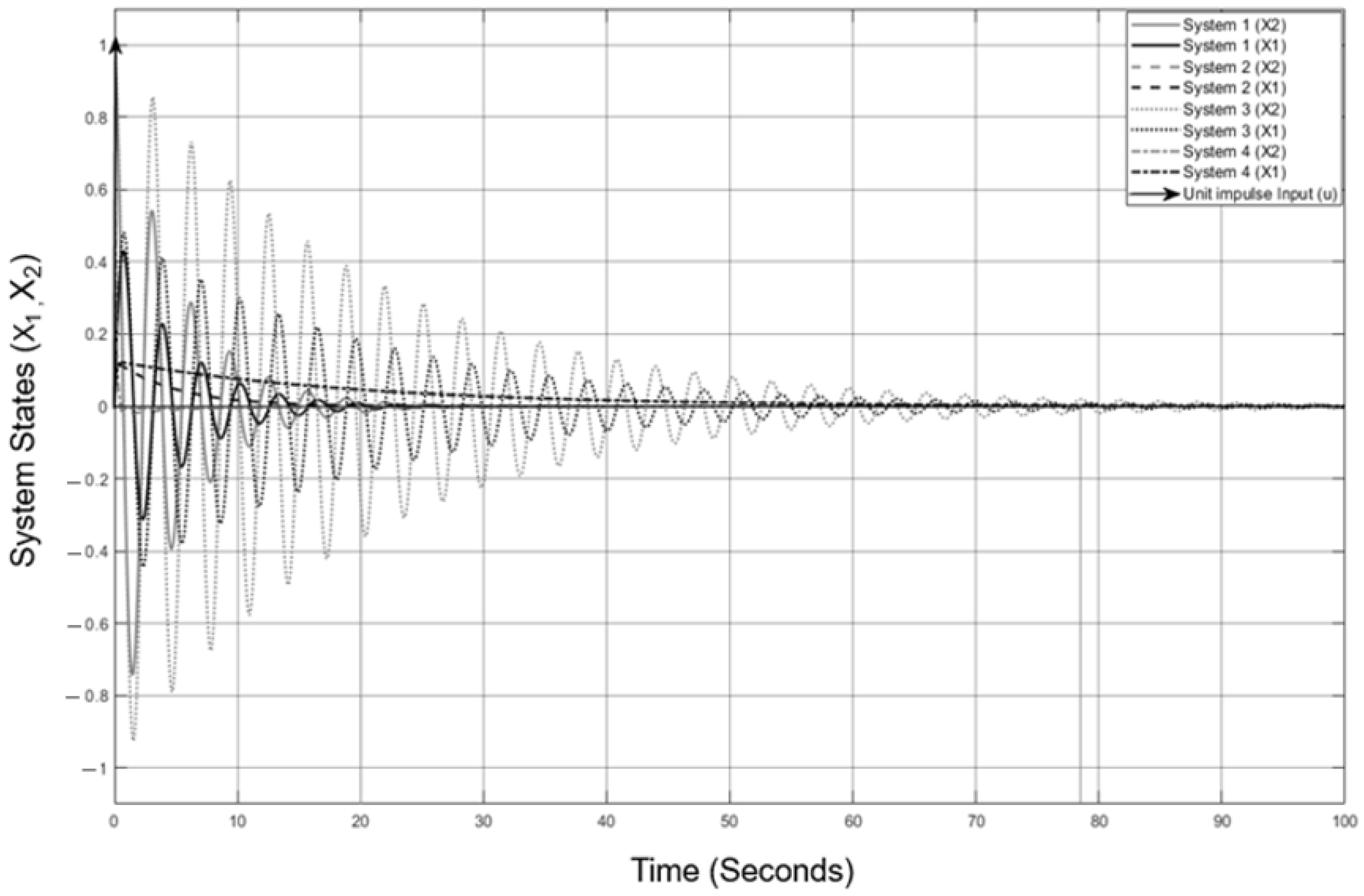
System 1: exponential oscillatory stability	$\left[\begin{array}{cc}-0.4& -4\\ 1& 0\end{array}\right]$	−0.2000 + 1.9900 i	−0.2000 + 1.9900 i	−0.20	20 s	$\mathrm{Underdamped} \mathrm{case} \zeta <1$
System 2: exponential monotonic stability	$\left[\begin{array}{cc}-8.4& -1.6\\ 1& 0\end{array}\right]$	−8.0000	−0.2000	−0.20	20 s	$\mathrm{Over} \mathrm{damped} \zeta >1$
System 3: exponential oscillatory stability	$\left[\begin{array}{cc}-0.1& -4\\ 1& 0\end{array}\right]$	−0.0500 + 1.9994 i	−0.0500 + 1.9994 i	−0.05	78 s	$\mathrm{Underdamped} \mathrm{case} \zeta <1$
System 5: exponential monotonic stability	$\left[\begin{array}{cc}-8.05& -0.4\\ 1& 0\end{array}\right]$	−8.0000	−0.0500	−0.05	78 s	$\mathrm{Over} \mathrm{damped} \zeta >1$

and Figure 10, two identical systems might have different amounts of passive control (damping) but as long as their dominant eigenvalues’ real parts are equal, the resulting settling times will be equal irrespective of their behavior (monotonic or oscillatory).

In the context of linear systems and a single domain of attraction, within a certain vicinity of the stable equilibrium, both passive control and rate of return to equilibrium increase until an optimum amount of resistance is reached (e.g., critical damping for second-order linear systems). Any further increase in passive control will negatively affect the settling time. Thus, engineering resilience is directly proportional to dynamic stability (within an open-loop setting with zero active control action) for a certain interval of passive control (e.g., critical damping) only. Beyond the interval of passive control, any added amount of passive control might curtail the system’s ability for innovation or might lock the system into domains with unproductive conditions such as economic recessions. The relationship between passive feedback and settling time, the two elements of engineering resilience, is demonstrated for two simple linear and nonlinear dynamic systems in

Table 6. Dynamic stability as a measure of engineering resilience for impulse input disturbance (δ(t)) (Case examples 1 and 2).

System	Case Example 1		Case Example 2
	Dynamic Stability (Settling Time)	Resistance to Perturbation as Indicator of Passive Control (c)	Dynamic Stability (Settling Time)	Resistance to Perturbation as Indicator of Passive Control (c)
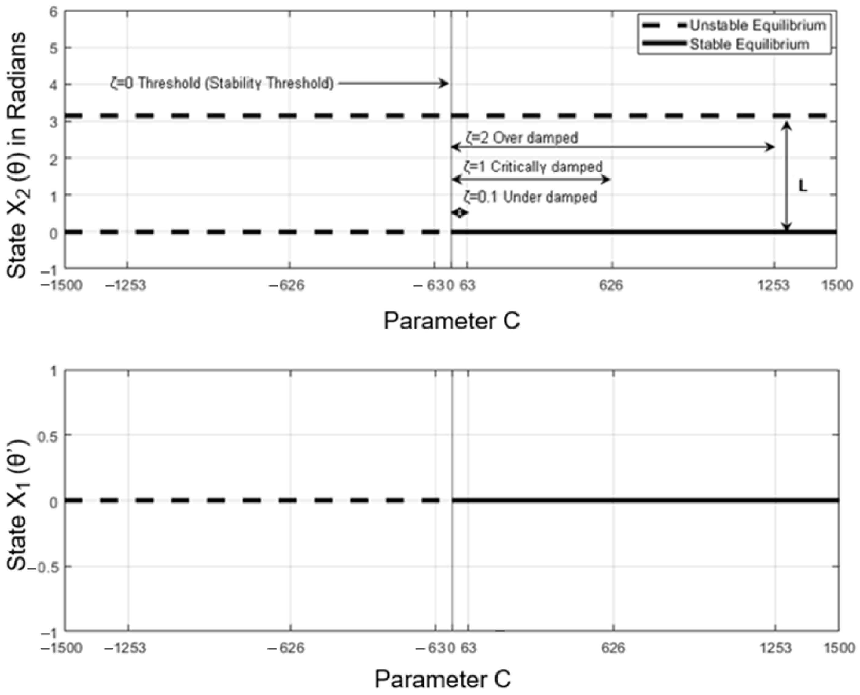
Marginal stable system $(\mathrm{not} \mathrm{damped} \zeta =0$)	Never	0	Never	0
$\mathrm{Exponential} \mathrm{stable} \mathrm{system} (\mathrm{underdamped} \zeta =0.1$)	20 s	0.4	17 s	63
$\mathrm{Exponential} \mathrm{monotonic} \mathrm{stable} \mathrm{system} (\mathrm{critically} \mathrm{damped} \zeta =1$)	3.5 s	1	3 s	626
$\mathrm{Exponential} \mathrm{monotonic} \mathrm{stable} \mathrm{system} (\mathrm{overdamped} \zeta =2$)	8 s	2	7 s	1253

and Figure 11 and Figure 12.

A good measure for engineering resilience can be considered as the volume of the system’s 3-dimenstional state portrait, where the two horizontal axes indicate the system state deviations under input disturbance (passive control indicator) while the vertical axis indicates the system settling time (system state rate of return to equilibrium). This combines both of the engineering resilience elements and the smaller the volume the larger the resilience becomes (Figure 13). For an equal value of settling time, monotonic exponential stability renders a slightly higher value of engineering resilience than that of oscillatory exponential stability given the slightly higher area of the system state trajectory around equilibrium of the former compared to the latter (Figure 10).

However, for linear systems the dynamic stability remains constant within the domain of attraction. In the context of nonlinear systems, the dynamic stability critically decreases (lengthy settling times) in the vicinity of unstable equilibrium (instability threshold), which results in smaller values of engineering resilience. Figure 14 depicts how the system state response critically slows down near the unstable equilibrium threshold ($x_1=6.264 \mathrm{o}\mathrm{r} x_2=3.14 \mathrm{R}\mathrm{a}\mathrm{d})$ as does the resistance to perturbation.

The ability of the system to return to its equilibrium state ceases once the passive feedback of the system reaches zero (open-loop system with zero active control) or, alternatively, when the system eigenvalues are on the imaginary axis of the complex plane. By crossing the zero limit (c = 0), which can referred to as a soft threshold, the system stable equilibrium state [0, 0] turns into an unstable one (Figure 15).

5.2. Resilience as System’s Form Return Ability

The ability of a dynamic system to respond to change by returning the system to a starting position or another suitable form can be a local or global phenomenon and is mostly discussed in the socio-ecological resilience category, where maintaining the system identity and/or avoiding critical thresholds are the main objectives. Critical thresholds in the system form can be divided into soft and hard thresholds, where the former is easy, and the latter is hard or impossible to reverse. The reversibility of the system form is a management action under the resilience scenario. It is thoroughly covered by the active feedback/control action under the modern stability concept, which also means that the active feedback action changes the system form and subsequently alters the system’s passive control measures that define open-loop dynamic stability (Figure 5). Since changes to the system form under the engineering resilience definition are limited and known (generally within a domain of attraction), the control law for the closed-loop system does not change and is labeled as a robust (active) control. For socio-ecological resilience on the other hand, which has a wide and unknown range of system changes, the control law is not constant and therefore is categorized as adaptive (active) control (Figure 5). Additionally, there is input disturbance of either an instantaneous (impulse input) or permanent (step input) nature that can flip the system state into another stability domain; this, along with the system’s passive control, are the two main elements that are crucial for measuring socio-ecological resilience.

In the context of linear systems and a single domain of attraction and global dynamic stability (Case example 1), there is no limit on the input disturbance that leads to instability. Although the system is theoretically a globally stable system, performance/specification requirements can be imposed to limit the system domain of equilibrium to a certain boundary, e.g., maximum story drift/displacement in Case example 1, which practically renders local stability. Therefore, socio-ecological resilience tilts toward engineering resilience, which is mostly about the passive control built into the system (

Table 7. Dynamic stability as a measure of engineering resilience for impulse input disturbance (δ(t)) (Case examples 1 and 2).

System	Engineering Resilience/Socio-Ecological Resilience (Case Example 1)			Socio-Ecological Resilience (Case Example 2)
	Dynamic Stability (Settling Time)	Resistance (R) to Perturbation—Indicator of Passive Control (c)	Maximum Input Disturbance That Can Flip the System State into Another Stable Domain	Resistance (R) to Perturbation—Indicator of Passive Control (c)	Maximum Input Disturbance That Can Flip the System State into Another Stable Domain
$\mathrm{Marginal} \mathrm{stable} \mathrm{system}—\mathrm{not} \mathrm{damped} \zeta =0$	Never	0	Infinite	0	9.81
$\mathrm{Exponential} \mathrm{stable} \mathrm{system}—\mathrm{underdamped} \zeta =0.1$	20 s	0.4	Infinite	63	9.81
$\mathrm{Exponential} \mathrm{monotonic} \mathrm{stable} \mathrm{system}—\mathrm{critically} \mathrm{damped} \zeta =1$	3.5 s	1	Infinite	626	9.81
$\mathrm{Exponential} \mathrm{monotonic} \mathrm{stable} \mathrm{system}—\mathrm{overdamped} \zeta =2$	8 s	2	Infinite	1253	9.81

). In the context of nonlinear systems with multiple domains of attraction, e.g., Case example 2, or more complex nonlinear systems with hard thresholds described by fold bifurcations, a higher value of input disturbance that can flip the system into another stability domain along with a higher amount of passive control measures indicate a high level of socio-ecological resilience (Table 7 and Figure 16).

Contrary to the simple nonlinear systems (Case example 2—Figure 17), for complex nonlinear dynamic systems the relationship between parameters affecting the system matrix A (or Jacobian) (dynamic stability and passive control) and those moving the equilibrium states (e.g., input or active control action) is an area for further exploration; since the subject parameters are often entangled and/or of a double-edged sword nature, there is increased complexity in the trade-offs between engineering resilience vs. socio-ecological resilience.

Bifurcation diagrams are useful tools from nonlinear dynamics and structural stability that can be utilized for nonlinear dynamic systems with single parameter changes and can help define hard and soft thresholds for socio-ecological resilience. For a single parameter system, changes can assess how far a critical threshold is located from the current equilibrium state, as well as to indicate whether a threshold that has been crossed is reversible (Figure 18) or irreversible (Figure 19), which corresponds to a soft and hard loss of resilience, respectively [58]. A hard loss of resilience is known as hysteresis (path dependence or path memory) or fold bifurcation in complex nonlinear systems and it shows that the system trajectory not only depends on the parameter value but also depends on which side the parameter value is approached (e.g., parameter R in the spruce budworm model—Figure 19). This occurs where there are the multiple domains of attraction [27].

When system resilience under passive control is not satisfactory, active control action (given that the system is controllable) is required to alter the system form by shifting the system eigenvalues to a desired location and adjusting the system behavior accordingly (Figure 20). For instance, the subject linear system given in Case example 1 is fully controllable, but its current behavior is oscillatory and not satisfactory. A full state active feedback tool can be used to bring the underdamped oscillatory state behavior to a critical damped monotonic behavior (or, in alternative scenarios, to speed up the system settling time or stabilize the system in the case of instability). This will mean shifting the system poles from the underdamped case (${\mathsf{\lambda }}_1=-0.2000+1.9900 \mathrm{i},{ \mathsf{\lambda }}_2=-0.2000-1.9900 \mathrm{i}) \mathrm{to}$ a critically damped one (${\mathsf{\lambda }}_1={\mathsf{\lambda }}_2=$ −2.000). The reference scale (r) is set to zero (zero input/equilibrium state) and instead, the disturbance input is introduced in the form of the initial condition of [20 0] (Figure 20). The control action bears a cost, which needs to be assessed versus the performance improvement it brings about.

6. Discussion and Conclusions

Both dynamic and structural stabilities are principally dependent on the system parameters where the former is about the rate of return to equilibrium and the latter is about the current equilibrium distance from a fold bifurcation point, which means staying in the same domain of equilibrium. Engineering resilience, which focuses on maintaining the system performance under limited and known types of perturbations, is therefore partially covered by the open-loop dynamic stability with zero active control. Dynamic stability without active control action can be seen as a static return rate to equilibrium through the utilization of the passive control system after the perturbation stimulus is removed. Moreover, if the system return behavior and return rate are not satisfactory, the control action is the only means of rectifying the unsatisfactory situation. On the other hand, socio-ecological resilience, which focuses on maintaining the system identity and avoiding critical thresholds, is partially covered by structural stability (distance to soft or hard thresholds) by keeping a static distance from equilibrium. Here, control action is needed to adjust that distance as per the perturbation value and type, which are often unknown and with large variability, and requires a closed-loop dynamic stability with adaptive control as an alternative for socio-ecological resilience. Additionally, control systems tools, such as state controllability, are potential directions for developing tools that can systematically describe the reversibility of equilibrium states in complex dynamic systems and the trade-offs between dynamic and structural stabilities. This study reveals that the two major categories of engineering resilience and extended ecological resilience are intrinsically the reinvention of a closed-loop system dynamic stability with different types of active feedback structures. Moreover, structural stability describes key aspects of social-ecological resilience—including critical thresholds where, under change, a system loses the ability to return to the starting form or move to another suitable form through active feedback mechanisms or direct management actions.

References

- Leine, R.I. The Historical Development of Classical Stability Concepts: Lagrange, Poisson and Lyapunov Stability. Nonlinear Dynamics 2010, 59, 173–182. [Google Scholar] [CrossRef]
- Hahn, W. Generalities. Die Grundlehren der mathematischen Wissenschaften. In Stability of Motion; Hahn, W., Ed.; Springer: Berlin, Heidelberg, 1967; pp. 1–8. ISBN 978-3-642-50085-5. [Google Scholar]
- Timoshenko, S.P.; Gere, J.M. Theory of Elastic Stability, 2nd ed.; Engineering Societies Monographs; McGraw-Hill: New York, NY, USA, 1961; ISBN 0-486-47207-8. [Google Scholar]
- Newell, K.M.; Corcos, D.M. Variability and Motor Control; Human Kinetics Publishers: Champaign, IL, USA, 1993; ISBN 0-87322-424-8. [Google Scholar]
- Odum, E.P. Fundamentals of Ecology; W.B. Saunders Company: Philadelphia, PA, USA, 1953. [Google Scholar]
- Justus, J. Complexity, Diversity, and Stability. In A Companion to the Philosophy of Biology; John Wiley & Sons, Ltd.: Chichester, UK, 2007; pp. 321–350. ISBN 978-0-470-69659-0. [Google Scholar]
- Grimm, V.; Wissel, C. Babel, or the Ecological Stability Discussions: An Inventory and Analysis of Terminology and a Guide for Avoiding Confusion. Oecologia 1997, 109, 323–334. [Google Scholar] [CrossRef] [PubMed]
- Yunes, M.A.M. Psicologia Positiva e Resiliência: O Foco No Indivíduo e Na Família. Psicol. Estud. 2003, 8, 75–84. [Google Scholar] [CrossRef]
- Sudmeier-Rieux, K. Resilience—an Emerging Paradigm of Danger or of Hope? Disaster Prev. Manag. 2014, 23, 67–80. [Google Scholar] [CrossRef]
- Holling, C.S. Resilience and Stability of Ecological Systems. Annu. Rev. Ecol. Syst. 1973, 4, 1–23. [Google Scholar] [CrossRef]
- Holling, C.S. Engineering Resilience versus Ecological Resilience. In Engineering within Ecological Constraints; Academy Press: Washington, DC, USA, 1996; p. 13. [Google Scholar]
- Bhamra, R.; Dani, S.; Burnard, K. Resilience: The Concept, a Literature Review and Future Directions. Int. J. Prod. Res. 2011, 49, 5375–5393. [Google Scholar] [CrossRef]
- Scopus. Scopus Database Search on Resilience vs. Stability Literature. 2022. Available online: https://www.scopus.com/search/form.uri?display=basic (accessed on 8 August 2022).
- Van Meerbeek, K.; Jucker, T.; Svenning, J.-C. Unifying the Concepts of Stability and Resilience in Ecology. J. Ecol. 2021, 109, 3114–3132. [Google Scholar] [CrossRef]
- Odum, E.P. Ecology and Our Endangered Life-Support Systems, 2nd ed.; Sinauer Associates: Sunderland, MA, USA, 1989; ISBN 0-87893-635-1. [Google Scholar]
- Seybold, C.A.; Herrick, J.E.; Brejda, J.J. Soil Resilience: A Fundamental Component of Soil Quality. Soil Sci. 1999, 164, 224–234. [Google Scholar] [CrossRef]
- Arnoldi, J.-F.; Loreau, M.; Haegeman, B. Resilience, Reactivity and Variability: A Mathematical Comparison of Ecological Stability Measures. J. Theor. Biol. 2016, 389, 47–59. [Google Scholar] [CrossRef]
- Dai, L.; Korolev, K.S.; Gore, J. Relation between Stability and Resilience Determines the Performance of Early Warning Signals under Different Environmental Drivers. Proc. Natl. Acad. Sci. USA 2015, 112, 10056–10061. [Google Scholar] [CrossRef]
- Mayar, K.; Carmichael, D.G.; Shen, X. Resilience and Systems—A Review. Sustainability 2022, 14, 8327. [Google Scholar] [CrossRef]
- Carmichael, D.G. The Conceptual Power of Control Systems Theory in Engineering Practice. Civ. Eng. Environ. Syst. 2013, 30, 231–242. [Google Scholar] [CrossRef]
- Carmichael, D.G. Structural Modelling and Optimization: A General Methodology for Engineering and Control; Ellis Horwood: Chichester, UK, 1981; ISBN 0-470-27114-0. [Google Scholar]
- De Oliveira, M.C. Fundamentals of Linear Control; Cambridge University Press: Cambridge, UK, 2017; ISBN 1-107-18752-4. [Google Scholar]
- Zayas, V.A.; Low, S.S.; Mahin, S.A. A Simple Pendulum Technique for Achieving Seismic Isolation. Earthq. Spectra 1990, 6, 317–333. [Google Scholar] [CrossRef]
- Dandy, G.; Walker, D.; Daniell, T.; Warner, R.; Foley, B. Planning and Design of Engineering Systems, 2nd ed.; CRC Press: London, UK, 2017; ISBN 1-138-03192-5. [Google Scholar]
- Kossiakoff, A.; Sweet, W.N. Systems Engineering: Principles and Practices, 2nd ed.; Wiley-Interscience: Hoboken, NJ, USA, 2011; ISBN 0-471-23443-5. [Google Scholar]
- Blanchard, B.S.; Fabrycky, W.J.; Fabrycky, W.J. Systems Engineering and Analysis; Prentice Hall: Englewood Cliffs, NJ, USA, 1990; Volume 4. [Google Scholar]
- Khalil, H.K.; Grizzle, J.W. Nonlinear Systems; Prentice Hall: Upper Saddle River, NJ, USA, 2002; Volume 3. [Google Scholar]
- DiStefano, J.J.; Stubberud, A.J.; Williams, I.J. Schaum’s Outline of Feedback and Control Systems, 3rd ed.; McGraw-Hill Professional: New York, NY, USA, 1997. [Google Scholar]
- Beisner, B.E.; Haydon, D.T.; Cuddington, K. Alternative Stable States in Ecology. Front. Ecol. Environ. 2003, 1, 376–382. [Google Scholar] [CrossRef]
- Meyer, K. A Mathematical Review of Resilience in Ecology. Nat. Resour. Model. 2016, 29, 339–352. [Google Scholar] [CrossRef]
- Chesi, G. Domain of Attraction: Analysis and Control via SOS Programming; Lecture Notes in Control and Information Sciences; Springer-Verlag: London, UK, 2011; ISBN 978-0-85729-958-1. [Google Scholar]
- Ahmed, N.U. Dynamic Systems and Control with Applications; World Scientific Publishing Company: Singapore, 2006; ISBN 981-310-682-4. [Google Scholar]
- Levine, W.S. The Control Handbook, 2nd ed.; CRC Press: Boca Raton, FL, USA, 2010. [Google Scholar]
- Cull, P. Global Stability of Population Models. Bull. Math. Biol. 1981, 43, 47–58. [Google Scholar] [CrossRef]
- Hinrichsen, D. Mathematical Systems Theory I: Modelling, State Space Analysis, Stability and Robustness; Texts in Applied Mathematics, 48; Springer: Berlin, Heidelberg, 2005; ISBN 978-3-540-26410-1. [Google Scholar]
- Chen, G. Stability of Nonlinear Systems. Encycl. RF Microw. Eng. 2004, 6, 4881–4896. [Google Scholar]
- Kapitaniak, T.; Thylwe, K.-E. Monotonic Stability. Chaos Solitons Fractals 1996, 7, 1411–1415. [Google Scholar] [CrossRef]
- Dorato, P. An Overview of Finite-Time Stability. In Current Trends in Nonlinear Systems and Control: In Honor of Petar Kokotović and Turi Nicosia; Menini, L., Zaccarian, L., Abdallah, C.T., Eds.; Systems and Control: Foundations & Applications; Birkhäuser: Boston, MA, USA, 2006; pp. 185–194. ISBN 978-0-8176-4470-3. [Google Scholar]
- Hong, Y.; Wang, J.; Xi, Z. Stabilization of Uncertain Chained Form Systems within Finite Settling Time. IEEE Trans. Autom. Control 2005, 50, 1379–1384. [Google Scholar] [CrossRef]
- Bhat, S.P.; Bernstein, D.S. Finite-Time Stability of Continuous Autonomous Systems. SIAM J. Control Optim. 2000, 38, 751–766. [Google Scholar] [CrossRef]
- Amato, F.; De Tommasi, G.; Pironti, A. Finite-Time Stability: An Input-Output Approach; John Wiley & Sons: Croydon, UK, 2018; ISBN 1-119-14052-8. [Google Scholar]
- Sontag, E.D. Input to State Stability: Basic Concepts and Results. In Nonlinear and Optimal Control Theory: Lectures given at the C.I.M.E. Summer School held in Cetraro, Italy 19–29 June 2004; Agrachev, A.A., Morse, A.S., Sontag, E.D., Sussmann, H.J., Utkin, V.I., Nistri, P., Stefani, G., Eds.; Lecture Notes in Mathematics; Springer: Berlin, Heidelberg, 2008; pp. 163–220. ISBN 978-3-540-77653-6. [Google Scholar]
- Dorf, R.C. Modern Control Systems; Pearson Prentice Hall: Upper Saddle River, NJ, USA, 2005. [Google Scholar]
- Carmichael, D.G. Incorporating Resilience through Adaptability and Flexibility. Civ. Eng. Environ. Syst. 2015, 32, 31–43. [Google Scholar] [CrossRef]
- Mascolo, I. Recent Developments in the Dynamic Stability of Elastic Structures. Front. Appl. Math. Stat. 2019, 5, 51. [Google Scholar] [CrossRef]
- Batabyal, A.A.; Beladi, H. The Stability of Stochastic Systems: The Case of Persistence and Resilience. Math. Comput. Model. 1999, 30, 27–34. [Google Scholar] [CrossRef]
- Vu, H.V.; Esfandiari, R.S. Dynamic Systems: Modelling and Analysis; McGraw-Hill Science, Engineering & Mathematics: New York, NY, USA, 1997; ISBN 0-07-021673-8. [Google Scholar]
- Bingham, J.T.; Ting, L.H. Stability Radius as a Method for Comparing the Dynamics of Neuromechanical Systems. IEEE Trans. Neural Syst. Rehabil. Eng. 2013, 21, 840–848. [Google Scholar] [CrossRef]
- Margalef, R. Diversity and Stability: A Practical Proposal and a Model of Interdependence. Brookhaven Symp. Biol. 1969, 22, 25–37. [Google Scholar] [PubMed]
- Murdoch, W.W. Population Regulation and Population Inertia. Ecology 1970, 51, 497–502. [Google Scholar] [CrossRef]
- Orians, G.H. Diversity, Stability and Maturity in Natural Ecosystems. In Unifying Concepts in Ecology: Report of the Plenary Sessions of the First International Congress of Ecology, The Hague, The Netherlands, 8–14 September 1974; van Dobben, W.H., Lowe-McConnell, R.H., Eds.; Springer Netherlands: Dordrecht, The Netherlands, 1975; pp. 139–150. ISBN 978-94-010-1954-5. [Google Scholar]
- Connell, J.H.; Sousa, W.P. On the Evidence Needed to Judge Ecological Stability or Persistence. Am. Nat. 1983, 121, 789–824. [Google Scholar] [CrossRef]
- Anderies, J.M. Embedding Built Environments in Social–Ecological Systems: Resilience-Based Design Principles. Build. Res. Inf. 2013, 42, 1–13. [Google Scholar] [CrossRef]
- Jen, E. Stable or Robust? What’s the Difference? Complexity 2003, 8, 12–18. [Google Scholar] [CrossRef]
- Kouvaritakis, B.; Owens, D.H.; Grimble, M.J. Sensitivity and Robustness in Control Systems Theory and Design. Available online: https://digital-library.theiet.org/content/journals/10.1049/ip-d.1982.0049 (accessed on 20 July 2022).
- Anderies, J.M.; Folke, C.; Walker, B.; Ostrom, E. Aligning Key Concepts for Global Change Policy: Robustness, Resilience, and Sustainability. Ecol. Soc. 2013, 18, 1–21. [Google Scholar] [CrossRef]
- Csete, M.E.; Doyle, J.C. Reverse Engineering of Biological Complexity. Science 2002, 295, 1664–1669. [Google Scholar] [CrossRef] [PubMed]
- Ludwig, D.; Walker, B.; Holling, C.S. Sustainability, Stability, and Resilience. Conserv. Ecol. 1997, 1, 1–21. [Google Scholar] [CrossRef]