Integration Method for Response History Analysis of Single-Degree-of-Freedom Systems with Negative Stiffness

Abstract

The present article deals with the mathematical investigation of a negative-stiffness ideal system that can be used in seismic isolation of civil engineering structures. Negative-stiffness systems can be used in the seismic isolation of structures, because in the case of a strong earthquake, they do not easily allow vibrations to develop. These negative-stiffness systems can be significantly more efficient than the usual seismic isolation systems, as they drastically reduce the vibrational amplitudes of structures, as well as eliminate the inertial seismic structure loadings. The mathematical investigation of a negative-stiffness ideal system provides documented answers about the effect of negative-stiffness systems in the seismic behavior of structures. First, the differential equation of motion of a single-degree-of-freedom oscillator (SDoF) is formulated, without classical damping, but with negative stiffness. Furthermore, the mathematical solution of the equation of motion is given, where it is proven that this solution does not describe a structure vibration. Furthermore, the seismic structure motion follows an exponential increase when the seismic ground excitation is purely sinusoidal. Finally, to calculate the real response of the negative-stiffness system, a suitable modification of the Newmark iterative numerical method is proposed.

1. Introduction

Civil structures always exhibit positive stiffness because the Bernoulli’s Technical Bending Theory, the concomitant Betti Principle, the Maxwell–Mohr propositions, and the Castigliano theorem are always valid. In each case, all civil engineering structures are conservative systems when nonconservative forces, such as the typical hysteretic ones [1], are neglected; consequently, their mechanical energy is always constant during the response. On the contrary, civil engineering structures equipped with nonlinear devices [2,3] are characterized by a mechanical energy that varies with time due to the work done by the nonconservative force, according to the modified work–energy theorem.

As a result, the flexibility matrix of a conservative system, calculated by the flexibility method, is always symmetric and positive definite. Similarly, the stiffness matrix, which is calculated using the stiffness method (or the use of Finite Elements) is also symmetric and positive definite. It is noted that in a positive definite matrix, all its diagonal terms are greater than zero and also the matrix determinant is positive.

The physical meaning of the positive definite stiffness is as follows: When a force is enforced on a single-degree-of-freedom system, then the point where the force is applied always moves along the same direction of the applied force. Similarly, when a torque is enforced on a structure, then the torque application point is always rotated with the same direction of the torque. In this way, the virtual work is always positive and defined as the internal product of the force and the induced displacement or the internal product of the torque and the induced rotation angle. Negative-stiffness systems are not ordinary load-bearing systems but, in fact, are motion transmission mechanisms, suitably connected to the structures. In general, a negative-stiffness system is defined as a single-degree-of-freedom (SDOF) system in which, when a displacement (equal to unit) is applied to the direction of its degree of freedom, the internal resistance force cannot develop, but further displacement develops. This phenomenon is equivalent to the development of an additional internal force (which has the same direction as the abovementioned displacement) of the structure, which causes an increase in the SDOF system’s displacement. In other words, a negative-stiffness system is not opposed to motion as would be the case with a regular-stiffness spring, but instead strengthens the displacement.

Negative-stiffness systems were introduced for the first time by Molyneaux [4], but without practical application in civil engineering structures, because, many times, these phenomena were instantaneous without the required structure stability. Moreover, Alabuzhev et al. [5] gave elements of comprehensive analytical derivations about the negative-stiffness system. Furthermore, Platus [6] published one of the first articles on the negative-stiffness concept using basic examples of civil engineering structures. In the above articles, the use of such systems is proposed for the purpose of isolating the motion along the horizontal and vertical structure direction. Furthermore, each negative-stiffness system with positive mass has an unstable solution (Inman [7], see Section 1.8). On the other hand, in recent years, various negative-stiffness mechanisms have been applied on civil engineering structures using these as seismic isolation systems. In addition, Carella et al. [8,9] investigated a three-spring system with very low (practically zero) stiffness (Quasi-Zero Stiffness—QZS), but it had the disadvantage that this worked only for a small range of displacements, while for larger displacements, the stiffness of the system had a positive value. Since then, considerable research has been carried out on the feasibility of the practical application of QZS mechanisms, as examined in the studies of Yang et al. [10] and Zhou et al. [11].

Moreover, various isolation systems including zero-stiffness mechanisms have been proposed, such as that of Yingli and Xu [12], who proposed the use of a dual QZS mechanism as a more effective element for vibration absorption. It is also noteworthy the arrangement presented by Xu et al. [13], where five stiffness springs were used to form the zero-stiffness mechanism. An arrangement with five springs was also proposed recently by Zhang et al. [14], where the springs were connected to establish a QZS vibration isolation system, in order to prevent various vibrations induced by underwater environment that cause problems on marine noise measuring equipment. Later, Nagarajaiah [15] proposed an innovative, adaptable negative-stiffness system, which aims to reduce the base seismic shear-force of the structure and, also, to reduce the large values of displacements/accelerations that develop under high seismic actions. Attary et al. [16], presented a rotation-based Adaptive Passive device (RBMAP), consisting of gears and arms, which, if installed at the location of the isolation bearings of a bridge, can significantly reduce the seismic shear forces on the bridge piers, as has been shown by suitable experimental research. Recently, a negative-stiffness system called KDamper was proposed by Antoniadis et al. [17] and Sapountzakis et al. [18] and incorporates an extra damping system called “the Tuned Mass Damper (TMD) system”. A key feature of this device is that it ensures constant negative stiffness for an important range of displacement amplitudes, thereby reducing the total stiffness of the isolated structure and achieving adequate seismic isolation (Nagarajaiah and Varadaraian [19]; Nagarajaiah and Sonmez [20]).

In another article, a damping system combined with a negative-stiffness system to achieve more effective seismic isolation was presented by Mofidian and Bardaweel [21]. Furthermore, Zhou et al. [22] examined the use of two axial-magnetized permanent magnetic rings, in the formation of a negative-stiffness system in combination with springs. Similarly, the concept of using magnets in forming a negative-stiffness system was given in an article by Hoque et al. [23], where the examined isolation device consists of magnets and springs, which connect a base with an intermediate mass and a seismic isolation table.

A redundant planar rotational parallel mechanism (RPRPM), consisting of two parallel linear elements, which are fixed to a vertical bar having a hinge in its center, was presented by Kanfkang and Hongzhou [24]. In this system, there are four springs, rigidly attached to the ends of the two bars, both of which are crosswise; thus, the mechanism develops negative stiffness. Another form of negative-stiffness system that consists of an axis of continuous rotation, which is eccentrically loaded, and having springs at their two ends, was presented by Abbasi et al. [25]. Moreover, it is worth noting that the negative-stiffness device presented by Li et al. [26] comprised a pre-compressed spring that moves on a curved block through a roller. This system can be applied to a bridge as a seismic isolator, and the experimental investigation showed a reduction in the seismic shear force at the base of the structure for the post-yielding state of seismic isolation bearings. It is noted that in the linear elastic region, the positive stiffness of a system is practically independent of the loading. On the contrary, in the case of negative stiffness, special loads are often required to produce negative stiffness, such as the P-Delta effects (Adam and Jager [27]). Lastly, in the very significant paper by Wang et al. [28], it referred to a study of multi-degree-of-freedom (MDOF) structures equipped with a negative-stiffness-amplifying damper in order to reduce the interstorey drifts.

However, despite the abovementioned articles with reference to the practical application of negative-stiffness mechanisms, such systems need further analytical and mathematical investigation, in order to examine their response (acceleration, velocity, and displacement) during seismic excitations.

In the present article, the differential equation of motion of a linear single-degree-of-freedom oscillator without damping, but with negative stiffness and positive mass, is presented. Then, through the solution of this equation of motion, it is mathematically indicated that the response of a negative-stiffness oscillator does not mean oscillation. Furthermore, the concept of the “equivalent negative potential energy” is produced, which confronts the kinetic energy. Thus, an important energy absorption is achieved, despite the fact that the theoretic oscillator does not possess classical damping. In addition, response displacements follow an exponential increase, even if the base seismic excitation is purely sinusoidal and it is compatible with Inman’s theory (1996) for the general case of negative-stiffness systems. In the present article, in order to avoid the unstable solution of a negative-stiffness system, we propose that the negative stiffness has to been interrupted after the maximum ground seismic displacement (or after a suitable relative displacement) using a secondary positive stiffness on the system. Subsequently, an appropriate modification of the Newmark [29] iterative numerical method is proposed to approximate the numerical response of the negative-stiffness system. Finally, an appropriate numerical example is presented to determine the response of a negative-stiffness system using the proposed modified Newmark numerical method, where it is proven numerically that this negative-stiffness system is conservative.

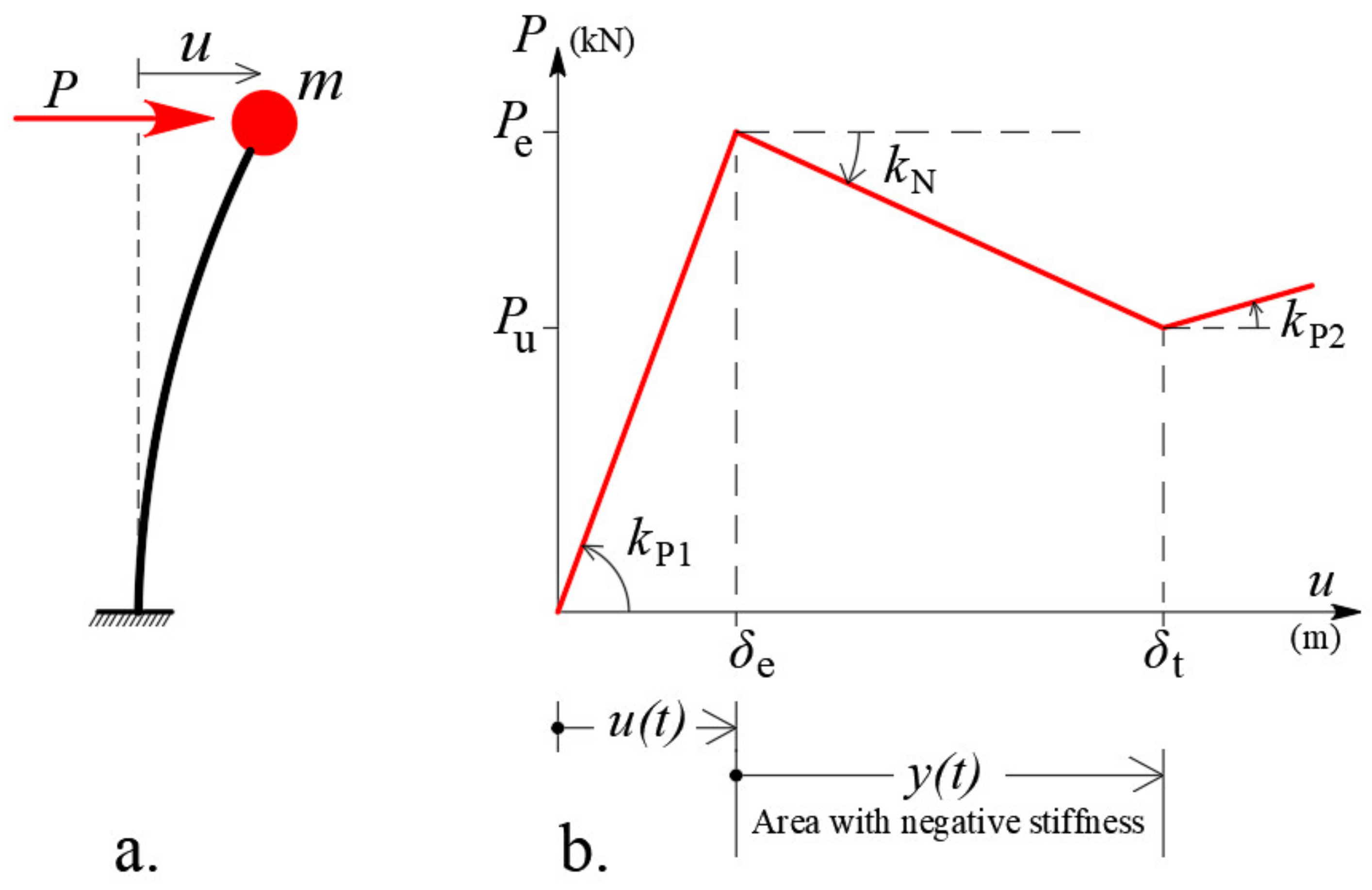
2. Analytical Investigation of a SDoF System with Positive and Negative Stiffness

Consider the ideal case of a single-degree-of-freedom oscillator of Figure 1a, which has mass m, zero damping, and is characterized by the following tri-linear law of response (Figure 1b). Initially, from the zero-displacement until yielding (in order to achieve negative stiffness) displacement ${\delta }_{enabled} \mathrm{or} {\delta }_e$, the SDOF oscillator possesses a positive stiffness $k_{P1}$ (i.e., $k_{P1}$ > 0), while for larger displacements (i.e., for $u>{\delta }_e$), the same oscillator possesses a negative stiffness $k_N$, where $k_N<0$. After the suitable relative displacement ${\delta }_u$, we consider an extra secondary positive stiffness $k_{P2}$ for safety reasons. The oscillation of the SDOF oscillator is examined in the following three phases:

-

Phase A (for response on the first branch, where stiffness is positive, equal to$k_{P1}$).

-

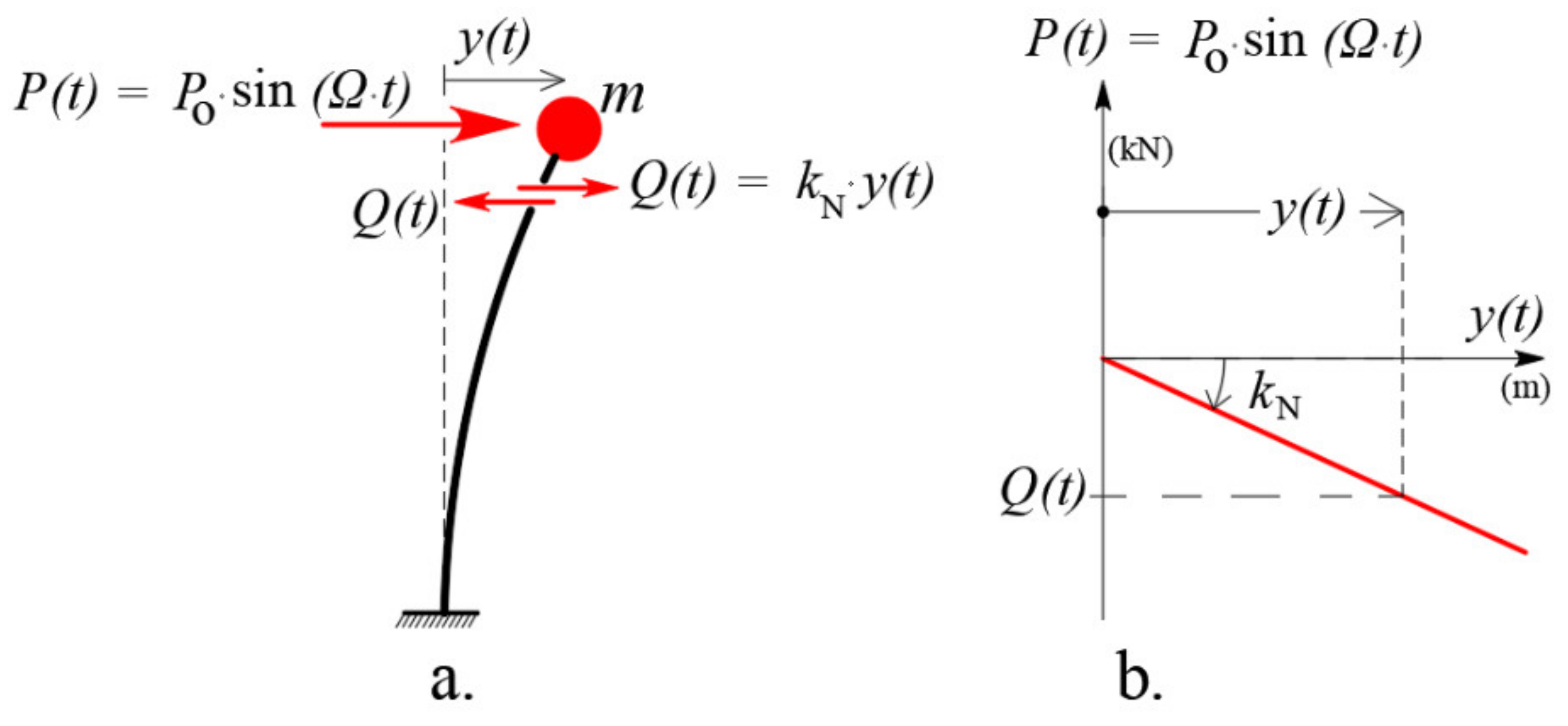
Phase B (for response on the second branch, where stiffness is negative, equal to $k_N$).

-

Phase C (for response on the third branch, where stiffness is positive, equal to $k_{P2}$).

2.1. Phase A: Mathematical Analysis of the Equation of Motion of the SDOF System for $u\left(t\right)\le {\delta }_e$

For the free oscillation of the SDOF oscillator on the first branch (i.e., when $u\left(t\right)\le {\delta }_{\mathrm{e}}$), where the oscillator possesses positive stiffness $k_{P1}$, the equation of motion for the free oscillation is:

$$m·\ddot{u}\left(t\right)+k_{p1}·u\left(t\right)=0$$

(1)

By dividing Equation (1) by mass m, we obtain:

$$\ddot{u}\left(t\right)+\frac{k_{p1}}{m}·u\left(t\right)=0$$

(2)

where quantity $k_{P1}/m$ is always positive because mass m and stiffness $k_{P1}$ are positive and, thus, ${\omega }_1^2=k_{P1}/m$. Quantity ${\omega }_1$ represents the cyclic frequency (in rad/s) of the oscillator. It is noted that the velocity (of mass) is defined as $\dot{u}\left(t\right)=du/dt$, while the acceleration of mass is defined as $\ddot{u}\left(t\right)=d^{2}u/d{t}^2$. In order to calculate the mechanical energy of this system for vibration on the first branch where $u(t$) $\le {\delta }_{\mathrm{e}}$, we multiply the members of Equation (1) by the differential displacement $du$ and, thus, the differential virtual work produced by the moving of the mass due to displacement $du$:

$$m·\ddot{u}\left(t\right)·du+k_{P1}·u\left(t\right)·du=0$$

(3)

By introducing the relation $du=\dot{u}\left(t\right)·dt$ into Equation (3), we obtain:

$$m·\ddot{u}\left(t\right)·\dot{u}\left(t\right)·dt+k_{P1}·u\left(t\right)·\dot{u}\left(t\right)·dt=0$$

(4)

Integrating Equation (4) with respect to time, from 0 to time $t_1$ where $u\left(t\right)={\delta }_e$ is true, shows that the change in the mechanical energy of the SDoF system (without damping), which possesses a positive stiffness $k_{P1}$, is zero.

$$\begin{gathered} {{\displaystyle \int }}_0^{t_1}m·\ddot{u}\left(t\right)·\dot{u}\left(t\right)·dt+{{\displaystyle \int }}_0^{t_1}{k}_{P1}·u\left(t\right)·\dot{u}\left(t\right)·dt=0 \Rightarrow \\ {{\displaystyle \int }}_0^{t_1}\frac{d}{dt}\left(\frac{1}{2}m·{\dot{u}}^2\left(t\right)\right)dt+{{\displaystyle \int }}_0^{t_1}\frac{d}{dt}\left(\frac{1}{2}{k}_{P1}·u^2\left(t\right)\right)dt=0 \Rightarrow \\ \left(\frac{1}{2}m·{\dot{u}}^2\left(t_1\right)-\frac{1}{2}m·{\dot{u}}^2\left(0\right)\right)+\left(\frac{1}{2}{k}_P·u^2\left(t_1\right)-\frac{1}{2}{k}_{P1}·u^2\left(0\right)\right)=0 \Rightarrow \\ \left(T\left(t_1\right)-T\left(0\right)\right)+\left(U\left(t_1\right)-U\left(0\right)\right)=0 \Rightarrow \\ T\left(t_1\right)+U\left(t_1\right)=T\left(0\right)+U\left(0\right) \end{gathered}$$

(5)

where $T\left(0\right)$ and $U\left(0\right)$ are the initial kinetic energy and initial potential energy of the undamped SDoF system, respectively; $T\left(t_1\right)$ and $U\left(t_1\right)$ are the kinetic energy and the potential energy of the undamped SDoF system, respectively, at time moment $t_1$, where $u\left(t_1\right)\le {\delta }_e$. Equation (5) shows that the total mechanical energy (sum of kinetic and potential energy) of the undamped SDOF system remains constant at any other time t until time $t_1$ (Chopra [30]). Equation (2) is also written as:

$${\omega }_1^2=-\frac{\ddot{u}\left(t\right)}{u\left(t\right)}$$

(6)

which indicates that at each time t ($0\le t\le t_1$), the asked displacement time-history $u\left(t\right)$ is always proportional to the second derivative of $\ddot{u}\left(t\right)$ in relation (6), as the first-order derivative does not exist. Moreover, the second derivative of the response displacement, namely the response acceleration time-history $\ddot{u}\left(t\right)$, is analogous with $-{\omega }_1^2$ concerning the response displacement time-history $u\left(t\right)$. Therefore, both the time functions $u\left(t\right)$ and $\ddot{u}\left(t\right)$ have to possess the same form of time function to simplify them, while the time function form must possess the special property to remain the same after two time-derivations. Out of all the different forms of time functions, the following two are those that have the above property:

$$u\left(t\right)=A·\sin {\omega }_{1}t$$

(7)

$$u\left(t\right)=A·e^{\lambda ·t}$$

(8)

where $A$ is a number representing the oscillation amplitude of the SDoF oscillator,$\lambda$ is a factor and $e=2.71828$... is the base of the natural logarithm, Equation (7) is a harmonic function, while Equation (8) is an exponential function. Equation (6) is directly verified by introducing Equation (7), which proves that the parameter ${\omega }_1$ is the cyclic frequency (in rad/s) of the SDoF oscillator. However, the solution of Equation (8) also verifies Equation (6) because the following equations are true:

$$\dot{u}\left(t\right)=A·\lambda ·e^{\lambda ·t}$$

(9)

$$\ddot{u}\left(t\right)=A·{\lambda }^2·e^{\lambda ·t}$$

(10)

By inserting Equations (8) and (10) into Equation (6), it is immediately given that:

$${\lambda }^2=-{\omega }_1^2$$

(11)

from which we obtain:

$$\lambda ={\omega }_{1}i$$

(12)

where $i=\sqrt{-1}$. Consequently, the solution of Equation (8) is written:

$$u\left(t\right)=A·e^{{\omega }_{1}t i}$$

(13)

However, using Euler’s complex exponential equation, we can write Equation (13) as follows:

$$u\left(t\right)=A·e^{{\omega }_{1}t i}=\left(A·\cos {\omega }_{1}t\right)+\left(A·\sin {\omega }_{1}t\right)i$$

(14)

The complex vector of the displacement $u\left(t\right)$ of Equation (14) can be represented at the complex plane (Gauss plane, Figure 2), where the real part expresses the natural phenomenon of harmonic oscillation with cyclic frequency ${\omega }_1$ (here identified as a solution of the harmonic function of Equation (7)), while the imaginary part is used to calculate the argument (i.e., the angle of the trigonometric numbers appearing in the solution), as well as to calculate the modulus of the complex number, which, in this case, is identified by the oscillation amplitude of the SDoF oscillator.

Indeed, the absolute modulus value $r$ of the complex number $u\left(t\right)$ in every time step t is:

$$r=\sqrt{{\left(A·\cos {\omega }_{1}t\right)}^2+{\left(A·\sin {\omega }_{1}t\right)}^2}=A$$

(15)

We observe that the complex solution of Equation (14) resulting from the exponential function of Equation (8) gives a more complete qualitative and numerical interpretation of the oscillation of the SDoF oscillator, which possesses positive stiffness $k_{P1}$.

2.2. Phase B: Mathematical Analysis of the SDoF System for $u\left(t\right)>{\delta }_e$

Consider that at time $t_1$, the displacement $u\left(t\right)$ of mass $m$ that reaches the enabled displacement ${\delta }_e$, namely $u\left(t\right)>{\delta }_e$ is valid; then, the oscillator is inserted into the post-elastic area (Figure 1b), where the negative stiffness $k_N$ occurs for each plastic displacement $y\left(t\right)>0$, where $t_1\le t$:

$$y\left(t\right)=u\left(t\right)-{\delta }_e$$

(16)

Then, the equation of motion, considering that $k_N$ is a pure negative parameter and, therefore, we use the absolute value of $k_N$, giving its negative sign—left from the absolute value, Equation (1)—is now written as:

$$m·\ddot{y}\left(t\right)-\left|k_N\right|·y\left(t\right)=0$$

(17)

and dividing by mass $m$, we obtain:

$$\ddot{y}\left(t\right)-\frac{\left|k_N\right|}{m}·y\left(t\right)=0$$

(18)

which is re-written as:

$$\ddot{y}\left(t\right)-{\omega }_2^2·y\left(t\right)=0$$

(19)

where ${\omega }_2^2=\left|k_N\right|/m$. Here, the parameter ${\omega }_2^{ }$ is a positive amount but does not represent an oscillation frequency. In order to calculate the mechanical energy of this mathematical ideal system for oscillation on the second branch only, where $y\left(t\right)>0$ is true, the two members of Equation (17) are multiplied by the differential displacement $dy$ and, thus, the differential virtual work produced due to movement of mass $m$ by$dy$:

$$m·\ddot{y}\left(t\right)·dy-\left|k_N\right|·y\left(t\right)·dy=0$$

(20)

By introducing the relation $dy=\dot{y}\left(t\right)·dt$ into Equation (20), we obtain:

$$m·\ddot{y}\left(t\right)·\dot{y}\left(t\right)·dt-\left|k_N\right|·y\left(t\right)·\dot{y}\left(t\right)·dt=0$$

(21)

Integrating Equation (21) with respect to time $t$, we obtain the mechanical energy of the SDoF oscillator, which possesses negative stiffness:

$$\begin{gathered} {{\displaystyle \int }}_{t_1}^{t}m·\ddot{y}\left(t\right)·\dot{y}\left(t\right)·dt-{{\displaystyle \int }}_{t_1}^t\left|k_N\right|·y\left(t\right)·\dot{y}\left(t\right)·dt=0 \Rightarrow \\ {{\displaystyle \int }}_{t_1}^t\frac{d}{dt}\left(\frac{1}{2}m·{\dot{y}}^2\left(t\right)\right)dt-{{\displaystyle \int }}_{t_1}^t\frac{d}{dt}\left(\frac{1}{2}\left|k_N\right|·y^2\left(t\right)\right)dt=0 \Rightarrow \\ \left(\frac{1}{2}m·{\dot{y}}^2\left(t\right)-\frac{1}{2}m·{\dot{y}}^2\left(t_1\right)\right)-\left(\frac{1}{2}\left|k_N\right|·y^2\left(t\right)-\frac{1}{2}\left|k_N\right|·y^2\left(t_1\right)\right)=0 \Rightarrow \\ \left(T\left(t\right)-T\left(t_1\right)\right)-\left(U\left(t\right)-U\left(t_1\right)\right)=0 \Rightarrow \\ T\left(t\right)+\left(-U\left(t\right)\right)=T\left(t_1\right)+\left(-U\left(t_1\right)\right) \end{gathered}$$

(22)

where $T\left(t_1\right)$ and $U\left(t_1\right)$ are the kinetic energy and potential energy, respectively, of the undamped SDoF system at time $t=t_1$, where the negative stiffness of the SDoF oscillator is activated and $T\left(t\right)$ and $U\left(t\right)$ are the kinetic energy and potential energy, respectively, of the undamped SDoF system that possesses negative stiffness for $y\left(t\right)>0$.

Equation (22) shows that potential energy acts competitively with the kinetic energy of the undamped SDoF system (which possesses negative stiffness), developing a new type of kinetic energy absorption (in other words, it brings an equivalent absorption), even though this SDoF system does not possess viscous and hysteretic damping. This new type of potential energy that causes the abovementioned absorption of kinetic energy is due to the negative sign of the potential energy relative to the positive sign of the kinetic energy, where Equation (22) shows that the two energies (kinetic and potential) act competitively with each other, causing an equivalent absorption of kinetic energy, while the damping is impossible in unstable systems (Inman [7]). The following numerical example of Section 3.2 shows that the mechanical energy is inclined to zero when stiffness is negative, which indicates that the mechanical energy is quasi-constant. Thus, a civil engineering structure with negative stiffness is a type of quasi-conservative system, because on the contrary case, it is well-known that each negative-stiffness system with positive mass has an unstable solution (Inman [7], see Section 1.8). For the solution of Equation (17), we have:

$${\omega }_2^2=\frac{\ddot{y}\left(t\right)}{y\left(t\right)}$$

(23)

which shows that at any time t (with $>t_1$), the asked response displacement time-history $y\left(t\right)$ is always proportional to the second derivative $\ddot{y}\left(t\right)$, as the first-order derivative is missing, having analogic factor ${\omega }_2^2$ (see at Equation (23)). Therefore, both the time functions $y\left(t\right)$ and $\ddot{y}\left(t\right)$ must have the same form of time function, to simplify them, while the form of time function must remain same, after two derivatives with reference to time. Of all the different forms of time functions, only the exponential function has the above property and can, therefore, be the solution as the harmonic function is not true now. Therefore:

$$y\left(t\right)=B·e^{\mu ·t}$$

(24)

where $B$ and $\mu$ are number coefficients. It is known that the following two equations are true:

$$\dot{y}\left(t\right)=B·\mu ·e^{\mu ·t}$$

(25)

$$\ddot{y}\left(t\right)={\rm B}·{\mu }^2·e^{\mu ·t}$$

(26)

By inserting Equations (26) and (24) into Equation (23), it is noticed that Equation (24) has to be:

$$\mu =\pm {\omega }_2$$

(27)

in order to be a solution. Therefore, the solution of Equation (24) is given by Equation (28) and shows that it is not a harmonic oscillation and the displacements $y\left(t\right)$ of the SDoF oscillator increase or decrease exponentially over time. Moreover, as it is shown in Equation (22), the inserted energy is absorbed:

$$y\left(t\right)=B·e^{\pm {\omega }_{2}t}$$

(28)

The above results: (a) the fact that there can be no oscillation in the negative-stiffness systems, because it leads to an exponential increase in displacements u(t); (b) the fact that the mechanical energy of the system is drastically reduced (due to competitive kinetic and potential energy action), allow the use of negative-stiffness systems for seismic isolation of structures (as it has been experimentally shown to work according to the references already mentioned), while simultaneously reducing (or zeroing practically) the mechanical energy of the system. Conversely, classical seismic isolation alters the fundamental period of the structure and drives it out of the resonance area, while negative-stiffness systems do not even allow the oscillation and nullify the mechanical energy of the system.

2.3. Phase C: Mathematical Analysis of the Equation of Motion of the SDOF System for ${\delta }_t\le u\left(t\right)$

For the free oscillation of the SDOF oscillator on the third branch (i.e., when the seismic target displacement is smaller by displacement $u\left(t\right)$, namely ${\delta }_{\mathrm{t}}\le u\left(t\right)$), where the oscillator possesses the secondary positive stiffness $k_{P2}$, the case is same with Phase A.

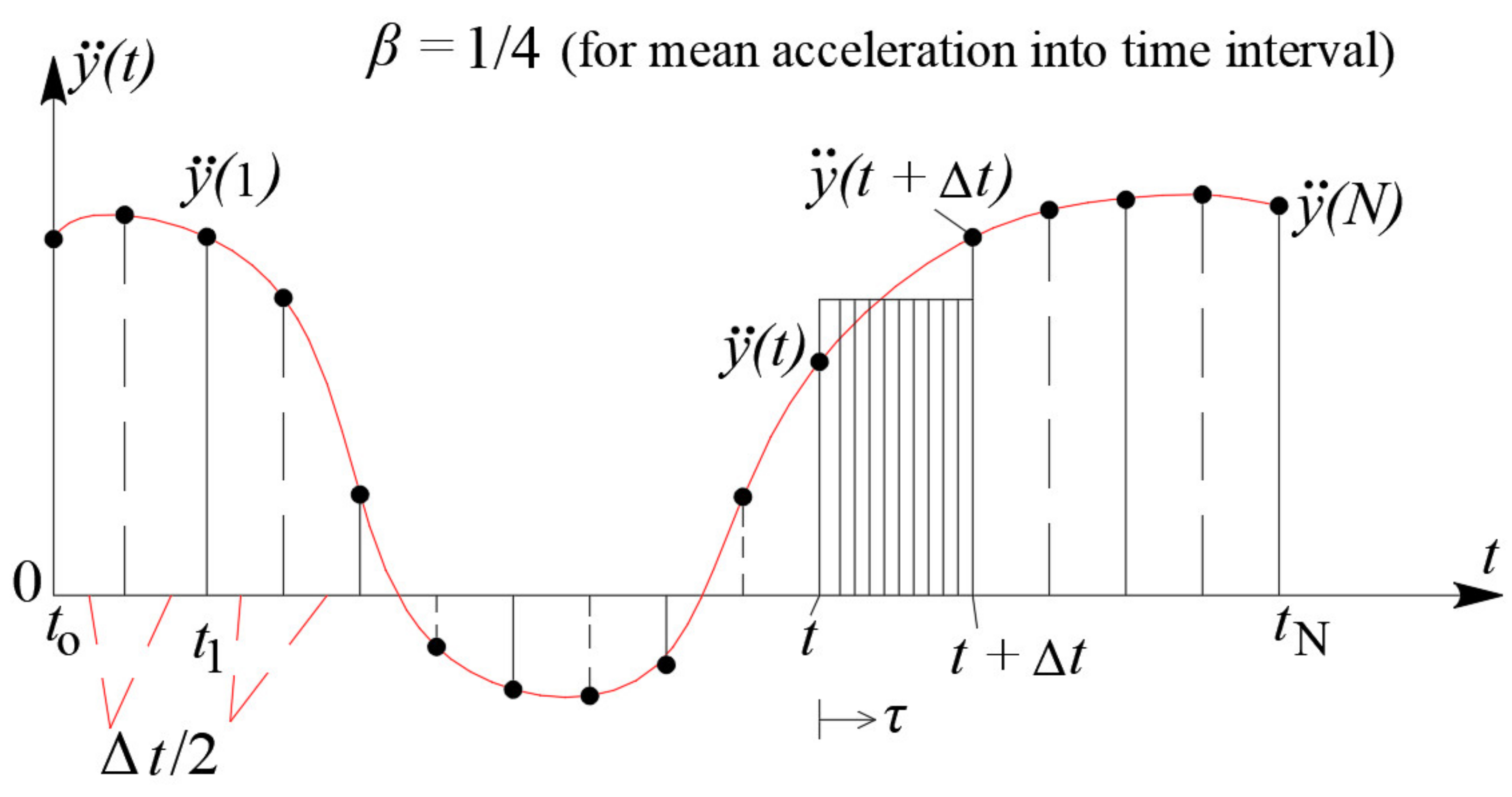
3. Adaptation of the Newmark Numerical Method to Solve the SDoF System with Negative Stiffness

There are several numerical methods available in the literature where dynamic response is calculated step by step [31]. The Newmark explicit time integration method is one of the oldest and most powerful methods used for dynamic analysis of structures. There are many advantages of this subfamily such as the possibility of unconditional stability for nonlinear systems and second-order accuracy, which leads to frequent use in structural dynamic analysis. Newmark’s method is simple and can be easily modified in ways that lead to new, more accurate methods for earthquake response analysis [32,33,34]. In the following paragraphs, it is described how Newmark’s Beta Method is adapted to calculate the response of an SDoF system with negative stiffness.

3.1. Analytical Formulation of the Adaptive Newmark Method to Solve SDoF System with Negative Stiffness

Consider the ideal case of an SDoF oscillator having only a negative stiffness $k_N$ and its mass (that is always positive) loaded with a dynamic sinusoidal loading $P\left(t\right)$ given by the following type (Figure 3):

$$P\left(t\right)=P_o·\sin \left(\Omega ·t\right)$$

(29)

We consider the initial/starting time (t = 0) at the moment where the above force is applied and, hence, the initial mass conditions (in terms of displacement, velocity, and acceleration) are equal to zero. For the formulation of the Newmark [26] numerical method, we consider the general case that the damping of the SDoF oscillator is c; then, the mass motion equation is given by Equation (30):

$$m·\ddot{y}\left(t\right)+c·\dot{y}\left(t\right)-\left|k_N\right|·y\left(t\right)=P\left(t\right)$$

(30)

We then adapt the Newmark [26] numerical method to the SDoF oscillator with negative stiffness for linear systems. Writing the motion equation at both ends $t+\mathsf{\Delta }t$ and t, of the differential time interval $\mathsf{\Delta }t$, we have:

$$m \ddot{y}\left(t+\mathsf{\Delta }t\right)+c \dot{y}\left(t+\mathsf{\Delta }t\right)-\left|k_N\right| y\left(t+\mathsf{\Delta }t\right)=P\left(t+\mathsf{\Delta }t\right)$$

(31)

$$m \ddot{y}\left(t\right)+c\dot{ y}\left(t\right)-\left|k_N\right| y\left(t\right)=P\left(t\right)$$

(32)

Subtracting the two above equations by members, the equation of motion over time $\mathsf{\Delta }t$ with zero initial conditions is given as:

$$m \mathsf{\Delta }\ddot{y}+c \mathsf{\Delta }\dot{y}-\left|k_N\right| \mathsf{\Delta }y=\mathsf{\Delta }P$$

(33)

where $\mathsf{\Delta }P=P\left(t+\mathsf{\Delta }t\right)-P\left(t\right)$. Note that Equation (33) is expressed as a function of differential differences $\mathsf{\Delta }y, \mathsf{\Delta }\dot{y}, \mathsf{\Delta }\ddot{y}$. We then form the differential differences $\mathsf{\Delta }y, \mathsf{\Delta }\dot{y}, \mathsf{\Delta }\ddot{y}$:

$$\mathsf{\Delta }y=y\left(t+\mathsf{\Delta }t\right)-y\left(t\right)$$

(34)

$$\mathsf{\Delta }\dot{y}=\dot{y}\left(t+\mathsf{\Delta }t\right)-\dot{y}\left(t\right)$$

(35)

$$\mathsf{\Delta }\ddot{y}=\ddot{y}\left(t+\mathsf{\Delta }t\right)-\ddot{y}\left(t\right)$$

(36)

The differential differences of Equations (34), (35), and (36) are a function of unknown values $y\left(t+\mathsf{\Delta }t\right),\dot{y}\left(t+\mathsf{\Delta }t\right), \ddot{y}\left(t+\mathsf{\Delta }t\right)$ of displacement, velocity, and acceleration, respectively, at time $t+\mathsf{\Delta }t$. The differential differences $\mathsf{\Delta }y, \mathsf{\Delta }\dot{y}, \mathsf{\Delta }\ddot{y}$ are then expressed by the known values $y\left(t\right), \dot{y}\left(t\right), \ddot{\mathrm{y}}\left(t\right)$ of displacement, velocity, and acceleration, respectively, at the preceding moment t by assuming how the response acceleration changes within the elementary time step $\mathsf{\Delta }t$. Thus, for various assumptions referring to the “acceleration distribution” (constant mean, linear, stepwise constant, parabolic, etc.) within $\mathsf{\Delta }t$, the “family of Newmark methods” is derived. In the present work, we used the assumption of a “constant mean acceleration” within the time intervals $\mathsf{\Delta }t$ (i.e., between two discrete time points), where the response acceleration of the oscillatory mass of a SDoF oscillator “is obtained constant and equal to half-sum of the two ends of each interval $\mathsf{\Delta }t$”. This is sometimes called “the average acceleration method” and it is unconditionally stable, meaning that the method will converge for all time increments. Therefore, in the period from t to $t+\mathsf{\Delta }t$, the response acceleration $\ddot{y}\left(t+\tau \right)$ is obtained from the half-sum expression:

$$\ddot{y}\left(t+\tau \right)=\frac{\ddot{y}\left(t\right)+\ddot{y}\left(t+\mathsf{\Delta }t\right)}{2} , 0\le \tau \le \mathsf{\Delta }t$$

(37)

Time τ denotes any time interval between times t and $t+\mathsf{\Delta }t$, according to Figure 4. By integrating Equation (37) with respect to τ, i.e., by calculating the shaded area of Figure 4 in time step τ, the following results:

$$\dot{y}\left(t+\tau \right)=\frac{\tau }{2}\cdot \left[\ddot{y}\left(t\right)+\ddot{y}\left(t+\tau \right)\right]+C_1$$

(38)

where $C_1$ is the integration constant, which has such a value that for $\tau =0$, the velocity is equal to that at the beginning of the time interval $\mathsf{\Delta }t$, i.e., $C_1=\dot{y}\left(t\right)$. Therefore, Equation (38) gives the final velocity value at the end of time step τ as:

$$\dot{y}\left(t+\tau \right)=\frac{\tau }{2}\cdot \left[\ddot{y}\left(t\right)+\ddot{y}\left(t+\tau \right)\right]+\dot{y}\left(t\right)$$

(39)

By performing a new integration, that is, a new calculation of the shading area of Figure 4 of Equation (39), the form of the displacement at the end of time step τ is given:

$$y\left(t+\tau \right)=\frac{{\tau }^2}{4}\cdot \left[\ddot{y}\left(t\right)+\ddot{y}\left(t+\tau \right)\right]+\tau \cdot \dot{y}\left(t\right)+C_2$$

(40)

where $C_2$ is the integration constant which, for $\tau =0$, must result in a displacement equal to that at the beginning of the time interval $\mathsf{\Delta }t$, i.e., $C_2=y\left(t\right)$. Therefore, Equation (40) gives the final value of the displacement at the end of time step τ:

$$y\left(t+\tau \right)=\frac{{\tau }^2}{4}\cdot \left[\ddot{y}\left(t\right)+\ddot{y}\left(t+\tau \right)\right]+\tau \cdot \dot{y}\left(t\right)+y\left(t\right)$$

(41)

Setting $\tau =\mathsf{\Delta }t$ at Equation (39) and Equation (41), we have:

$$\dot{y}\left(t+\mathsf{\Delta }t\right)=\frac{\mathsf{\Delta }t}{2}\cdot \left[\ddot{y}\left(t\right)+\ddot{y}\left(t+\mathsf{\Delta }t\right)\right]+\dot{y}\left(t\right)$$

(42)

$$y\left(t+\mathsf{\Delta }t\right)=\frac{{\left(\mathsf{\Delta }t\right)}^2}{4}\cdot \left[\ddot{y}\left(t\right)+\ddot{y}\left(t+\mathsf{\Delta }t\right)\right]+\mathsf{\Delta }t\cdot \dot{y}\left(t\right)+y\left(t\right)$$

(43)

By introducing the differential differences $\mathsf{\Delta }y, \mathsf{\Delta }\dot{y}, \mathsf{\Delta }\ddot{y}$ as given in Equations (34)–(36), respectively, into Equations (42) and (43), we obtain:

$$\dot{y}\left(t+\mathsf{\Delta }t\right)-\dot{y}\left(t\right)=\frac{\mathsf{\Delta }t}{2}\cdot \left[2·\ddot{y}\left(t\right)+\mathsf{\Delta }\ddot{y}\right]$$

(44)

$$y\left(t+\mathsf{\Delta }t\right)-y\left(t\right)=\frac{{\left(\mathsf{\Delta }t\right)}^2}{4}\cdot \left[2·\ddot{y}\left(t\right)+\mathsf{\Delta }\ddot{y}\right]+\mathsf{\Delta }t\cdot \dot{y}\left(t\right)$$

(45)

Solving Equation (45) with respect to $\mathsf{\Delta }\ddot{y}$ results in:

$$\mathsf{\Delta }\ddot{y}=\frac{4}{{\left(\mathsf{\Delta }t\right)}^2}\cdot \left[\mathsf{\Delta }y-\mathsf{\Delta }t\cdot \dot{y}\left(t\right)\right]-2·\ddot{y}\left(t\right)$$

(46)

and replacing Equation (46) by Equation (44), we have:

$$\mathsf{\Delta }\dot{y}=\frac{2·\mathsf{\Delta }y}{\mathsf{\Delta }t}-2·\ddot{y}\left(t\right)$$

(47)

Moreover, Equations (46) and (47) can be re-written as:

$$\mathsf{\Delta }\ddot{y}=\frac{1}{\beta \cdot {\left(\mathsf{\Delta }t\right)}^2}\cdot \mathsf{\Delta }y-\frac{1}{\beta \cdot \mathsf{\Delta }t}\cdot \dot{y}\left(t\right)-\frac{1}{2\beta }\cdot \ddot{y}\left(t\right)$$

(48)

where $\beta =0.25$, showing the mean acceleration into each time interval (Chopra, 2007) and

$$\mathsf{\Delta }\dot{y}=\frac{2\cdot \Delta y}{\Delta t}-2\cdot \dot{y}\left(t\right)$$

(49)

Therefore, Equations (48) and (49) express the differential differences in acceleration and velocity (i.e., $\mathsf{\Delta }\ddot{y}$ and $\mathsf{\Delta }\dot{y}$, respectively) as a function of time t. Thus, by inserting Equations (48) and (49) into Equation (33), we obtain:

$$\left[\frac{m}{\beta \cdot {\left(\mathsf{\Delta }t\right)}^2}+\frac{c}{2\beta \cdot \mathsf{\Delta }t}-\left|k_N\right|\right]\cdot \mathsf{\Delta }y=\mathsf{\Delta }p+\left[\frac{c}{2\beta }+\frac{m}{\beta \cdot \mathsf{\Delta }t}\right]\cdot \dot{y}\left(t\right)+\frac{m}{2\beta }\cdot \ddot{y}\left(t\right)$$

(50)

which is written in short form as:

$$\begin{gathered} {\widehat{k}}^{\ast }\cdot \mathsf{\Delta }y={\widehat{P}}^{\ast } \Rightarrow \\ \mathsf{\Delta }y=\frac{{\widehat{P}}^{\ast } }{{\widehat{k}}^{\ast }} \end{gathered}$$

(51)

where

$${\widehat{k}}^{\ast }=\frac{m}{\beta \cdot {\left(\mathsf{\Delta }t\right)}^2}+\frac{c}{2\beta \cdot \mathsf{\Delta }t}-\left|k_N\right|$$

${\widehat{k}}^{\ast }=$ the “equivalent stepping lateral stiffness” of the SDoF oscillator;

$${\widehat{P}}^{\ast }=\mathsf{\Delta }P+\left(\frac{c}{2\beta }+\frac{m}{\beta \cdot \mathsf{\Delta }t}\right)\cdot \dot{y}\left(t\right)+\frac{m}{2\beta }\cdot \ddot{y}\left(t\right)$$

${\widehat{P}}^{\ast }=$ the corresponding “equivalent stepping load” of the SDoF oscillator.

Equation (51) allows the calculation of the differential displacement $\mathsf{\Delta }y$ when the values of velocity $\dot{y}\left(t\right)$ and acceleration $\ddot{y}\left(t\right)$ are known at time t. Then, the differential differences in acceleration $\mathsf{\Delta }\ddot{y}$ and velocity $\mathsf{\Delta }\dot{y}$ are then calculated from Equations (48) and (49), respectively. Inverting Equations (34)–(36), we calculate the required values of displacement, velocity, and acceleration, respectively, at time $t+\mathsf{\Delta }t$:

$$y\left(t+\mathsf{\Delta }t\right)=y\left(t\right)+\mathsf{\Delta }y$$

(52)

$$\dot{y}\left(t+\mathsf{\Delta }t\right)=\dot{y}\left(t\right)+\mathsf{\Delta }\dot{y}$$

(53)

$$\ddot{y}\left(t+\mathsf{\Delta }t\right)=\ddot{y}\left(t\right)+\mathsf{\Delta }\ddot{y}$$

(54)

The above procedure accumulates rounding errors, clipping errors, and other errors. To eliminate these errors, the acceleration $\ddot{y}\left(t\right)$ must be obtained directly from the mass equation as follows:

$$\ddot{y}\left(t\right)=\frac{P\left(t\right)-c \dot{y}\left(t\right)+\left|k_N\right| y\left(t\right)}{m}$$

(55)

3.2. Algorithm of the Modified Newmark Method on a SDoF Negative-Stiffness System

From the abovementioned description of the Newmark method, the following calculation algorithm is summarized, with its steps listed in

Table 1. Algorithm of the Newmark-modified method for a SDoF system with negative stiffness (linear acceleration method (γ = 1/2, β = 1/4)).

Initial Calculations
1.1   $\ddot{y}\left(0\right)=\frac{P\left(0\right)-c \dot{y}\left(0\right)+\left|k_N\right| y\left(0\right)}{m}$
1.2 Time step selection Δt
1.3 $\alpha =\frac{1}{\beta \Delta t}m+\frac{\gamma }{\beta }c$$\mathrm{and} b=\frac{1}{2\beta }m+\mathsf{\Delta }t\left(\frac{\gamma }{2\beta }-1\right)$c
2. Calculations In Any Time Step i (Time t)
2.1 Determination of equivalent step load of the SDoF oscillator: $\hspace{1em}\hspace{1em}\hspace{1em}\hspace{1em}\hspace{1em}\hspace{1em}\hspace{1em}\hspace{1em}{\widehat{P}}^{\ast }=\mathsf{\Delta }P+\left(\frac{c}{2\beta }+\frac{m}{\beta \cdot \mathsf{\Delta }t}\right)\cdot \dot{y}\left(t\right)+\frac{m}{2\beta }\cdot \ddot{y}\left(t\right)$
$2.2 \mathrm{Determination} \mathrm{of} \mathrm{negative} \mathrm{stiffness} k_N$
$2.3 \mathrm{Determination} \mathrm{of} \mathrm{the} \mathrm{equivalent} \mathrm{stepping} \mathrm{lateral} \mathrm{stiffness} {\widehat{k}}_1^{*}$ of the SDoF oscillator: $\hspace{1em}\hspace{1em}\hspace{1em}\hspace{1em}\hspace{1em}\hspace{1em}\hspace{1em}\hspace{1em}{\widehat{k}}^{\ast }=\frac{m}{\beta \cdot {\left(\mathsf{\Delta }t\right)}^2}+\frac{c}{2\beta \cdot \mathsf{\Delta }t}-\left|k_N\right|$
2.4      $\mathrm{Solve} \mathrm{for} \Delta yi$
2.5 $\mathsf{\Delta }\dot{y}=\frac{2\cdot \Delta y}{\mathsf{\Delta }t}-2\cdot \dot{y}\left(t\right)$
2.6    $\mathsf{\Delta }\ddot{y}=\frac{1}{\beta \cdot {\left(\Delta t\right)}^2}\cdot \mathsf{\Delta }y-\frac{1}{\beta \cdot \mathsf{\Delta }t}\cdot \dot{y}\left(t\right)-\frac{1}{2\beta }\cdot \ddot{y}\left(t\right)$
2.7      $\mathsf{\Delta }yi=y\left(t+\mathsf{\Delta }t\right)-y\left(t\right)$ $\mathsf{\Delta }\dot{y}i=\dot{y}\left(t+\mathsf{\Delta }t\right)-\dot{y}\left(t\right)$ $\mathsf{\Delta }\ddot{y}$$\mathrm{i}=\ddot{y}\left(t+\mathsf{\Delta }t\right)-\ddot{y}\left(t\right)$
3. Repeat the procedure for the next time step. Replace i with i + 1 and repeat steps 2.1 to 2.7 for the next time step.

. To understand the abovementioned algorithm, we use a theoretical numerical example of a SDoF, a pure negative-stiffness oscillator with no damping (c = 0), which is loaded with a dynamic sinusoidal load of duration 5 s given by the following expression, Figure 5.

$$P\left(t\right)=P_o·\sin \left(\Omega ·t\right)=10·\sin \left(12.5663·t\right)$$

where $P_o=10 \mathrm{kN}$ and $\Omega =12.5663 \mathrm{rad}/\mathrm{s}$. The oscillator mass is $m=120 \mathrm{tons}$ and possesses a negative stiffness $k_N=-200 \mathrm{kN}/\mathrm{m}$. Τhe time step of analysis is selected to be $\mathsf{\Delta }t=0.02 \mathrm{s}$, while the three initial conditions of mass (displacement, velocity, and acceleration of the oscillator mass) are all zero. The following expressions are then defined at time step $\mathsf{\Delta }t=0.02 \mathrm{s}$:

$$\left(\frac{c}{2\beta }+\frac{m}{\beta \cdot \Delta t}\right)=\left(\frac{0}{2·0.25}+\frac{120}{0.25\cdot 0.02}\right)=\mathrm{24,000}$$

$$\frac{m}{2\beta }=\frac{120}{2·025}=240$$

(56)

$$\ddot{y}\left(0\right)=\frac{P\left(0\right)-c \dot{y}\left(0\right)+\left|k_N\right| y\left(0\right)}{m}=\frac{0-0·0.4+\left|-200\right| ·0}{120}=0$$

Then, the equivalent step loading ${\widehat{p}}_1^{\ast }$ is calculated at time $t_1=t_0+\mathsf{\Delta }t=0.00+0.02=0.02 \mathrm{s}$.

$$\begin{gathered} {\widehat{P}}_1^{\ast }=\mathsf{\Delta }P+\left(\frac{c}{2\beta }+\frac{m}{\beta \cdot \mathsf{\Delta }t}\right)\cdot \dot{y}\left(0\right)+\frac{m}{2\beta }\cdot \ddot{y}\left(0\right)= \\ =\left(2.486885\right)+\left(\mathrm{24,000}\right)\cdot \left(0.\right)+240\cdot \left(0.\right)=2.486885 \end{gathered}$$

The “equivalent stepping lateral stiffness” ${\widehat{k}}_1^{\ast }$ of the SDoF oscillator is then calculated.

$${\widehat{k}}_1^{\ast }=\frac{m}{\beta \cdot {\left(\mathsf{\Delta }t\right)}^2}+\frac{c}{2\beta \cdot \mathsf{\Delta }t}-\left|k_N\right|=\frac{120}{0.25\cdot {\left(0.02\right)}^2}+\frac{0}{2·0.25\cdot 0.02}-\left|-200\right|=\mathrm{1,199,800}$$

Therefore, the step increment $\mathsf{\Delta }{y}_1$ of the displacement in the first step is:

$$\mathsf{\Delta }{y}_1=\frac{{\widehat{P}}_1^{\ast } }{{\widehat{k}}_1^{\ast }}=\frac{2.486885}{1,199,800}=0.000002$$

The step increment $\mathsf{\Delta }{y}_1$ of the velocity in the first step is now calculated:

$$\mathsf{\Delta }{\dot{y}}_1=\frac{2\cdot \mathsf{\Delta }{y}_1}{\Delta t}-2\cdot \dot{y}\left(0\right)=\frac{2\cdot 0.000002}{0.02}-2\cdot 0.=0.000207$$

Therefore, the velocity $\dot{y}\left(0+0.02\right)$ and the displacement at the end of the time interval $\mathsf{\Delta }t$, i.e., at time $t_1=0.02 \mathrm{s}$, are:

$$\dot{y}\left(0+0.02\right)=\dot{y}\left(0\right)+\mathsf{\Delta }{\dot{y}}_1=0.+\left(0.000207\right)=0.000207$$

$$y\left(0+0.02\right)=y\left(0\right)+\mathsf{\Delta }{y}_1=0+0.000002=0.000002$$

Finally, the acceleration $\ddot{y}\left(0+0.02\right)$ at time $t_1=0.02 \mathrm{s}$ is given:

$$\begin{gathered} \ddot{y}\left(0+0.02\right)=\frac{P\left(0.02\right)-c·\dot{y}\left(0.02\right)+\left|k_N\right|·y\left(0.02\right)}{m}= \\ =\frac{2.486885-0·0.000207+\left|-200\right|·0.000002}{120}=0.020727 \end{gathered}$$

The abovementioned procedure is repeated for the next steps, while the results of the first four time steps are listed in

Table 2. Newmark Numerical Method for Linear Systems with Negative Stiffness.

t	$\mathit{P}\left(\mathit{t}\right)$	$\mathbf{\Delta }\mathit{P}$	$\ddot{\mathit{y}}\left(\mathit{t}\right)$	${\widehat{\mathit{P}}}^{\ast }$	${\widehat{\mathit{k}}}^{\ast }$	$\mathbf{\Delta }\mathit{y}$
0.00	0.0000		0.000000
0.02	2.486885	2.486885	0.020727	2.486885	1,199,800.0	0.000002
0.04	4.817512	2.330627	0.040166	12.279826	1,199,800.0	0.000010
0.06	6.845440	2.027928	0.057109	31.257021	1,199,800.0	0.000026
0.08	8.443249	1.597809	0.070505	58.239350	1,199,800.0	0.000049
0.10	….	….	….	…	….	…

and

Table 3. Newmark Numerical Method.

t	$\mathit{P}\left(\mathit{t}\right)$	$\mathbf{\Delta }\mathit{P}$	$\mathbf{\Delta }{\dot{\mathit{y}}}_{}$	$\dot{\mathit{y}}\left(\mathit{t}\right)$	$\mathit{y}\left(\mathit{t}\right)$
0.00	0.0000			0.00400	0.000000
0.02	2.486885	2.486885	−0.00012	0.00388	0.000079
0.04	4.817512	2.330627	−0.00012	0.003761	0.000155
0.06	6.845440	2.027928	−0.00012	0.003641	0.000229
0.08	8.443249	1.597809	−0.00012	0.003520	0.000301
0.10	….	….	….	….	…

. Figure 6, Figure 7 and Figure 8 show the response diagrams of the displacement, velocity, and acceleration of the oscillating mass of the undamped SDoF oscillator having negative stiffness, respectively. The same figures show the responses of the SDoF oscillator with different values of negative stiffness. We can see in Figure 6, Figure 7 and Figure 8 that in the case of such SDoF oscillators, all three response vectors (displacement, velocity, and acceleration) have the same sign and follow an exponential rate, without oscillation, and consequently, Equations (25), (26), and (28) are verified, even though the external dynamic loading is harmonious. Indeed, as the absolute value of negative stiffness increases, the more exponential the response results are, and as the negative stiffness approaches zero, a subtle oscillation begins to appear (see Figure 8 for $k_N=-100 \mathrm{kN}/\mathrm{m}$), which is due to a change in the sign of external potential, sinusoidal loading, and not to the SDoF system. This subtle mass oscillation decreases drastically with the increase in the absolute value of negative stiffness |$k_N$|. Figure 9 gives the numerical calculation of the kinetic energy, the potential energy, and the mechanical energy of the SDoF system with negative stiffness. We observe that the mechanical energy of the system, which is always defined as the sum of kinetic energy and potential energy, is now practically zero. This happens because the negative sign of stiffness is transferred to the potential energy and, therefore, the potential energy competes with the kinetic energy of the SDOF system. The zeroing of mechanical energy shows that the negative-stiffness system absorbs the mechanical energy, even though the examined oscillator has no classical damping.

4. Conclusions

The present paper aims to investigate through analytical methods the behavior of a theoretical, ideal SDoF oscillator with negative stiffness and positive mass, loaded with dynamic loading. The main conclusions of these procedures are listed below.

• The mathematical investigation of the motion of mas equation has shown that the mathematical equation of response for the theoretical SDoF negative-stiffness system is exponential, which leads to the conclusion that there can be no oscillation of negative-stiffness systems.
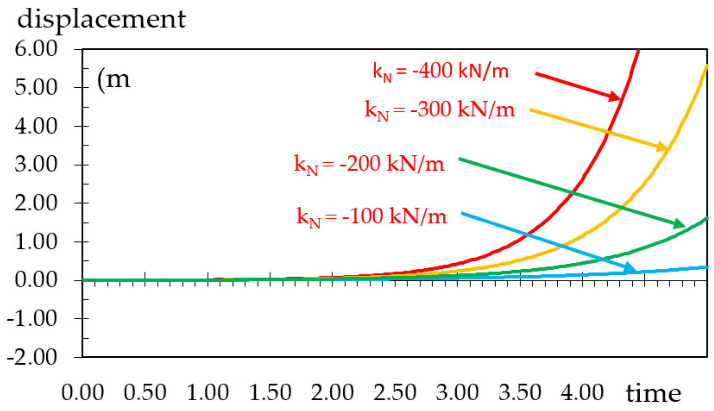
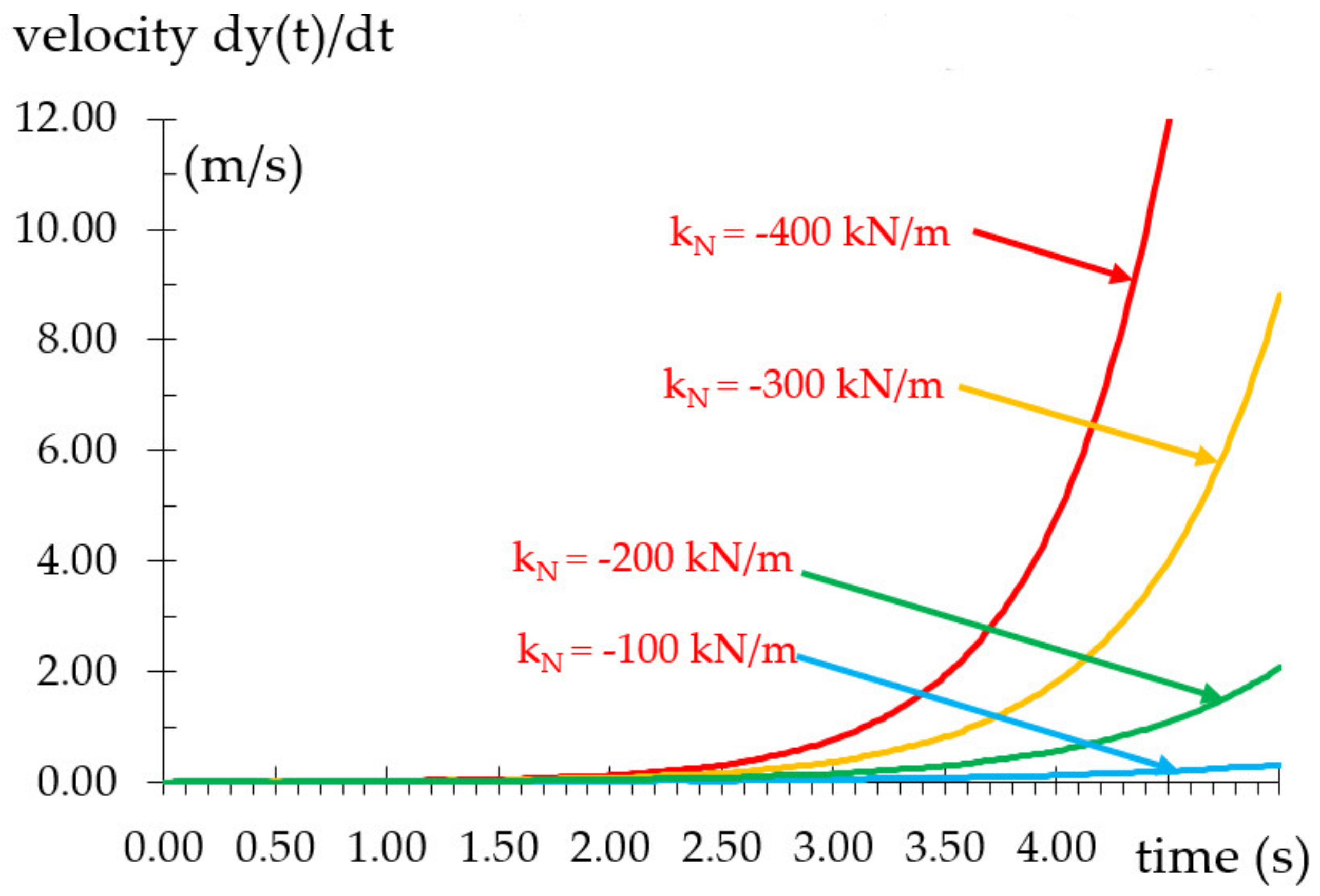
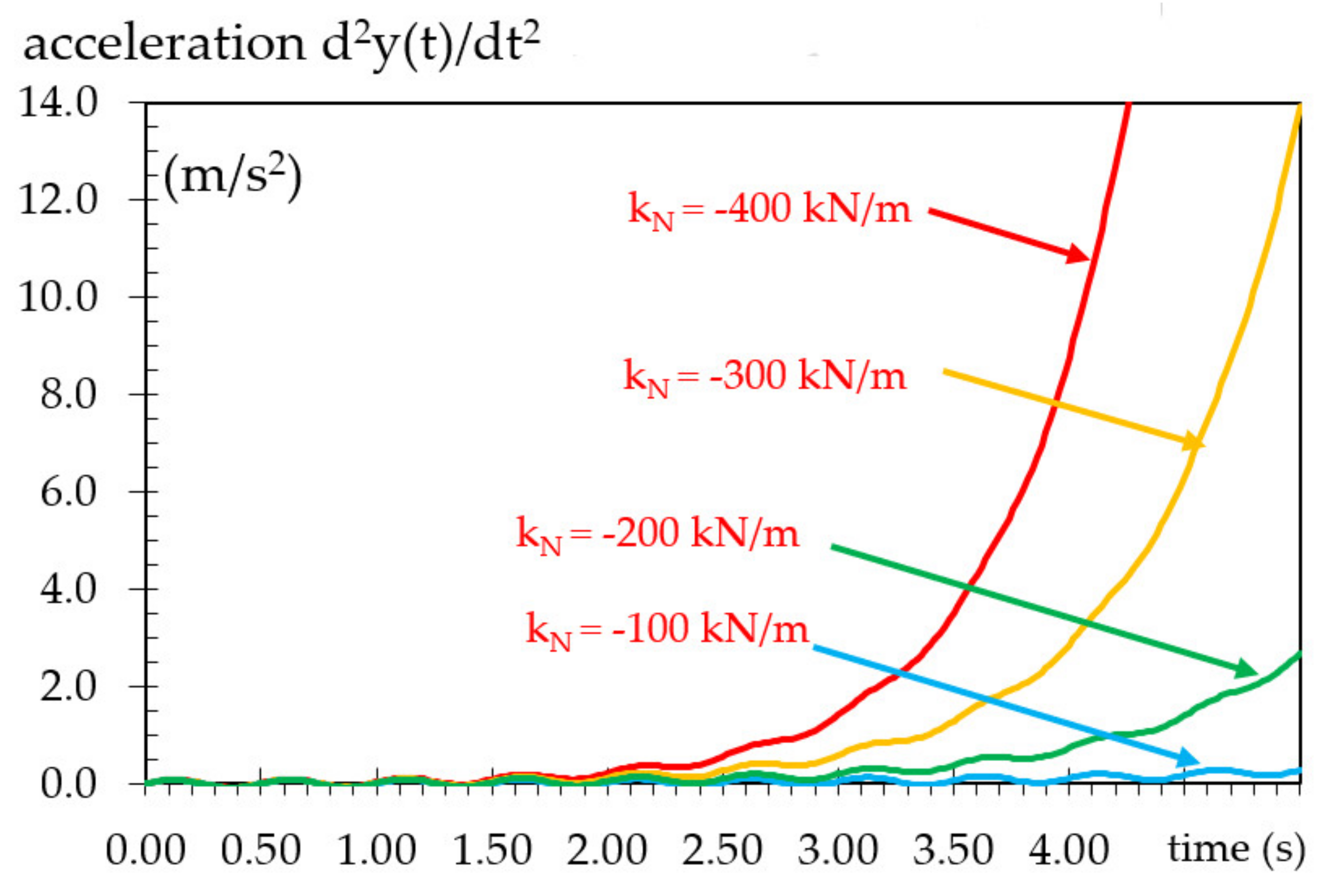
• The Newmark numerical method has been adapted with β = 0.25 and γ = 0.5 to calculate the response of such a system, and the influence of the magnitude of the absolute value of negative stiffness on the response results has been examined. As the absolute value of negative stiffness increases, the more exponential the response type is.
• Finally, it has been shown both analytically and numerically that in negative-stiffness systems, the mechanical energy of the system, which is always defined as the sum of kinetic energy and potential energy, is virtually zero, and this is due to the competitive action between kinetic energy and potential energy. The zeroing of the mechanical energy of a negative-stiffness SDoF shows an absorption of the kinetic energy, even though the examined SDoF oscillator is naturally undamped.
• Further investigation will include the examination of a negative-stiffness SDoF oscillator with viscous and hysteretic damping.

References

1. Vaiana, N.; Sessa, S.; Rosati, L. A generalized class of uniaxial rate-independent models for simulating asymmetric mechanical hysteresis phenomena. Mech. Syst. Signal Process. 2020, 146, 106984. [Google Scholar] [CrossRef]
2. Losanno, D.; Palumbo, F.; Calabrese, A.; Barrasso, T.; Vaiana, N. Preliminary Investigation of Aging Effects on Recycled Rubber Fiber Reinforced Bearings (RR-FRBs). J. Earthq. Eng. 2021, 26, 1–18. [Google Scholar] [CrossRef]
3. Vaiana, N.; Sessa, S.; Paradiso, M.; Marmo, F.; Rosati, L. An Efficient Computational Strategy for Nonlinear Time History Analysis of Seismically Base-Isolated Structures. In Lecture Notes in Mechanical Engineering, Proceedings of the XXIV AIMETA Conference, Rome, Italy, 15–19 September 2019; Springer: Berlin/Heidelberg, Germany, 2020; pp. 1340–1353. [Google Scholar] [CrossRef]
4. Molyneaux, W. Supports for Vibration Isolation; ARC/CP-322; Aer Res Council, G.: London, UK, 1957. [Google Scholar]
5. Alabuzhev, P.; Gritchin, A.; Kim, L.; Migirenko, G.; Chon, V.; Stepanov, P. Vibration Protecting and Measuring Systems with Quasi-Zero Stiffness. Applications of Vibration; Hemisphere Publishing Corp.: New York, NY, USA, 1989. [Google Scholar]
6. Platus, D.L. Negative-stiffness-mechanism vibration isolation systems. In Vibration Control in Microelectronics, Optics and Metrology; SPIE: Bellingham, WA, USA, 1991; Volume 1619, p. 44. [Google Scholar]
7. Inman, D.J.; Singh, R.C. Engineering Vibration; Prentice-Hall: Hoboken, NJ, USA, 1996; Volume 4. [Google Scholar]
8. Carella, A.; Brennan, M.; Waters, T. Static analysis of a passive vibration isolator with quasizero-stiffness characteristic. J. Sound Vib. 2007, 301, 678. [Google Scholar] [CrossRef]
9. Carrella, A.; Brennan, M.J.; Waters, T.P. Optimization of a quasi-zero-stiffness isolator. J. Mech. Sci. Technol. 2007, 21, 946–949. [Google Scholar] [CrossRef]
10. Yang, C.; Yuan, X.; Wu, J.; Yang, B. The research of passive vibration isolation system with broad frequency field. J. Vib. Control 2012, 19, 1348–1356. [Google Scholar] [CrossRef]
11. Zhou, J.; Wang, K.; Xu, D.; Ouyang, H.; Fu, Y. Vibration isolation in neonatal transport by using a quasi-zero-stiffness isolator. J. Vib. Control 2017, 24, 3278–3291. [Google Scholar] [CrossRef]
12. Yingli, L.; Xu, D. Force transmissibility of floating raft systems with quasi-zero-stiffness isolators. J. Vib. Control. 2017, 24, 3608. [Google Scholar] [CrossRef]
13. Xu, D.; Zhang, Y.; Zhou, J.; Lou, J. On the analytical and experimental assessment of the performance of a quasi-zero-stiffness isolator. J. Vib. Control 2013, 20, 2314–2325. [Google Scholar] [CrossRef]
14. Zhang, Y.; Mao, Y.; Wang, Z.; Gao, C. Nonlinear Low Frequency Response Research for a Vibration Isolator with Quasi-Zero Stiffness Characteristic. KSCE J. Civ. Eng. 2021, 25, 1849–1856. [Google Scholar] [CrossRef]
15. Nagarajaiah, S. Adaptive Negative Stiffness: A new structural modification approach for seismic protection. In Proceedings of the 5th World Conference on Structural Control and Monitoring, Tokyo, Japan, 12–14 July 2010. [Google Scholar]
16. Attary, N.; Symans, M.; Nagarajaiah, S. Development of a rotation-based negative stiffness device for seismic protection of structures. J. Vib. Control 2016, 23, 853–867. [Google Scholar] [CrossRef]
17. Antoniadis, I.; Kanarachos, S.; Gryllias, K.; Sapountzakis, E. KDamping: A stiffness based vibration absorption concept. J. Vib. Control. 2016, 24, 588. [Google Scholar] [CrossRef]
18. Sapountzakis, E.; Syrimi, P.; Pantazis, I.; Antoniadis, I. KDamper concept in seismic isolation of bridges with flexible piers. Eng. Struct. 2017, 153, 525–539. [Google Scholar] [CrossRef]
19. Nagarajaiah, S.; Varadarajan, N. Novel semi active variable stiffness tuned mass damper with real time tuning capacity. In Proceedings of the 13th Engineering Mechanics Conference; ASC: Reston, VA, USA, 2000. [Google Scholar]
20. Nagarajaiah, S.; Sonmez, E. Structures with semi active Variable Stiffness Single/Multiple Tuned Mass Dampers. J. Struct. Eng. 2007, 133, 67. [Google Scholar] [CrossRef]
21. Mofidian, S.; Bardaweel, H. Displacement transmissibility evaluation of vibration isolation system employing nonlinear-damping and nonlinear-stiffness elements. J. Vib. Control. 2017, 24, 4247. [Google Scholar] [CrossRef]
22. Zhou, Z.; Chen, S.; Xia, D.; He, J.; Zhang, P. The design of negative stiffness spring for precision vibration isolation using axially magnetized permanent magnet rings. J. Vib. Control 2019, 25, 2667–2677. [Google Scholar] [CrossRef]
23. Hoque, E.; Mizuno, T.; Ishino, Y.; Takasaki, M. A modified zero-power control and its application to vibration isolation system. J. Vib. Control 2011, 18, 1788–1797. [Google Scholar] [CrossRef]
24. Kangkang, L.; Hongzhou, J.; Jingfeng, H.; Hui, Z. Variable-stiffness decoupling of redundant planar rotational parallel mechanisms with crossed legs. J. Vib. Control 2018, 24, 5525–5533. [Google Scholar] [CrossRef]
25. Abbasi, A.; Khadem, S.; Bab, S. Vibration control of a continuous rotating shaft employing high-static low-dynamic stiffness isolators. J. Vib. Control 2016, 24, 760–783. [Google Scholar] [CrossRef]
26. Li, H.-N.; Sun, T.; Lai, Z.; Nagarajaiah, S. Effectiveness of Negative Stiffness System in the Benchmark Structural-Control Problem for Seismically Excited Highway Bridges. J. Bridg. Eng. 2018, 23, 04018001. [Google Scholar] [CrossRef]
27. Adam, C.; Jäger, C. Seismic Induced Global Collapse of Non-deteriorating Frame Structures. In Computational Methods in Earthquake Engineering; Springer: Berlin/Heidelberg, Germany, 2010; pp. 21–40. [Google Scholar] [CrossRef]
28. Wang, M.; Sun, F.; Nagarajaiah, S. Simplified optimal design of MDOF structures with negative stiffness amplifying dampers based on effective damping. Struct. Des. Tall Spéc. Build. 2019, 28, e1664. [Google Scholar] [CrossRef]
29. Newmark, N.M. A Method of Computation for Structural Dynamics. J. Eng. Mech. Div. 1959, 85, 67–94. [Google Scholar] [CrossRef]
30. Chopra, A.K. Dynamics of structures. In Mathematics and Archaeology; Prentice-hall International Series in Civil Engineering and Engineering Mechanics; Prentice-Hall: Hoboken, NJ, USA, 2007; pp. 164–183. [Google Scholar]
31. Vaiana, N.; Sessa, S.; Marmo, F.; Rosati, L. Nonlinear dynamic analysis of hysteretic mechanical systems by combining a novel rate-independent model and an explicit time integration method. Nonlinear Dyn. 2019, 98, 2879–2901. [Google Scholar] [CrossRef]
32. Hashamdar, H.; Ibrahim, Z.; Jameel, M. Finite element analysis of nonlinear structures with Newmark method. Int. J. Phys. Sci. 2011, 6, 1395–1403. [Google Scholar]
33. Alnahhal, W.; Aref, A. Numerical evaluation of dynamic response by using modified Newmark’s method. Jordan J. Civ. Eng. 2019, 13, 30–43. [Google Scholar]
34. Cui, Y.; Liu, A.; Xu, C.; Zheng, J. A Modified Newmark Method for Calculating Permanent Displacement of Seismic Slope considering Dynamic Critical Acceleration. Adv. Civ. Eng. 2019, 2019, 9782515. [Google Scholar] [CrossRef]
Figure 1. (a) SDOF oscillator; (b) positive and negative stiffness.
Buildings 12 01214 g001
Figure 2. The complex vector of displacement.
Buildings 12 01214 g002
Figure 3. (a) Harmonic loading of an ideal SDoF oscillator with negative stiffness; (b) negative stiffness.
Buildings 12 01214 g003
Figure 4. The change in acceleration between time t and t + Δ t (β = 0.25 for mean acceleration into each time interval, Chopra [30]).
Buildings 12 01214 g004
Figure 5. Graph of sinusoidal loading.
Buildings 12 01214 g005
Figure 6. Response displacements of SDoF oscillators with different values of negative stiffness.
Buildings 12 01214 g006
Figure 7. Response velocities of SDoF oscillators with different values of negative stiffness.
Buildings 12 01214 g007
Figure 8. Response accelerations of SDoF oscillators with different values of negative stiffness.
Buildings 12 01214 g008
Figure 9. Potential energy competes with kinetic energy resulting in the elimination of the mechanical energy of the SDOF system with negative stiffness.
Buildings 12 01214 g009