Comparative Analysis of Mechanical Performance of Flat Slabs with Reverse and Conventional Column Caps

Abstract

Compared with the conventional column caps, the reverse column caps that are used for slab-column joint of basement roof can improve the clearance of the basement while ensuring structural safety, and they are hidden in the covering soil without affecting the appearance and use of upper surface of flat slabs. In this paper, four finite element models, which are loaded by column-end displacement-control mechanism, are established. These models are used to investigate the mechanical performance of slab-column joint for flat slabs with reverse and conventional column caps. The obtained numerical results were thoroughly analysed, indicating that the load-carrying capacity performances of flat slabs with conventional column caps are much higher than their counterparts with reverse column caps, but flat slabs with conventional column caps possess lower mechanical ductility. Moreover, the reverse column caps were found to exhibit a severe damage at ultimate load; therefore, transverse stirrups were distributed into the reverse and conventional column caps for the purpose of comparison. The comparison results revealed that the ultimate load of the slab-column joints with reverse column cap can be increased by 2.4% by arranging transverse stirrups in column cap, but the ductility is decreased by 13.4%. For the slab-column joints with conventional column cap, the ultimate load is decreased by 10.0% and the ductility is decreased by 1.6% when transverse stirrups are arranged in column cap. Therefore, arrangement of transverse stirrups in column cap should be determined based on the actual situation in the flat slab system with reverse column cap, and it is not recommended to arrange transverse stirrups in column cap in the flat slab system with conventional column cap.

1. Introduction

Compared to the conventional beam-slab system, the flat slab requires less formwork in construction and can effectively reduce the overall height of the structure. Moreover, it gives a better appearance and provides a larger use of space. Therefore, flat slabs are commonly used in basement roof systems, in order to enlarge the basement clearance, facilitate the pipeline work and reduce the construction cost. In recent years, flat slabs have been increasingly adopted for the construction of large basement structures in China. As required by the municipal and planning departments, the basement roof needs to carry a 1–2 m deep layer of covering soil. In order to reduce the amount of covering soil and obtain an aesthetic basement space, new flat slabs with reverse column caps were proposed, resulting in flat slab bottoms and a larger basement space. Flat slabs may collapse due to the overweight of construction material piling or covering soil. The reverse column cap may impede transport vehicles, which can thus limit the occurrence of such situations to a certain extent. However, this new structural system has not been broadly used in engineering practices, due to the lack of sufficient research investigations and reliable design provisions [1].

The reinforced concrete flat slabs generally fail by punching shear failure, which can be attributed to the high shear stresses in the slab-column joint regions. Extensive testing, finite element (FE) modelling and analytical studies have been carried out to investigate this brittle failure. Several researchers [2,3,4,5,6] performed experimental investigations and proposed empirical equations based on the experimental observations, which have contributed to the development of the existing design codes [7,8]. On the basis of the empirical equations, scholars [9,10] investigated the effect of concrete strength on the load-carrying capacity of flat slabs and highlighted that high strength concrete can enhance the slab capacity. Genikomsou and Polak [11], Balomenos et al. [12], Wosatko et al. [13] and Alam et al. [14] performed FE modelling of reinforced concrete slabs and compared the FE models against the experiments, in order to investigate the effects of concrete stress–strain response and flexural reinforcements on the load-carrying capacity of flat slabs. Elsamak and Sabry [15] performed numerical simulations, highlighting that the load-carrying capacity and punching resistance of the flat slabs can be enhanced by increasing the slab thickness and bending reinforcements, but the failure mode remains the brittle punching shear failure. The influence of in-slab openings on the structural performance of flat slabs was examined by Yooprasertchai et al. [16], Hussain et al. [17] and Mostofinejad et al. [18]. Based on the existing database, Wu et al. [19] developed models to compare the existing data codes and revised the shear resistance equations for slab-column joints without punching reinforcements. Ma [20] explored the behavior of aged reinforced concrete columns under high sustained concentric and eccentric loads. Lin and Lin [21] carried out research on the moment distribution in the conventional column caps with different spans and cap widths, with the results revealing the shortcomings of the commonly used empirical coefficient method when applied to the conventional column caps; a new set of empirical coefficients was then proposed for the structural analysis of conventional column caps. Gong and Lu [22] compared the performance of the reverse and conventional column caps, highlighting that the reverse column caps are superior to their conventional counterparts in terms of interior space use.

In summary, the form of column cap and the stirrup of column cap in slab-column joints have not received much attention. In this paper, a numerical modelling investigation was performed to compare the load-carrying capacity and ductility performance of slab-column joints for flat slabs with reverse and conventional column caps, underpinned by an engineering practice. The relative positions of column caps and cap transverse stirrups were considered in the numerical modelling investigation. The obtained results can be used to provide references for the engineering design of flat slabs.

2. FE Modelling

This paper investigated the mechanical performance of slab-column joints by means of FE software Abaqus. Therefore, it is important to select a proper FE modelling method, which is critical in terms of computational efficiency and accuracy.

2.1. Selection of Solver

The core of Abaqus FE analysis software [23] is its solver module, which has two of the most commonly used solvers: Abaqus/Standard (implicit solver) and Abaqus/Explicit (explicit solver). Abaqus/Standard is a general-purpose FE analysis module and the most commonly used solver. It is often utilised to analyse static-state and quasi-static state problems, such as static-state analysis, steady-state problem analysis, thermo-mechanical coupling problem analysis and so on, including many non-structural problems. Abaqus/Explicit is often used to analyse transient state problems, such as short-term impact and collision, namely, a short-term process is simulated. This paper uses the static-state analysis in ABAQUS/Standard.

2.2. Element Type and Contact Settings

Abaqus provides a wide range of elements for users. There are five most commonly used element families, comprising solid elements, beam elements, shell elements, truss elements and rigid body elements. According to the slab-column joint type, concrete was simulated by using an 8-node hexahedral reduced integration element (C3D8R) to prevent the shear locking effect [23]; reinforcement was modelled by using a 2-node linear truss element (T3D2). Solid elements only need to define section properties to assign material properties to elements.

Regarding the FE modelling process, the key principle is to precisely simulate the practical situations and meanwhile ensure the computational accuracy and efficiency. The commonly used contact relationships include binding constraints, rigid body constraints, coupling constraints, embedded constraints and so on. For the FE modelling of cast-in-situ concrete slab-column joints, binding constraints were adopted for the contact between concrete components. Reference [24] proposed that the influence of bond slip on the load-carrying capacity of reinforced concrete structures could be neglected, so the embedded constraints were utilised for the contact between steel bars and concrete, which means the reinforcement model was completely embedded into the concrete model.

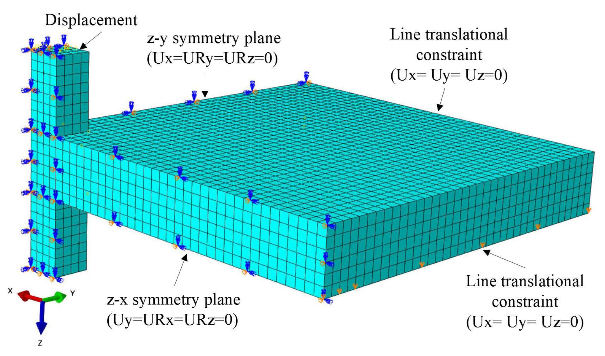
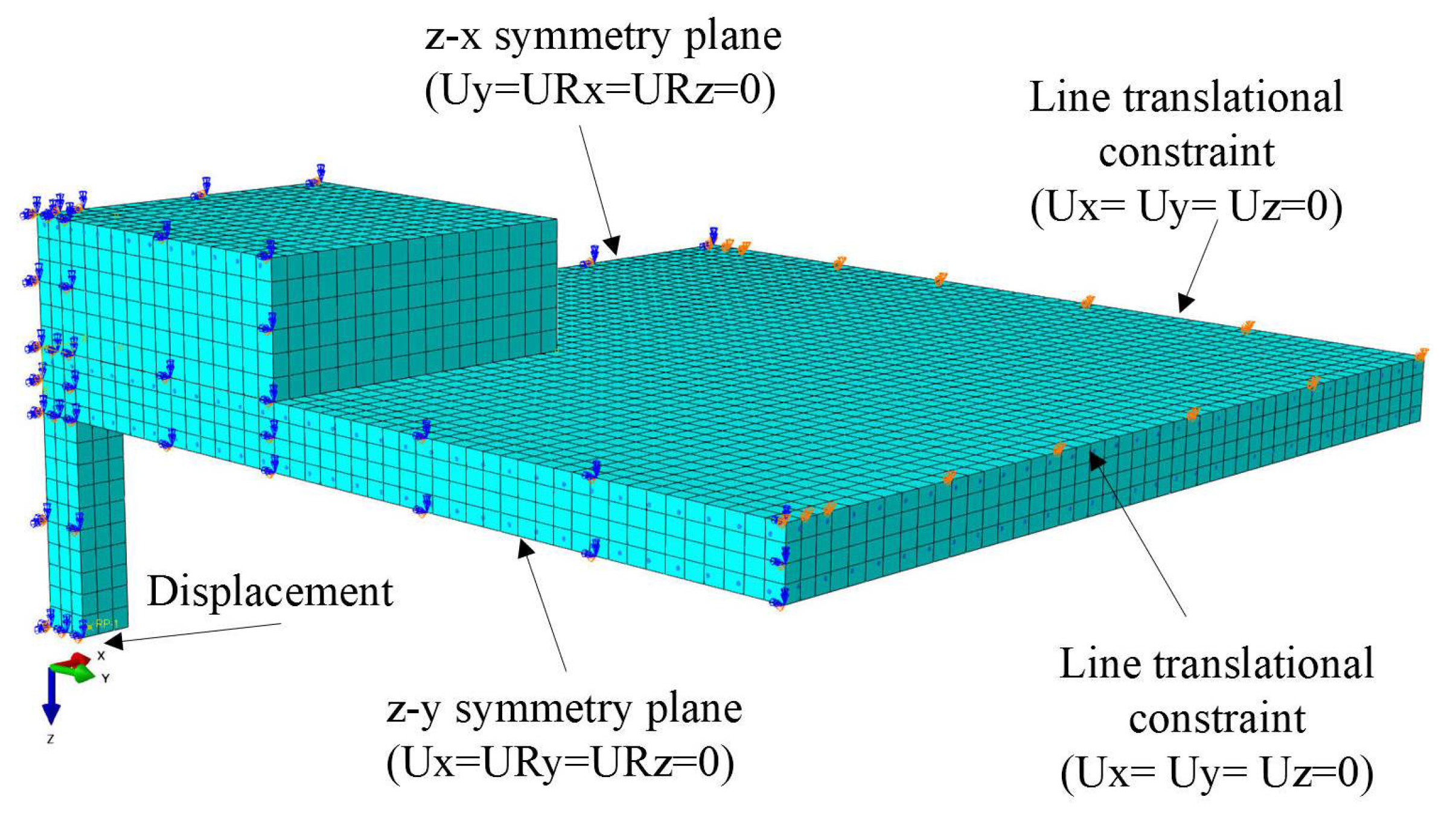
2.3. Loading Schemes and Boundary Conditions

Since the solid element C3D8R was used to simulate concrete in this paper, when applying loads or defining displacements to the FE model, the stress concentration resulting from loading at a single point should be avoided. Therefore, when the loading was controlled by the displacement of the column, the column should be coupled with the reference point, and the reference point should be loaded with displacement control.

Boundary conditions generally reflect the control of model constraints, which can be mainly divided into line constraints, surface constraints and embedded constraints in the simulation of slab-column joints. For symmetric boundary conditions, the translations normal to the symmetry plane and the out-of-plane rotations of the symmetry plane are constrained. When displacement-controlled loading was selected, translation line constraints were applied to the plate boundaries.

2.4. Material Constitutive Relations

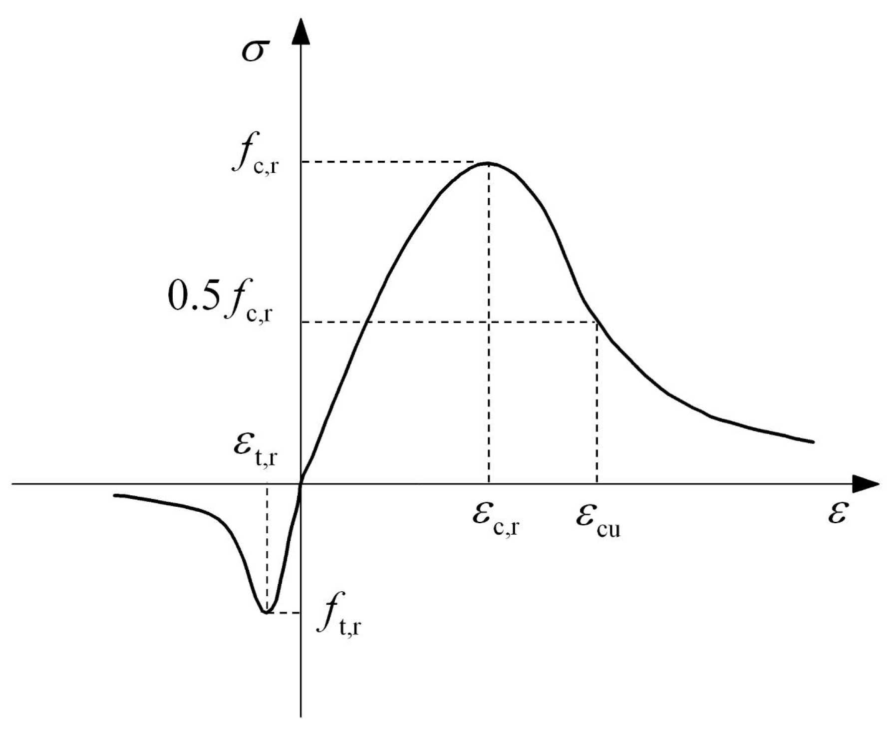
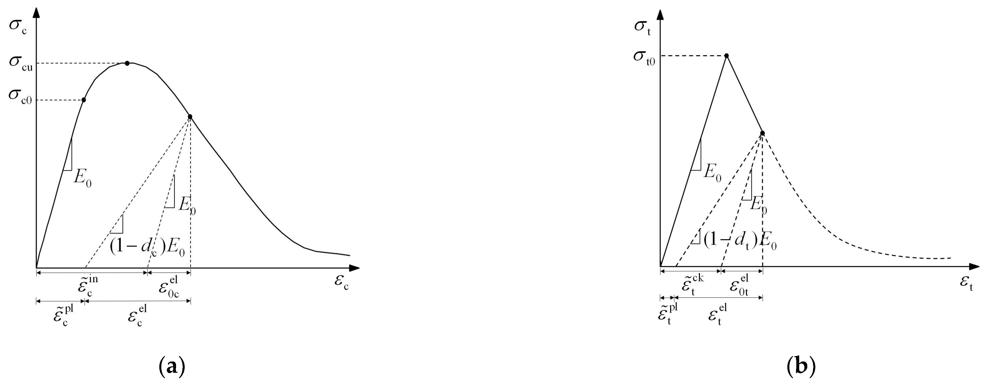
2.4.1. Concrete Constitutive Relations

The compressive and tensile stress–strain curves of concrete, as prescribed in Annex C of GB 50010-2010 [1] and shown in Figure 1, were assigned to the FE models. The concrete uniaxial compressive stress–strain curve can be expressed by Equations (1)–(5), where ${\alpha }_{\mathrm{c}}=0.157f_{\mathrm{c}}^{0.785}-0.905$ is the reference value for the falling branch of the uniaxial compressive stress–strain curve, $d_{\mathrm{c}}^{\prime }$ is the uniaxial compressive damage evolution parameter, $f_{\mathrm{c},\mathrm{r}}$ is the representative uniaxial compressive strength, which can be taken as $f_{\mathrm{c}}$, $f_{\mathrm{ck}}$ or $f_{\mathrm{cm}}$ in different cases, ${\epsilon }_{\mathrm{c},\mathrm{r}}=(700+172\sqrt{f_{\mathrm{c}}})\times {10}^{-6}$ is the concrete peak compressive strength, and $E_{\mathrm{c}}$ is the Young’s modulus of concrete

$$\sigma =(1-d_{\mathrm{c}}^{\prime })E_{\mathrm{c}}\epsilon$$

(1)

$$d_{\mathrm{c}}^{\prime }=\{\begin{array}{ll}1-\frac{{\rho }_{\mathrm{c}}n}{(n-1+x^n)}& x\le 1\\ 1-\frac{{\rho }_{\mathrm{c}}}{{\alpha }_{\mathrm{c}}{(x-1)}^2+x}& x>1\end{array}$$

(2)

$${\rho }_{\mathrm{c}}=\frac{f_{\mathrm{c},\mathrm{r}}}{E_{\mathrm{c}}{\epsilon }_{\mathrm{c},\mathrm{r}}}$$

(3)

$$n=\frac{E_{\mathrm{c}}{\epsilon }_{\mathrm{c},\mathrm{r}}}{E_{\mathrm{c}}{\epsilon }_{\mathrm{c},\mathrm{r}}-f_{\mathrm{c},\mathrm{r}}}$$

(4)

$$x=\frac{\epsilon }{{\epsilon }_{\mathrm{c},\mathrm{r}}}$$

(5)

The concrete uniaxial tensile stress–strain curve [1], can be expressed by Equations (6)–(9), where ${\alpha }_{\mathrm{t}}=0.312f_{\mathrm{t},\mathrm{r}}^2$ is the reference value for the falling branch of the uniaxial tensile stress–strain curve, $d_{\mathrm{t}}^{\prime }$ is the uniaxial tensile damage evolution parameter, $f_{\mathrm{t},\mathrm{r}}$ is the representative uniaxial tensile strength, which can be taken as $f_{\mathrm{t}}$, $f_{\mathrm{tk}}$ or $f_{\mathrm{tm}}$ in different cases, and ${\epsilon }_{\mathrm{t},\mathrm{r}}=f_{\mathrm{t},\mathrm{r}}^{0.54}\times 65\times {10}^{-6}$ is the concrete peak tensile strength.

$$\sigma =(1-d_{\mathrm{t}}^{\prime })E_{\mathrm{c}}\epsilon$$

(6)

$$d_{\mathrm{t}}^{\prime }=\{\begin{array}{ll}1-{\rho }_{\mathrm{t}}(1.2-0.2x^5)& x\le 1\\ 1-\frac{{\rho }_{\mathrm{t}}}{{\alpha }_{\mathrm{t}}{(x-1)}^{1.7}+x}& x>1\end{array}$$

(7)

$$x=\frac{\epsilon }{{\epsilon }_{\mathrm{t},\mathrm{r}}}$$

(8)

$${\rho }_{\mathrm{t}}=\frac{f_{\mathrm{t},\mathrm{r}}}{E_{\mathrm{c}}{\epsilon }_{\mathrm{t},\mathrm{r}}}$$

(9)

The concrete damage plasticity (CDP) model in Abaqus [23] uses different damage factors for tension and compression to describe the stiffness degradation, as shown in Figure 2. The uniaxial compressive stress–strain curve in the CDP model is given by Equations (10)–(12), where $d_{\mathrm{c}}$ is the concrete uniaxial compression damage factor, ${\tilde{\epsilon }}_{\mathrm{c}}^{\mathrm{in}}$ is the concrete compressive inelastic strain, ${\epsilon }_{0\mathrm{c}}^{\mathrm{el}}$ is the concrete compressive elastic strain at initial stiffness, and ${\tilde{\epsilon }}_{\mathrm{c}}^{\mathrm{pl}}$ is the concrete compressive equivalent plastic strain. The uniaxial tensile stress–strain curve equation in the CDP model is given by Equations (13)–(15), where $d_{\mathrm{t}}$ is the concrete uniaxial tension damage factor, ${\tilde{\epsilon }}_{\mathrm{t}}^{\mathrm{ck}}$ is the concrete tensile fracture strain, ${\epsilon }_{0\mathrm{t}}^{\mathrm{el}}$ is the concrete tensile elastic strain at initial stiffness, and ${\tilde{\epsilon }}_{\mathrm{t}}^{\mathrm{pl}}$ is the concrete tensile equivalent plastic strain.

$${\tilde{\epsilon }}_{\mathrm{c}}^{\mathrm{in}}={\sigma }_{\mathrm{c}}-{\epsilon }_{0\mathrm{c}}^{\mathrm{el}}$$

(10)

$${\sigma }_{\mathrm{c}}=\left(1-d_{\mathrm{c}}\right)E_0\left({\epsilon }_{\mathrm{c}}-{\tilde{\epsilon }}_{\mathrm{c}}^{\mathrm{pl}}\right)=E_0{\epsilon }_{0\mathrm{c}}^{\mathrm{el}}$$

(11)

$${\tilde{\epsilon }}_{\mathrm{c}}^{\mathrm{pl}}={\tilde{\epsilon }}_{\mathrm{c}}^{\mathrm{in}}-\frac{d_{\mathrm{c}}}{\left(1-d_{\mathrm{c}}\right)}\frac{{\sigma }_{\mathrm{c}}}{E_0}$$

(12)

$${\tilde{\epsilon }}_{\mathrm{t}}^{\mathrm{ck}}={\sigma }_{\mathrm{t}}-{\epsilon }_{0\mathrm{t}}^{\mathrm{el}}$$

(13)

$${\sigma }_{\mathrm{t}}=\left(1-d_{\mathrm{t}}\right)E_0\left({\epsilon }_{\mathrm{t}}-{\tilde{\epsilon }}_{\mathrm{t}}^{\mathrm{pl}}\right)=E_0{\epsilon }_{0\mathrm{t}}^{\mathrm{el}}$$

(14)

$${\tilde{\epsilon }}_{\mathrm{t}}^{\mathrm{pl}}={\tilde{\epsilon }}_{\mathrm{t}}^{\mathrm{ck}}-\frac{d_{\mathrm{t}}}{\left(1-d_{\mathrm{t}}\right)}\frac{{\sigma }_{\mathrm{t}}}{E_0}$$

(15)

It is clear from Sidiroff energy equivalence principle [25] that the residual elastic energy resulting from a stress of a certain magnitude acting on a damaged material is formally the same as the residual elastic energy resulting from a stress acting on an undamaged material, so the stress or the modulus of elasticity can be changed to the effective stress or the equivalent modulus of elasticity at the time of damage when calculating the damage factor, using Equations (16) and (17). The results of damage factor calculations using the equivalent modulus of elasticity at effective stress or damage are the same. $W_0^e$ is the residual elastic energy in the undamaged case, $W_{\mathrm{d}}^e$ is the residual elastic energy in the damaged case, and $\overline{\sigma }={(1-d)}^2\sigma$ is the effective stress considering damage. Using Equations (16) and (17) can lead to $E_{\mathrm{d}}=E_0(1-d)$ and Equations (18) and (19). The concrete uniaxial compression damage factor $d_{\mathrm{c}}$ and the concrete uniaxial tension damage factor $d_{\mathrm{t}}$ can be derived by coupling Equations (1) and (6) with Equation (19).

$$W_0^e=\frac{{\sigma }^2}{2E_0}$$

(16)

$$W_{\mathrm{d}}^e=\frac{{\overline{\sigma }}^2}{2E_{\mathrm{d}}}$$

(17)

$$\sigma =E_0{\left(1-d\right)}^2\epsilon$$

(18)

$$d=1-\sqrt{\frac{\sigma }{E_0\epsilon }}$$

(19)

In the modelling of the ABAQUS CDP model, parameters such as Poisson’s ratio, angle of dilatancy and flow potential offset value need to be defined. Reference [26] has fully discussed these parameters, so it can be considered that these parameters are credible. And these parameters can be inputted according to

Table 1. Parameters for CDP Model.

$\mathit{\upsilon }$	$\mathit{\psi }$	∈	σb0/σc0	${\mathit{{\rm K}}}_{\mathbf{c}}$	$\mathit{\mu }$
0.2	40	0.1	1.16	0.667	0.0005

Note: $\mathit{\upsilon }$ is the Poisson’s ratio; $\mathit{\psi }$ is the angle of dilatancy; ∈ is flow potential offset value, σ_b0/σ_c0 is the biaxial-to-uniaxial ultimate compressive stress ratio, ${\mathit{{\rm K}}}_{\mathbf{c}}$ is the shape factor, and $\mathit{\mu }$ is the viscosity factor.

.

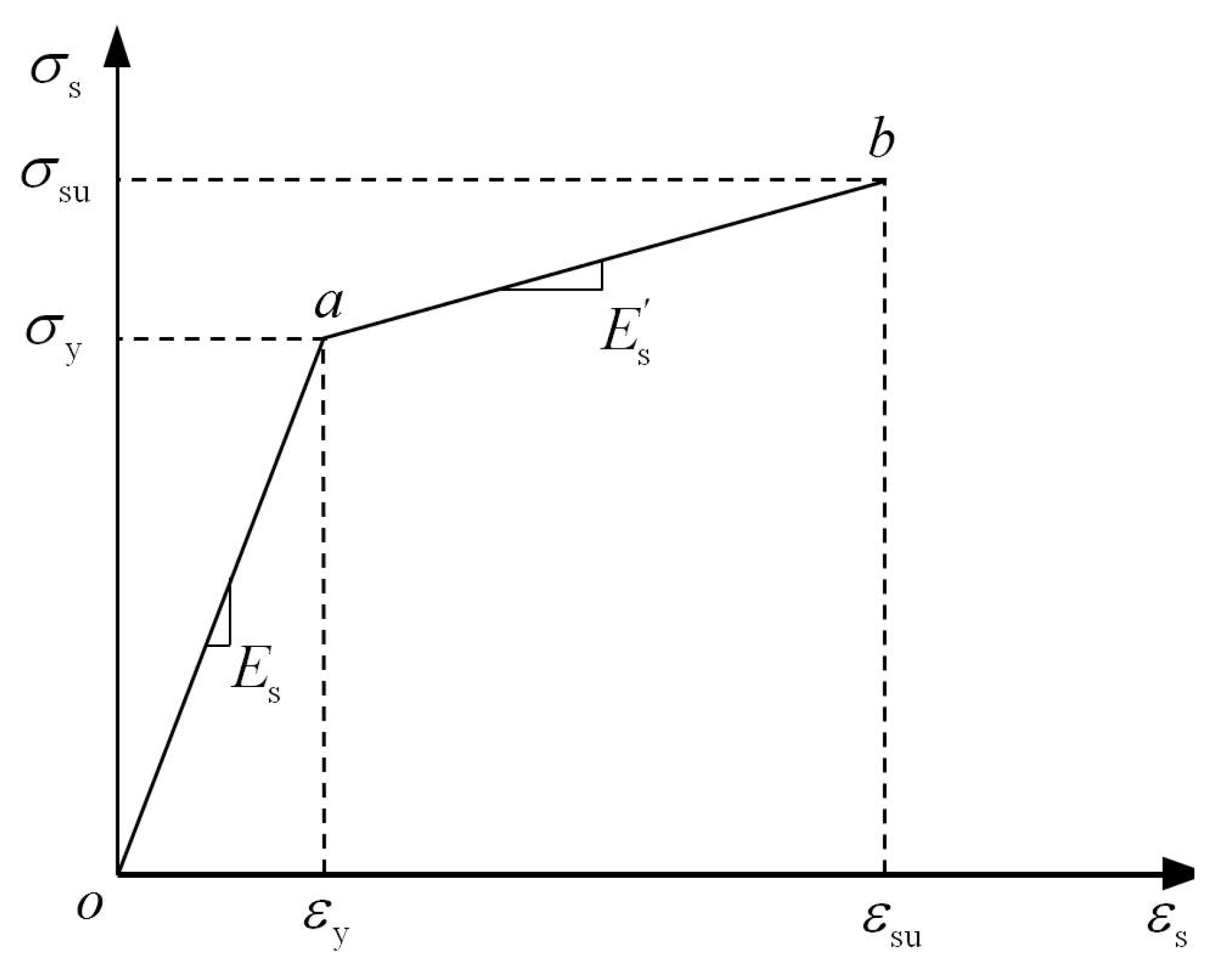
2.4.2. Reinforcement Constitutive Relations

In Abaqus, there are three commonly used types of steel constitutive models, including the elasto-plastic model, the bi-linear hardening model and the tri-linear elasto-plastic hardening model. The bi-linear hardening model can better simulate the real situation than the elasto-plastic model and is less computationally intensive and easier to converge than the tri-linear elasto-plastic hardening model. Therefore, the bi-linear hardening model [1], was utilised in this study, as shown in Figure 3. In Figure 3, the “oa” portion represents the elastic stage of the stress–strain curve, while the “ab” portion represents the hardening stage of the stress–strain curve, where the initial Young’s modulus of steel $E_{\mathrm{s}}$ is equal to 2 × 10⁵ MPa and the Poisson’s ratio of steel is equal to 0.3. The steel stress–strain curve can be expressed by Equations (20) and (21), where is ${\sigma }_{\mathrm{y}}$ the steel yield stress and can be taken as $f_{\mathrm{y}}$ or $f_{\mathrm{yk}}$, ${\sigma }_{\mathrm{su}}$ is the steel ultimate stress and is taken as $f_{\mathrm{stk}}$, $E_{\mathrm{s}}^{\prime }$ is the strain hardening Young’s modulus, ${\epsilon }_{\mathrm{y}}$ is the yield strain corresponding to the yield stress ${\sigma }_{\mathrm{y}}$, and ${\epsilon }_{\mathrm{su}}$ is the ultimate strain.

$${\sigma }_{\mathrm{s}}=E_{\mathrm{s}}{\epsilon }_{\mathrm{s}} \mathrm{for} {\epsilon }_{\mathrm{s}}\le {\epsilon }_{\mathrm{y}}$$

(20)

$${\sigma }_{\mathrm{s}}={\sigma }_{\mathrm{y}}+E_{\mathrm{s}}^{\prime }\left({\epsilon }_{\mathrm{s}}-{\epsilon }_{\mathrm{y}}\right) \mathrm{for} {\epsilon }_{\mathrm{y}}<{\epsilon }_{\mathrm{s}}\le {\epsilon }_{\mathrm{s}}$$

(21)

3. Validation of FE Simulation Method

There have been extensive experimental studies on slab-column joints. In this paper, FE models were developed based on the tested specimens reported in previous studies, and then analysed to derive numerical results. The obtained numerical results were compared against the corresponding test results, in order to evaluate the suitability and accuracy of the developed FE models.

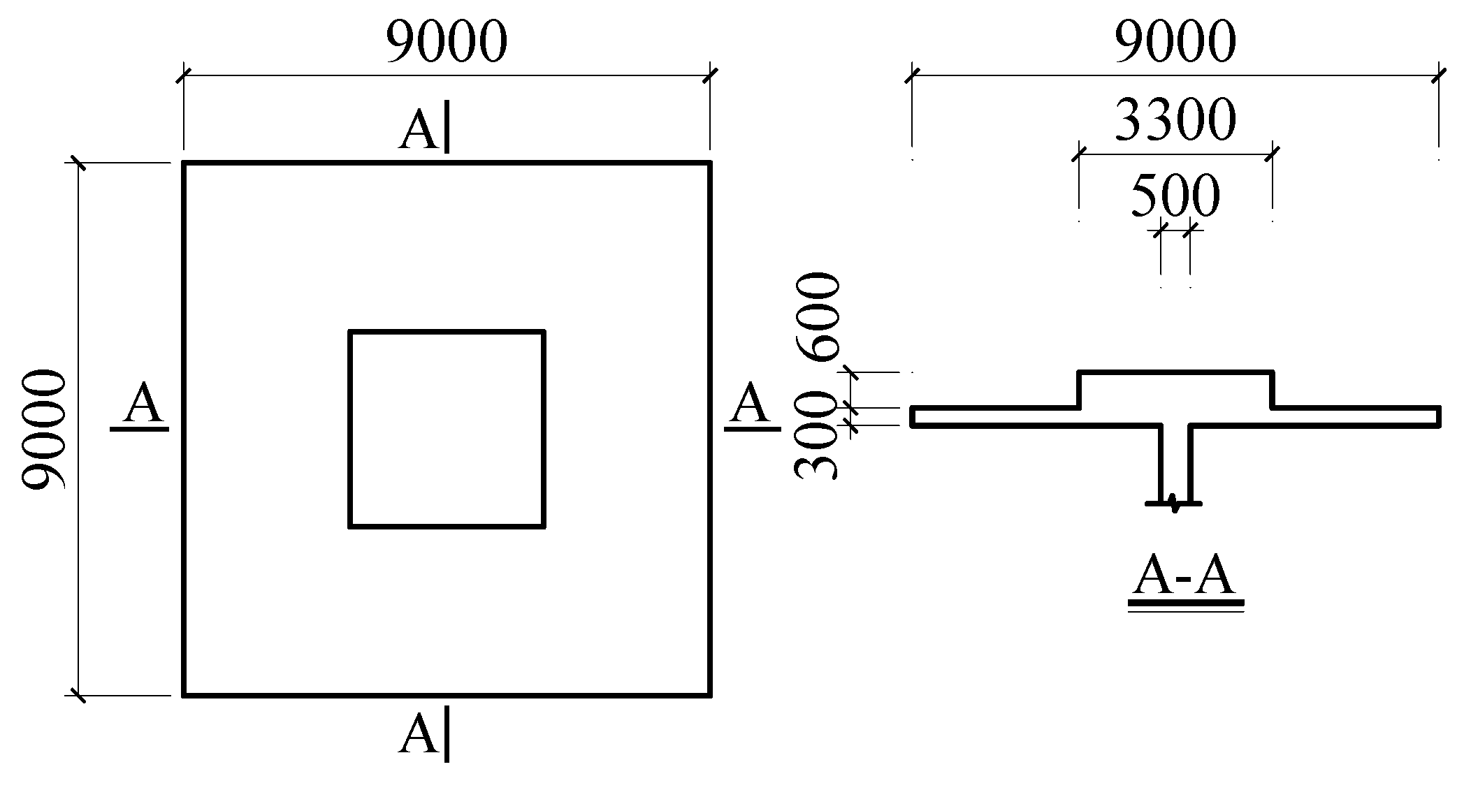
3.1. Overview of Test and Development of FE Models

Specimen SB1 reported in reference [11] was selected to verify the aforementioned FE simulation method. The specimen is shown in Figure 4 and the reinforcements have been detailed in [11]. According to reference [26], displacement-controlled loading was applied on column end. The average values of experimentally obtained material properties are presented in

Table 2. Material Properties of Specimen SB1.

Concrete			Reinforcement
$f_{\mathrm{ck}}$ (MPa)	$f_{\mathrm{tk}}$ (MPa)	$E_{\mathrm{c}}$ (MPa)	$f_{\mathrm{yk}}$ (MPa)	${\epsilon }_{\mathrm{y}}$	$f_{\mathrm{stk}}$ (MPa)	${\epsilon }_{\mathrm{su}}$
44	2.2	36880	455	0.0023	650	0.25

. The FE modelling was conducted by means of the aforementioned FE simulation method and using the experimentally obtained material properties in Table 2. The boundary conditions and loading conditions are depicted in Figure 5.

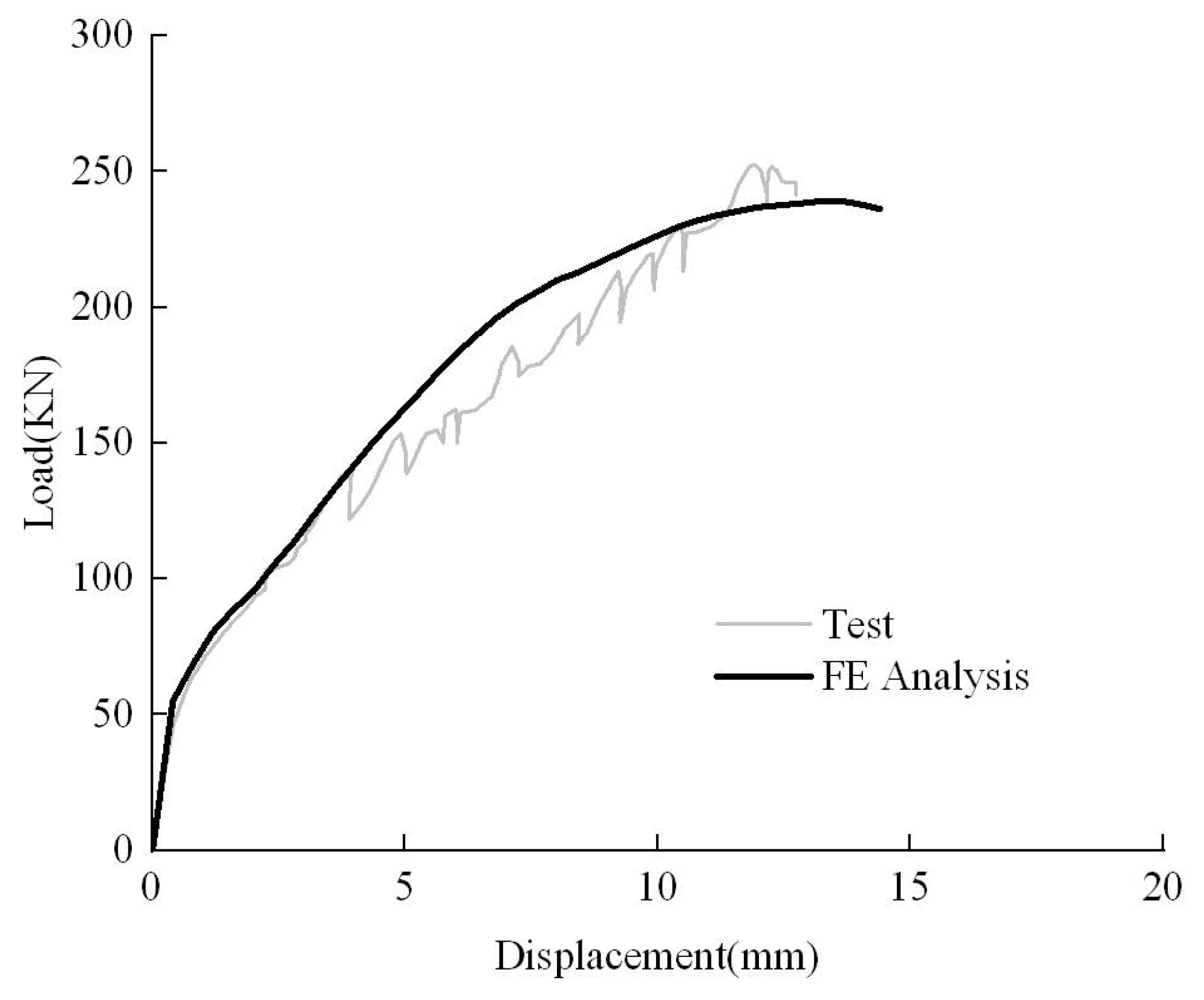
3.2. Comparison of Test and FE Results

The test and FE load–displacement curves of specimen SB1 are shown in Figure 6. The FE model displayed the same brittle punching shear failure as observed in the test. It was also observed that the FE model exhibited higher stiffness than the test specimen, which may be contributed to (i) the existence of initial microcracks in the concrete prior to the test and (ii) no consideration of the slip between the reinforcement and the concrete in modelling. The ultimate loads and ultimate displacements obtained from the test and FE simulation are presented in

Table 3. Test and FE Results.

Specimen	Test		FE Simulation
	Ultimate Load (kN)	Ultimate Displacement (mm)	Ultimate Load (MPa)	Ultimate Displacement (mm)
SB1	44	2.2	455	0.0023

. The ultimate load discrepancy is 5.54% and the ultimate displacement discrepancy is 14.29%. These results are generally consistent with the FE simulation results reported in Reference [11]. The ultimate displacement discrepancy is 1.7 mm, which is an acceptable value, due to the error of the measuring instrument.

The numerically obtained cracking patterns of the tensile side of the concrete slab at failure are shown in Figure 7. The cracks occurred tangentially in the vicinity of the column, developed within the slab adjacent to the column, and then tended to extend radially with increasing displacement. At the ultimate load, a punching cone was formed due to the development of cracks. This phenomenon is consistent with the development of concrete cracks observed in the test and the punching shear failure was also observed in the test. Therefore, the adopted FE simulation method can be considered to be accurate and applicable.

4. Mechanical Performance Analysis of Slab-Column Joints

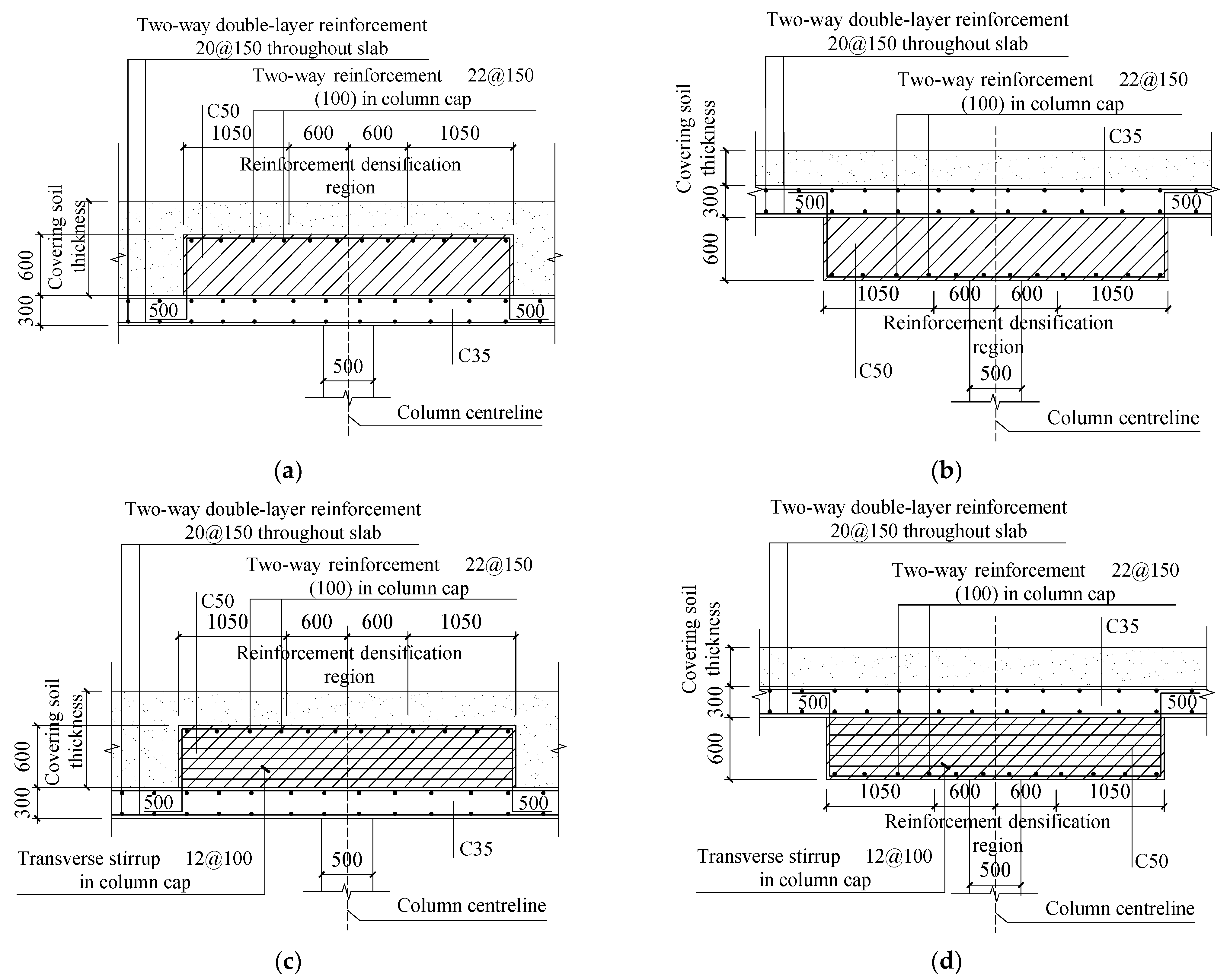
4.1. Analysis of FE Models

The aforementioned FE simulation method was used to simulate the slab-column joint employed in an engineering practice of cast-in-situ reinforced concrete flat slab structure with reverse column cap, with a column grip of 9 m × 9 m. The same dimensions were adopted to develop an FE model on the slab-column joint with traditional column cap. Then, two additional FE models were developed by arranging transverse stirrups. Specifically, specimen ZM01 is the reverse column cap without transverse stirrups, as shown in Figure 8; specimen ZM02 is the conventional column cap without transverse stirrups; specimen ZM03 is the reverse column cap with transverse stirrups; specimen ZM04 is the conventional column cap with transverse stirrups. The reinforcement arrangement in specimens ZM01–ZM04 are detailed in Figure 9. The FE model for specimen ZM01 is shown in Figure 10. According to Table 4.1.3-1, Table 4.1.3-2 and Table 4.2.2-1 of GB50010-2010 [1], the material properties assigned to the concrete and reinforcements of FE models are presented in

Table 4. Material properties of concrete.

Concrete Grade	${\mathit{f}}_{\mathbf{ck}} \left(\mathbf{MPa}\right)$	${\mathit{f}}_{\mathbf{tk}} \left(\mathbf{MPa}\right)$	${\mathit{E}}_{\mathbf{c}} \left(\mathbf{MPa}\right)$
C35	23.4	2.20	31,500
C50	32.4	2.64	34,500

and

Table 5. Material properties of Reinforcement.

Reinforcement Grade	${\mathit{f}}_{\mathbf{yk}} \left(\mathbf{MPa}\right)$	${\mathit{\epsilon }}_{\mathbf{y}}$	${\mathit{f}}_{\mathbf{stk}} \left(\mathbf{MPa}\right)$	${\mathit{\epsilon }}_{\mathbf{su}}$
HRB400	400	0.002	540	0.02

.

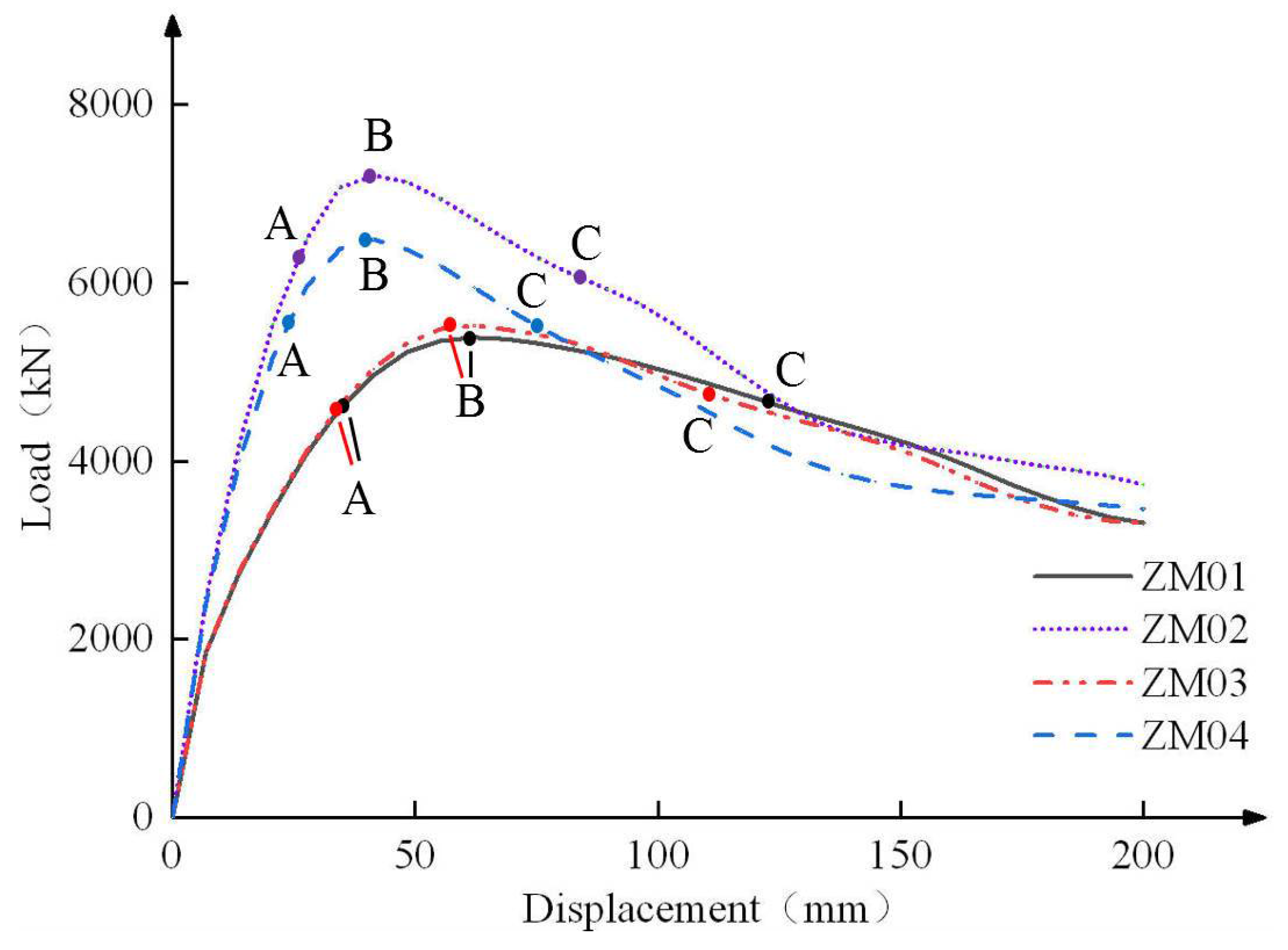
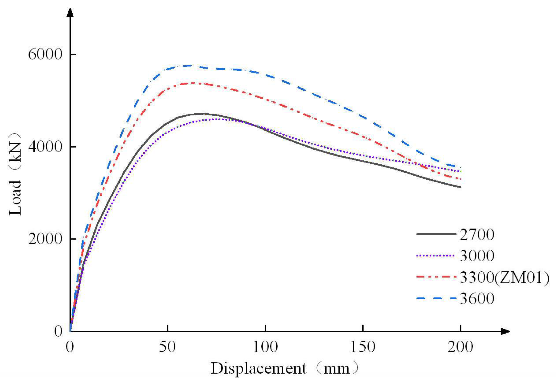
4.2. Comparison of Load–Displacement Curves

Vertical loading was applied to the FE models of specimens ZM01–ZM04 at displacement control and the derived FE load–displacement curves are shown in Figure 11. It can be seen from Figure 11 that the slope of each curve gradually decreases until the attainment of ultimate load, indicating that all the specimens experienced some damage with the increase of displacements, leading to reduced stiffness. The ultimate loads of specimens ZM02 and ZM04 with conventional column cap were significantly higher than those of specimens ZM01 and ZM03 with reverse column cap, and their ultimate displacements corresponding to the ultimate loads were smaller than those of specimens ZM01 and ZM03. Compared with specimen ZM01, the load-carrying capacity of specimen ZM03 with transverse stirrups in the column cap is not significantly enhanced. The load-carrying capacity of specimen ZM04 with transverse stirrups in the column cap is lower than that of specimen ZM02, while their ultimate displacements corresponding to the ultimate loads are almost the same. The above-mentioned shows that the slab-column joints with conventional caps are superior to their counterparts with reverse caps in terms of the load-carrying capacities.

According to the equivalent energy method [27], namely replacing the original curve with an elasto-plastic bi-linear curve with the same envelope area, the displacement at the inflection point of the bi-linear curve is taken as the yield displacement and the corresponding point on the original curve is defined yield point. The yield point of each curve can then be determined based on Figure 11. According to Clause 4.4.4 of JG J101-2015 [28], it is suggested that tests for determining load-carrying capacity and damage characteristics at the limit state should be carried out until the falling branch of the test curve attains 85% of the ultimate load. As a result, the point at which the load value is 85% of the ultimate load is considered to be the failure point. The ductility factor, reflecting the capacity of the structural component if the capacity is not significantly decreased, can be expressed as the ratio of the failure displacement to the yield displacement.

Table 6. FE results for specimens ZM01–ZM04.

Specimen	Yield Point		Ultimate Point		Failure Point		Ductility Factor	Failure Mode
	Yiled Displacement (mm)	Yield Load (kN)	Ultimate Displacement (mm)	Ultimate Load (kN)	Failure Displacement (mm)	Failure Load (kN)
ZM01	34.12	4565.48	63.34	5385.29	127.33	4577.19	3.73	Flexure
ZM02	26.13	6308.72	39.82	7204.04	81.33	6123.43	3.11	Flexure
ZM03	35.10	4653.22	61.02	5518.26	113.85	4690.52	3.24	Flexure
ZM04	24.51	5648.88	40.65	6486.50	74.98	5513.53	3.06	Flexure

presents the FE results for specimens ZM01–ZM04. It is evident in Table 6 that specimens ZM01 and ZM03 with reverse cap have higher deformation capacity than specimens ZM02 and ZM04 with conventional cap, but they possess lower ultimate capacity. For the slab-column joints with reverse cap, the ultimate load of specimen ZM03 with transverse stirrups in cap is increased by 2.4% compared to that of specimen ZM01 without transverse stirrups in cap, but the ductility is decreased by 13.4%. For the slab-column joints with conventional cap, the ultimate load of specimen ZM04 with transverse stirrups in cap is decreased by 10.0% compared to that of specimen ZM02 without transverse stirrups in cap, and the ductility is decreased by 1.6%. In addition, the failure mode of specimens ZM01–ZM04 is different from the punching failure of common slab-column joints [26,29], which is flexure failure. This may be caused by the large depth of column cap. Table 6 also shows that the arrangement of transverse stirrups in the column cap has limited effect on the load-carrying capacity of the slab-column joints with reverse cap; instead, this weakens the joint ductility. The arrangement of transverse stirrups in the column cap has negative impact on the load-carrying capacity and ductility of the slab-column joints with conventional cap.

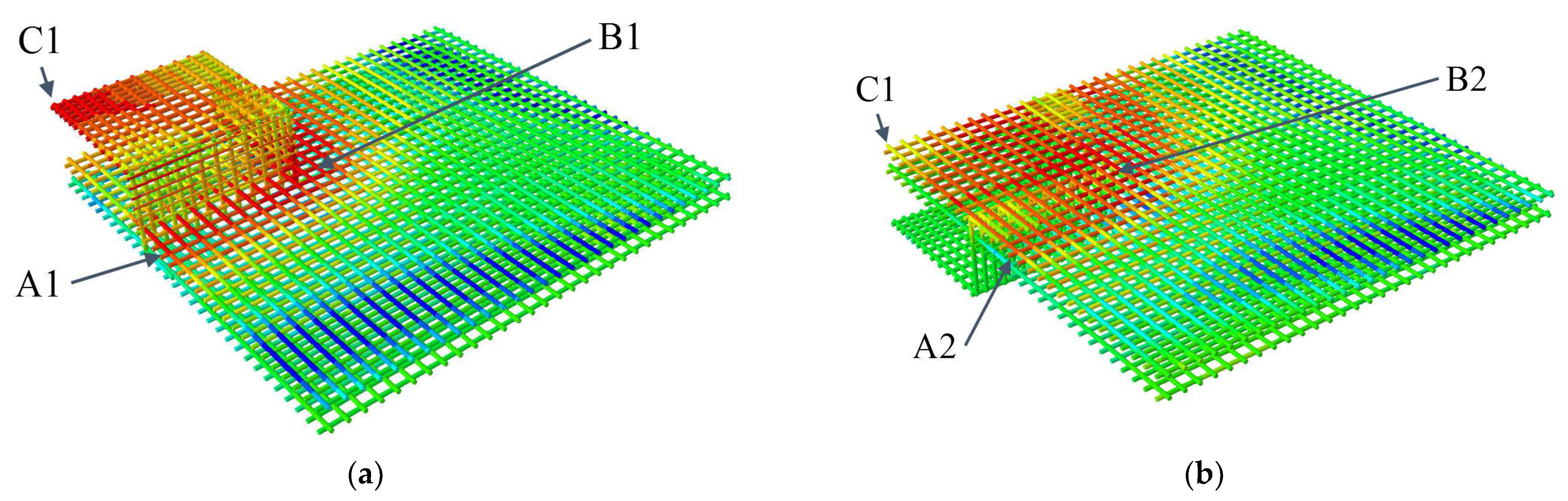
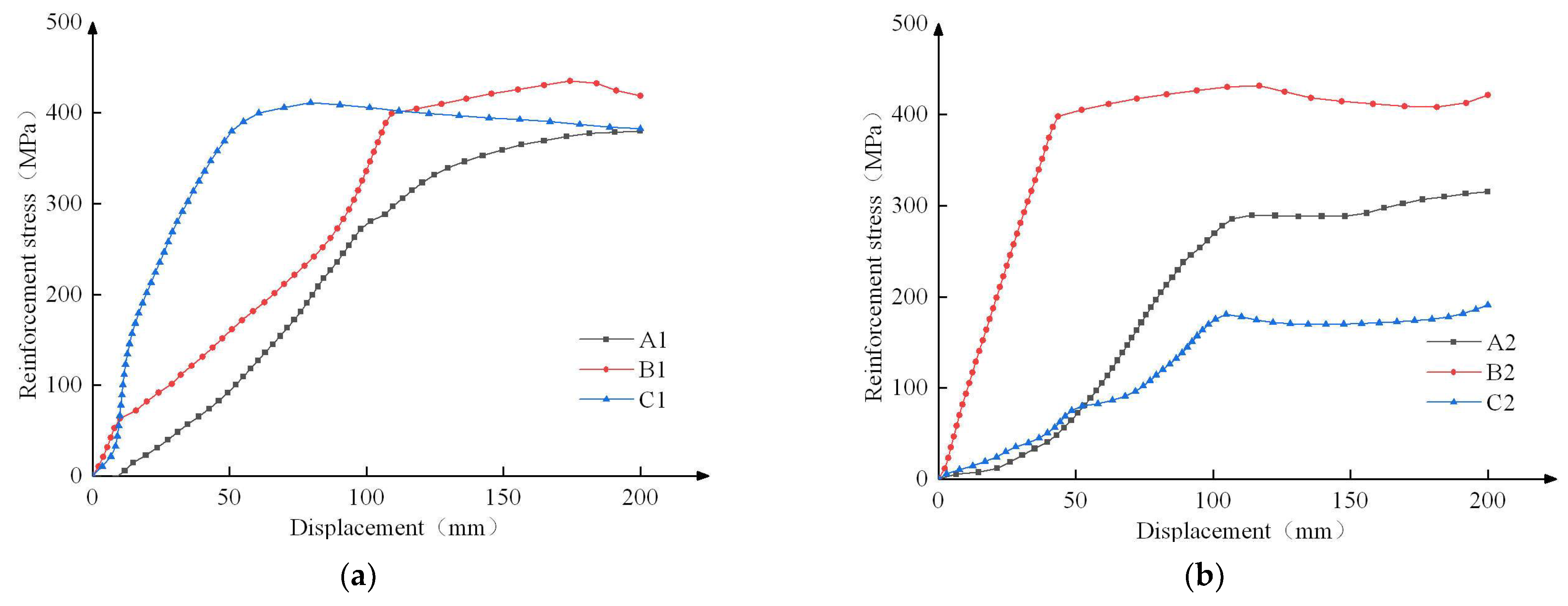
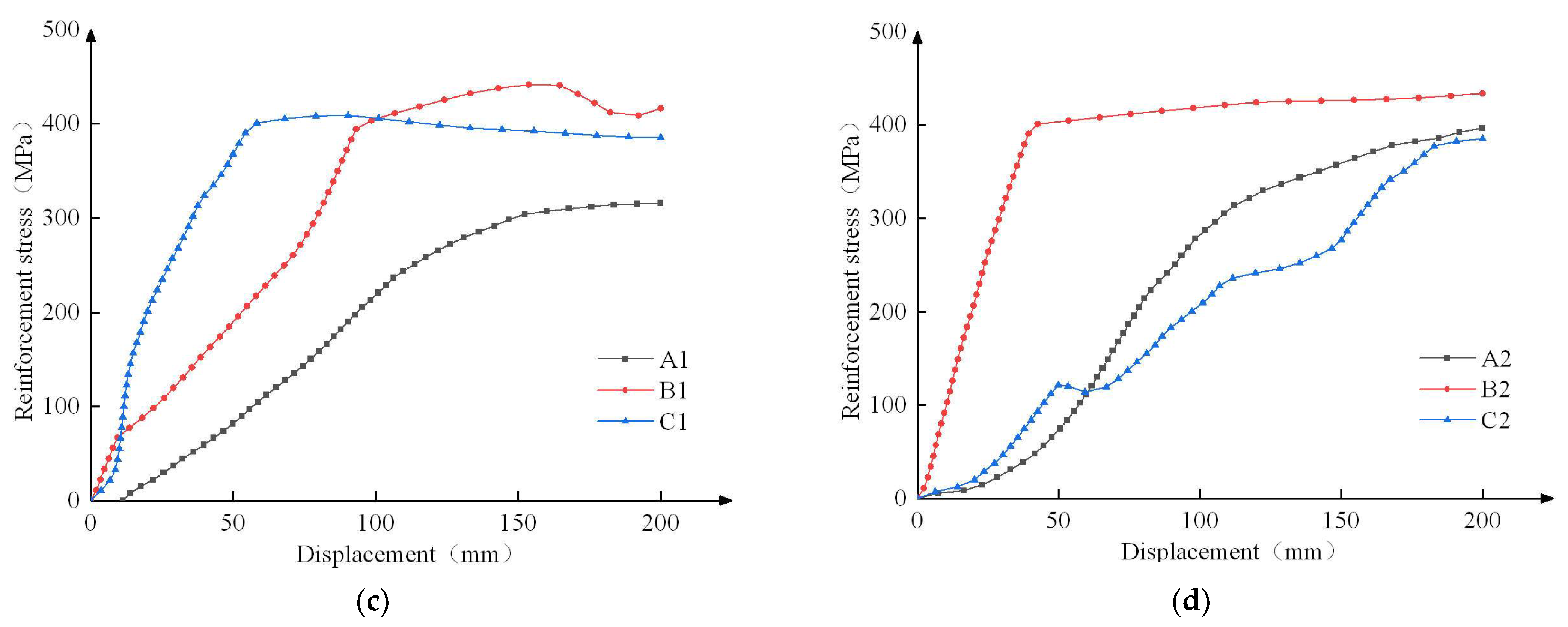
4.3. Comparison of Stress Change in Reinforcement

According to the FE results, with the increase of displacement, the relatively higher stresses in the specimen reinforcements are shown in Figure 12. For specimens ZM01 and ZM03, the slab surface reinforcements at the column cap edge centre, the slab surface reinforcements corresponding to the column cap corner, and the column cap reinforcements at the centre of the column cap are respectively denoted as A1, B1 and C1. For specimens ZM02 and ZM04, the slab surface reinforcements at the column cap edge centre, the slab surface reinforcements corresponding to the column cap corner, and the slab surface reinforcements at the centre of the column are respectively denoted as A2, B2 and C2.

The stress–load curves for the corresponding reinforcements in each specimen are shown in Figure 13. As can be seen from Figure 13, the central column cap reinforcements (C1) govern the structural behaviour of specimens ZM01 and ZM03, while the slab surface reinforcements corresponding to the column cap corner (B2) govern the structural behaviour of specimens ZM02 and ZM04. When the reinforcements C1 and B2 reach the yield stress, the specimens also reach their ultimate loads.

Table 7. Displacements corresponding to reinforcement stresses reaching yield stress.

Specimen	Displacements (mm)
	A1/A2	B1/B2	C1/C2
ZM01	-	109.88	61.03
ZM02	-	44.03	-
ZM03	-	93.91	57.83
ZM04	-	40.65	-

reports the displacements corresponding to the stresses in the reinforcements reaching the yield stress. After the stresses of the reinforcements C1 in specimens ZM01 and ZM03 reach the yield stress, the stresses of the reinforcements B1 continue to increase until they reach the yield stress. When the reinforcements B1 in specimen ZM03 reach the yield stress, they have smaller displacements compared against their counterparts in specimen ZM01, and the stresses of the reinforcements A1 in specimen ZM03 are lower than their counterparts in specimen ZM01. This indicates that the column cap stirrups can effectively restrain the column cap concrete and limit the horizontal outward movement of the concrete and column cap reinforcement, making the column cap relatively less susceptible to deformation. For specimen ZM01, the load is jointly carried by the reinforcements A1 and B1 when the column cap deforms. Similarly, when the reinforcements B2 in specimen ZM04 reach the yield stress, they have smaller displacements compared against their counterparts in specimen ZM02. However, since the column cap has larger stiffness, the slab cannot bend toward the column cap. At the same time, the inward extrusion of the concrete in the column cap increases the stresses in the reinforcements C2, as reflected by the fact that the C2 stresses in specimen ZM04 are greater than those in specimen ZM02.

The column cap stirrups increase the stiffness of column cap, resulting in that the internal force of the reverse column cap joint converges to the diagonal, which is unfavourable for the slab to carry the load. However, the critical position of the reverse column cap joint is at the column cap, and the column cap with larger stiffness can improve the load-carrying capacity of the joint. Moreover, the column cap with larger stiffness can increase the internal force of the slab at the column centre and reduce the corresponding load-carrying capacity. Therefore, in the design of the slab-column joint with reverse cap, the cap stiffness can be enhanced by increasing the concrete strength and arranging cap stirrups. However, the slab-column joint with conventional cap may not adopt the cap with excessively large stiffness.

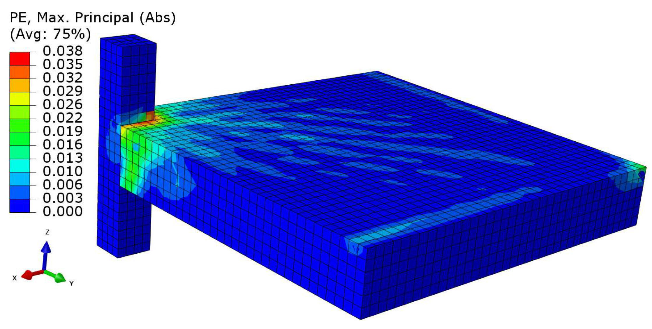
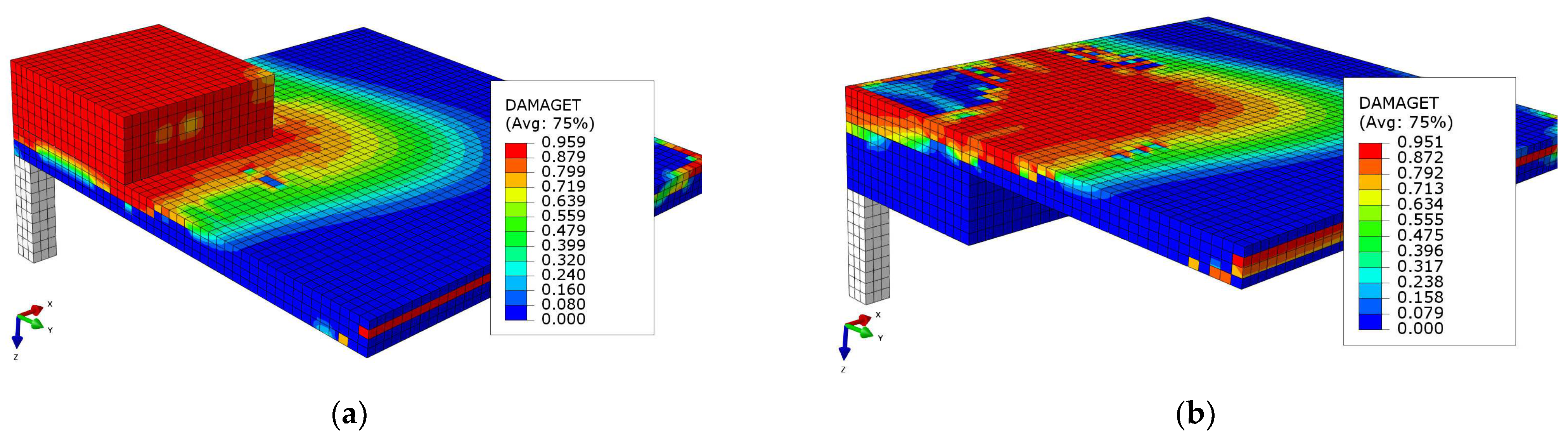
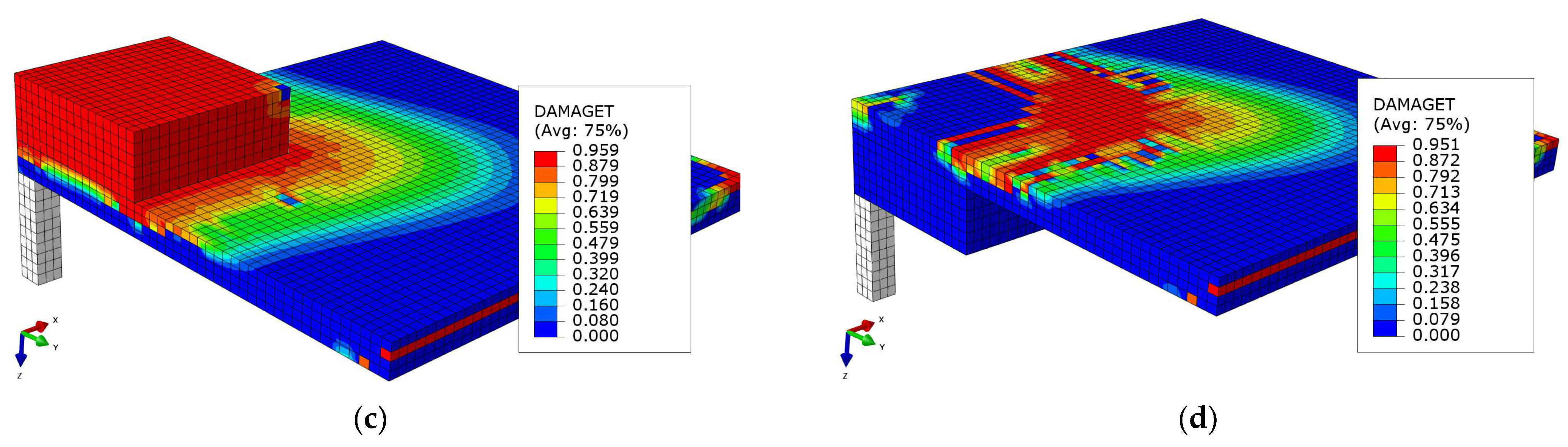
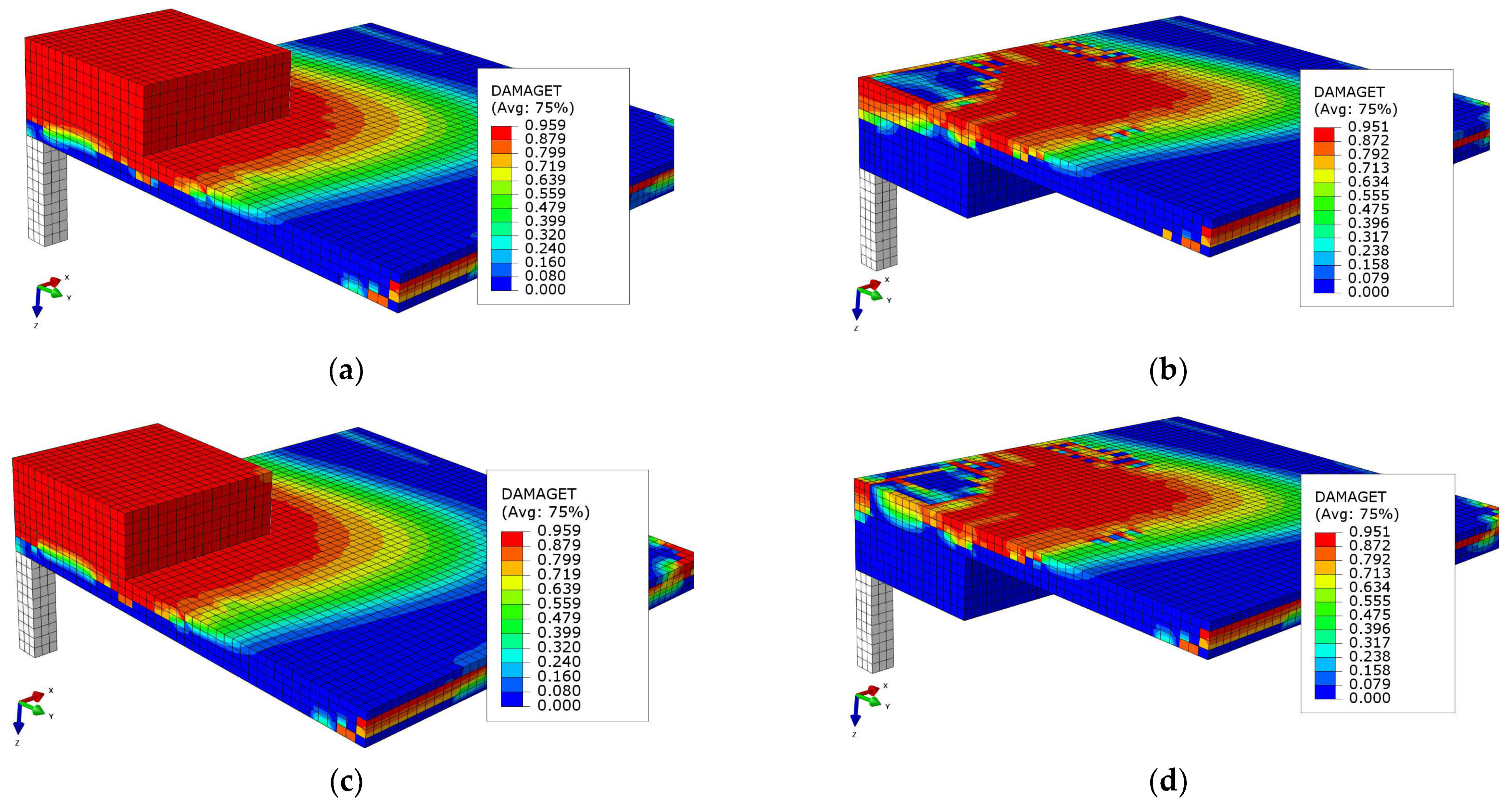
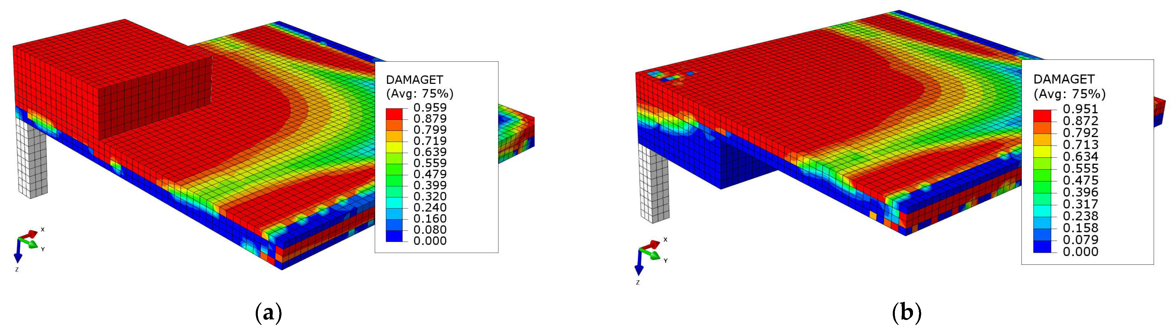
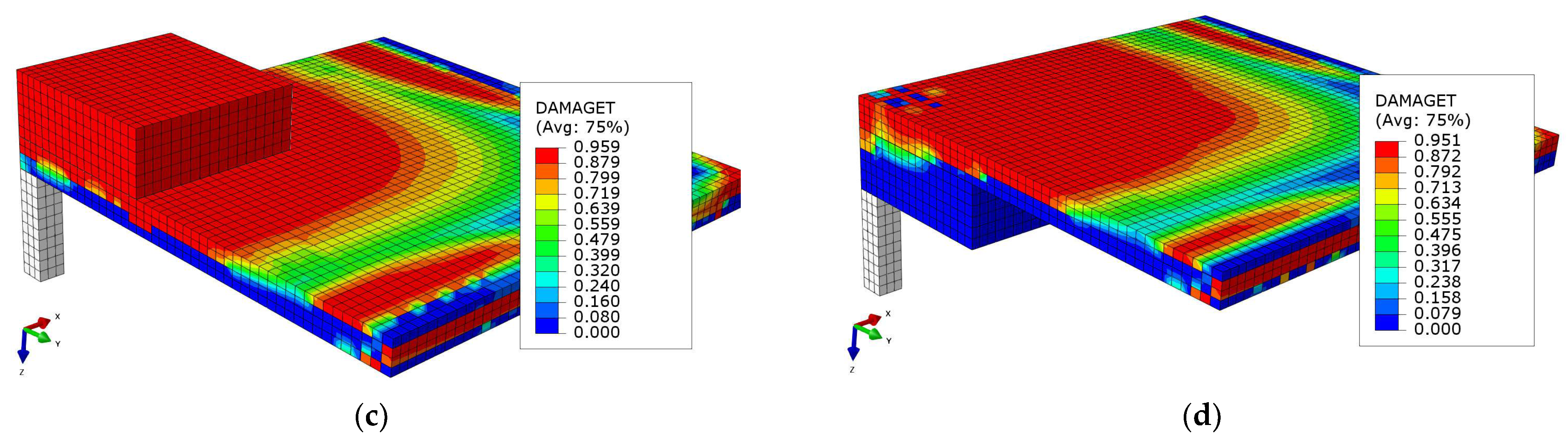
4.4. Development of Concrete Tensile Damage

Figure 14, Figure 15 and Figure 16 show the tensile damage diagrams of the tensile sides of specimens ZM01–ZM04 at yield load, ultimate load and failure load. It can be seen that the position of tensile damage of the concrete in the reverse column caps is not the same as that of the conventional column caps, indicating the difference in load-carrying scheme. For the reverse column caps, the tensile damage firstly occurs at the column cap and then radially develops, with very little damage to the slab concrete corresponding to the column caps. In comparison, the tensile damage firstly occurs in the slabs at the column cap edges, and then develops simultaneously towards the column centre and edges, with a tendency to develop towards the column cap. This is different from the references [26,29], in which concrete tensile damage first occurs at the slab-column joints. Therefore, in the design of slab-column structures with column caps, attention should be paid to strengthening the stiffness of the reverse column cap, and to strengthening the slab at the edge of the conventional column cap.

4.5. Parametric Analysis

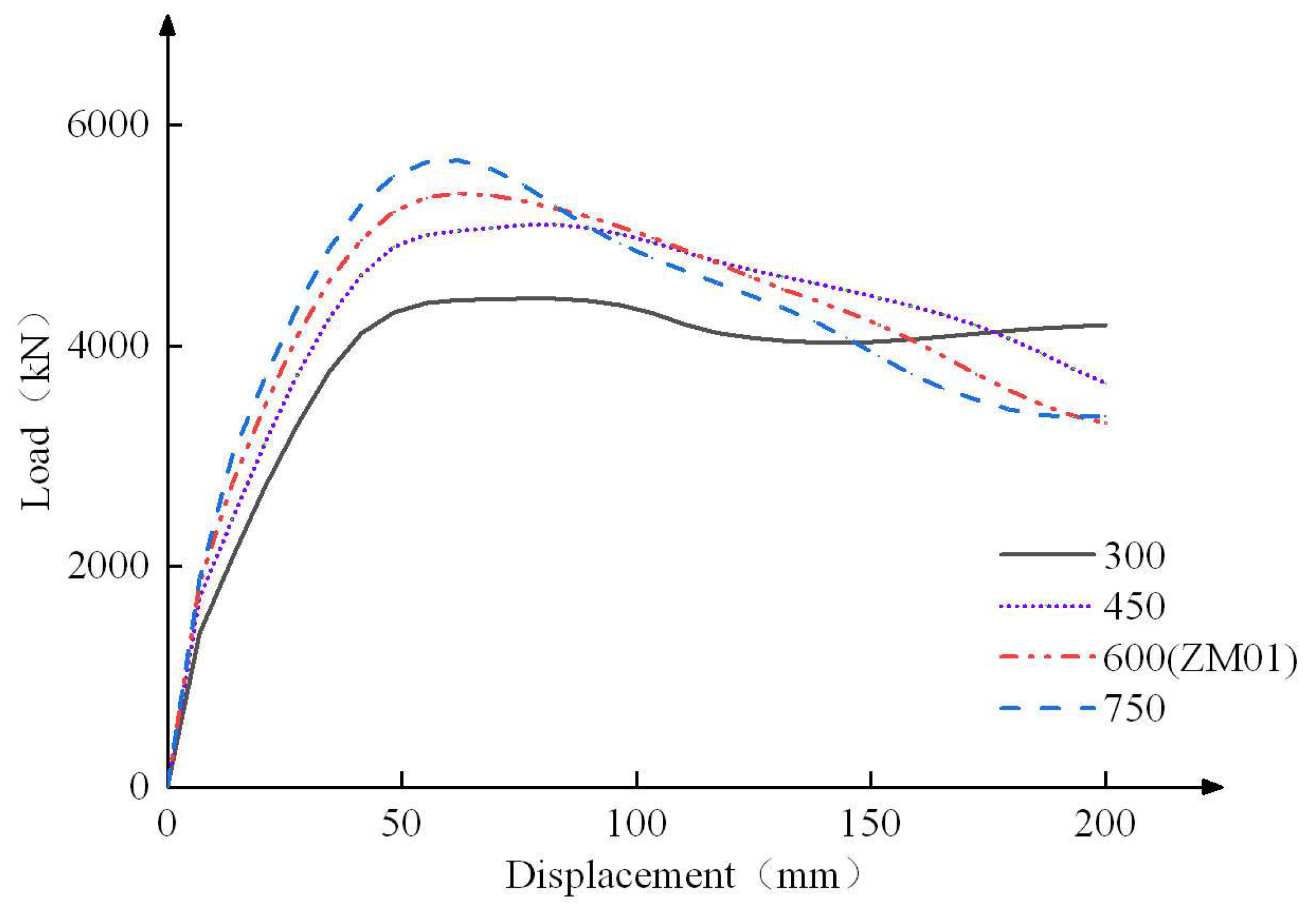
4.5.1. Size of Column Cap

Based on specimen ZM01, the column cap size is changed to 2700 mm, 3000 mm and 3600 mm, respectively, with the load-displacement curves compared in Figure 17. It was found that the ultimate loads of slab-column joints became higher with the increase of cap size except for the one with the cap size of 2700 mm. This indicates that increasing the size of column caps can effectively improve the bearing capacity of slab-column joints. On the other hand, the ultimate displacements are insensitive to the changes in the parameter, meaning the size of column cap is not the significant factor in influencing the ultimate displacements of slab-column joints.

4.5.2. Depth of Column Cap

Based on specimen ZM01, three column cap depths are investigated, which are 300 mm, 450 mm and 750 mm, respectively. Their load-displacement curves were obtained by using the above simulation method and compared with the load-displacement curve of specimen ZM01 (Figure 18). It can be seen that the increment of the ultimate load becomes smaller as the depth of column cap increases, meaning that the improvement of the bearing capacity of slab-column joints is not controlled by the depth of column cap in a high depth of column cap. After the ultimate load, the curves drop at different slopes. As the depth of the column cap increases, the curves descend fast, which illustrates that the ductility of the slab-column joint with the deeper column cap becomes worse. When the depth of the column cap is the same as the flat slab thickness, there is a second ultimate load after the first ultimate load, meaning that the column cap may not be the only control position in the slab-column joint with the reverse column cap.

5. Design

5.1. Punching Shear Design Provisions

Three design codes are considered in this section to determine the punching shear resistance of the slab-column joints. The predicted punching shear resistances were then compared against the FE results, allowing the accuracy of the three design codes to be assessed. The formulations given in GB50010 [1], EC2 [7] and ACI318 [8] are summarized in

Table 8. Design codes for punching shear resistance.

Design Codes	Punching Shear Strength	Note
GB50010 [1]	$V_{\mathrm{GB}}=0.7{\beta }_{\mathrm{h}}{f}_{\mathrm{t}}\eta u_{\mathrm{m}}{h}_0$ $\eta =\min \{\begin{array}{l}{\eta }_1=0.4+\frac{1.2}{{\beta }_{\mathrm{s}}}\\ {\eta }_2=0.5+\frac{{\alpha }_{\mathrm{s}}{h}_0}{4u_{\mathrm{m}}}\end{array}$	The section height influence coefficient βh = 0.9–1.0; η1 is the influence coefficient of the shape of loaded area; η2 is the influence coefficient (um/h0).	um is the critical perimeter, taken at distance 2d for EC2, and taken as distance d/2 for GB50010 and ACI318; h0 is the effective depth; αs is the column position influence coefficient, which is taken as 40, 30 and 20 for the inner, edge and corner columns, respectively; βs is the ratio of long side to short side.
EC2 [7]	$\begin{array}{c}{V}_{\mathrm{EC}}=\frac{1}{{\alpha }_{\mathrm{sc}}}\left[0.18k{\left(100\rho f_c^{\prime }\right)}^{1/3}-0.1\sigma \right]u_{\mathrm{m}}{h}_0\\ \ge \frac{1}{{\alpha }_{\mathrm{sc}}}\left(0.028k^{3/2}\sqrt{f_c^{\prime }}-0.1\sigma \right)u_{\mathrm{m}}{h}_0\end{array}$	${\alpha }_{\mathrm{sc}} \mathrm{is} \mathrm{the} \mathrm{column} \mathrm{position} \mathrm{influence} \mathrm{coefficient}, \mathrm{which} \mathrm{is} \mathrm{taken} \mathrm{as} 1.15, 1.4 \mathrm{and} 1.5 \mathrm{for} \mathrm{the} \mathrm{inner}, \mathrm{edge} \mathrm{and} \mathrm{corner} \mathrm{columns}; k=1+{\left(200/h_0\right)}^{0.5}\le 2 \mathrm{is} \mathrm{the} \mathrm{size} \mathrm{effect} \mathrm{coefficient}; \rho \mathrm{is} \mathrm{flexure} \mathrm{reinforcement} \mathrm{ratio} \mathrm{taken} \le 2\%; \sigma \mathrm{is} \mathrm{the} \mathrm{normal} \mathrm{concrete} \mathrm{stress} \mathrm{due} \mathrm{to} \mathrm{membrane} \mathrm{forces}.$
ACI318 [8]	$V_{ACI}=smallest of\{\begin{array}{l}0.17\left(1+\frac{2}{\beta \mathrm{s}}\right)\lambda \mathrm{s}\sqrt{f_c^{\prime }}{u}_{\mathrm{m}}{h}_0\\ 0.33\lambda \mathrm{s}\sqrt{f_c^{\prime }}{u}_{\mathrm{m}}{h}_0\\ 0.083\left(2+\frac{{\alpha }_{\mathrm{s}}{h}_0}{u_{\mathrm{m}}}\right)\lambda \mathrm{s}\sqrt{f_c^{\prime }}{u}_{\mathrm{m}}{h}_0\end{array}$	$\lambda \mathrm{s}$$\mathrm{is} \mathrm{the} \mathrm{size} \mathrm{effect} \mathrm{factor}, \mathrm{which} \mathrm{is} \mathrm{calculated} \mathrm{as} \sqrt{\frac{2}{1+0.0004d}}\le 1.$

. In general, the shape of the punching shear critical section, the size of the critical section, the effective depth, the reinforcement ratio, and other controlling factors have been considered in these three design codes, in which the effective height h₀ of the slab [19] is the controlled parameter relating to the punching shear capacity.

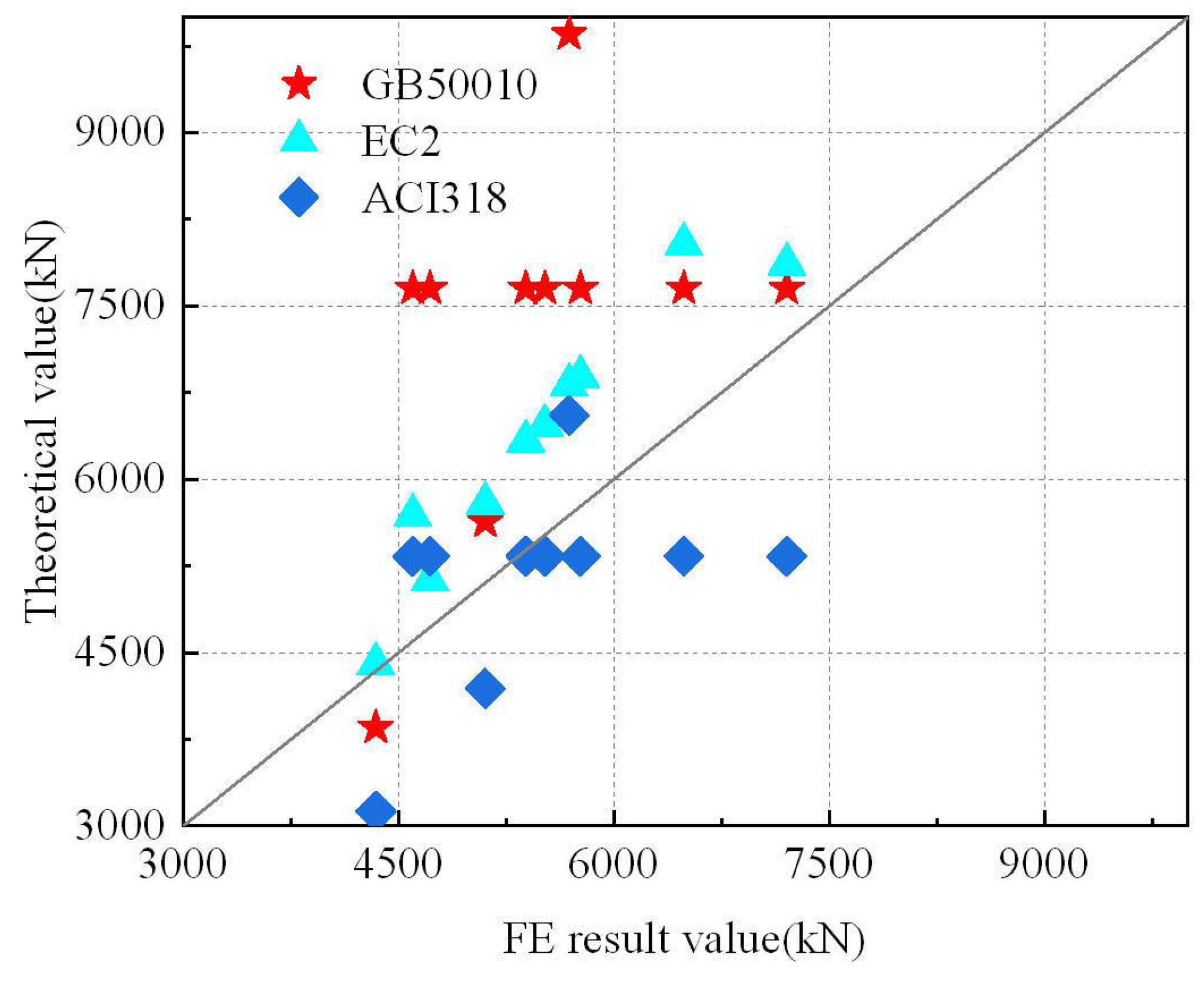
5.2. Evaluation of Design Codes

The punching shear resistances calculated by the equations in the design codes are compared against the FE results and shown in Figure 19. It can be seen that the predictions from the design codes are mostly higher the FE results, meaning the strength calculated by the design codes is unsafe. The calculation results of the equation used in EC2 [7] are most proximate to the FE results. This is because the flexure reinforcement ratio is considered in EC2 [7]. Overall, the calculation results predicted by GB50010 [1], EC2 [7] and ACI318 [8] may be inaccurate for the slab-column joints with a column cap.

6. Conclusions

FE models of the slab-column structures were developed to numerically analyse the effects of cap type and transverse stirrups on the structural behaviour of slab-column structures. The key findings are summarised as follows:

(1) The numerical results obtained from the FE simulation method were found to be consistent with the results obtained from the tests on slab-column structures. The FE simulation method was verified to be accurate and applicable;

(2) The slab-column joints with conventional caps are superior to their counterparts with reverse caps in terms of the load-carrying capacities, but they have lower ductility than their counterparts with reverse caps;

(3) The ultimate load of the slab-column joints with reverse cap can be increased by 2.4% by arranging transverse stirrups in column cap, but the ductility is decreased by 13.4%. For the slab-column joints with conventional cap, the ultimate load is decreased by 10.0% and the ductility is decreased by 1.6% when transverse stirrups are arranged in column cap;

(4) Therefore, when the design adopts the flat slab system with reverse column cap, arrangement of transverse stirrups in column cap should be determined based on the actual situation. When the design adopts the flat slab system with conventional column cap, it is not recommended to arrange transverse stirrups in column cap;

(5) The size and depth of the column cap can improve the bearing capacity of the slab-column joint, but the ductility of the slab-column joint will be reduced when the depth of the column cap is too large.

References

1. GB50010-2010 (2015); Code for Design of Concrete Structures. Ministry of Housing and Urban-Rural Development: Beijing, China, 2015.
2. Niehols, T.R. Statistical limitations upon the steel requirement in reinforced concrete flat slab floors. Soc. Civ. Eng. ASCE 1914, 77, 1670. [Google Scholar] [CrossRef]
3. Westergaard, H.M.; Slater, W.A. Moments and stresses in slabs. Proc. Am. Concr. Inst. 1921, 17, 415–538. [Google Scholar]
4. Elstner, R.C.; Hognestad, E. Shearing strength of reinforced concrete slabs. ACI J. 1956, 53, 29–58. [Google Scholar]
5. Regan, P.E. Design for punching shear. J. Struct. Eng. 1974, 52, 197–207. [Google Scholar]
6. Luo, Y.H.; Durrani, A.J. Equivalent beam model for flat- slab buildings. ACI Struct. J. 1995, 92, 115–124. [Google Scholar]
7. EC2 (2004); EN 1992-1-1:2004: Eurocode 2: Design of Concrete Structures—Part 1-1: General Rules and Rules for Buildings. National Standards Authority of Ireland: Dublin, Ireland, 2014.
8. ACI-318 (2019); Committee 318—Building Code Requirements for Structural Concrete (ACI 318-19) and Commentary on Building Code Requirements. American Concrete Institute: Farmington Hills, MI, USA, 2019.
9. Inácio, M.M.G.; Almeida, A.F.O.; Faria, D.M.V.; Lúcio, V.J.G.; Ramos, A.P. Punching of high strength concrete flat slabs without shear reinforcement. Eng. Struct. 2015, 103, 275–284. [Google Scholar] [CrossRef]
10. Majid, M.A.; Abdul, R.S.; Lee, S.C.; Ali, A.S. Numerical investigation of non-shear-reinforced UHPC hybrid flat slabs subject to punching shear. Eng. Struct. 2021, 241, 112444. [Google Scholar]
11. Genikomsou, A.S.; Polak, M.A. Finite element analysis of punching shear of concrete slabs using damaged plasticity model in ABAQUS. Eng. Struct. 2015, 98, 38–48. [Google Scholar] [CrossRef]
12. Balomenos, G.P.; Genikomsou, A.S.; Polak, M.A.; Pandey, M.D. Efficient method for probabilistic finite element analysis with application to reinforced concrete slabs. Eng. Struct. 2015, 103, 85–101. [Google Scholar] [CrossRef]
13. Wosatko, A.; Pamin, J.; Polak, M.A. Application of damage—Plasticity models in finite element analysis of punching shear. Comput. Struct. 2015, 151, 73–85. [Google Scholar] [CrossRef]
14. Jahangir, A.; Khan, M.A. FE Analysis on the effect of flexural steel on punching shear of slabs. Int. J. Eng. Res. Technol. 2013, 2, 2878–2901. [Google Scholar]
15. Elsamak, G.; Fayed, S. Parametric studies on punching shear behavior of RC flat slabs without shear reinforcement. Computers Concr. 2020, 25, 355–367. [Google Scholar]
16. Yooprasertchai, E.; Tiawilai, Y.; Wittayawanitchai, T.; Angsumalee, J.; Joyklad, P.; Hussain, Q. Effect of shape, number, and location of openings on punching shear capacity of flat slabs. Buildings 2021, 11, 484. [Google Scholar] [CrossRef]
17. Hussain, H.K.; Abbas, A.M.; Ojaimi, M.F. Fiber-type influence on the flexural behavior of RC two-way slabs with an opening. Buildings 2022, 12, 279. [Google Scholar] [CrossRef]
18. Mostofinejad, D.; Jafarian, N.; Naderi, A.; Mostofinejad, A.; Salehi, M. Effects of openings on the punching shear strength of reinforced concrete slabs. Structures 2020, 25, 760–773. [Google Scholar] [CrossRef]
19. Wu, L.; Huang, T.; Tong, Y.; Liang, S. A modified compression field theory based analytical model of RC slab-column joint without punching shear reinforcement. Buildings 2022, 12, 226. [Google Scholar] [CrossRef]
20. Ma, W. Behavior of Aged Reinforced Concrete Columns under High Sustained Concentric and Eccentric Loads. Ph.D. Dissertation, University of Nevada, Las Vegas, NV, USA, 2021. [Google Scholar]
21. Lin, Y.; Lin, F. Discussion on structural analysis and design of flat slab. Build. Struct. 2019, 49, 238–240. [Google Scholar]
22. Gong, M.; Lu, J. Design of flat slab with reverse column cap. Ind. Constr. 2011, 41, 233–235. [Google Scholar]
23. Simulia, D.S. Abaqus [Computer Software]; SIMULIA: Providence, RI, USA, 2016. [Google Scholar]
24. Sidiroff, F. Description of anisotropic damage application to elasticity. In Physical Non-Linearities in Structural Analysis; Springer: Berlin/Heidelberg, Germany, 1981; pp. 237–244. [Google Scholar]
25. Zhao, J. Study of Reinforced Concrete Bond-Slip Mechanism and Modelling Techniques under Cyclic Loading. Master’s Thesis, Chang’an University, Xi’an, China, 2016; p. 28. [Google Scholar]
26. Adetifa, B.; Polak, M.A. Retrofit of slab column interior connections using shear bolts. ACI Struct. J. 2005, 102, 268–274. [Google Scholar]
27. Park, R. State of the art report ductility evaluation from laboratory and analytical testing. In Proceedings of the Ninth World Conference on Earthquake Engineering, Tokyo, Japan, 2–9 August 1991. [Google Scholar]
28. JGJ/T 101-2015; Regulations for Seismic Testing of Buildings. Ministry of Housing and Urban-Rural Development: Beijing, China, 2015; p. 15.
29. Zhang, C.; Ma, W.; Liu, X.; Tian, Y.; Orton, S.L. Effects of high temperature on residual punching strength of slab-column connections after cooling and enhanced post-punching load resistance. Eng. Struct. 2019, 199, 109580. [Google Scholar] [CrossRef]
Figure 1. Stress–strain curve for concrete.
Buildings 12 01139 g001
Figure 2. Stress–strain curve of CDP model: (a) Compressive; (b) Tensile.
Buildings 12 01139 g002
Figure 3. Stress–strain curve of reinforcement.
Buildings 12 01139 g003
Figure 4. Specimen SB1 (dimensions in mm).
Buildings 12 01139 g004
Figure 5. FE model for Specimen SB1.
Buildings 12 01139 g005
Figure 6. Test and FE load–displacement curves of specimen SB1.
Buildings 12 01139 g006
Figure 7. Tensile side of concrete slab at failure.
Buildings 12 01139 g007
Figure 8. Specimen ZM01 (dimensions in mm).
Buildings 12 01139 g008
Figure 9. Reinforcement arrangements in specimens ZM01–ZM04 (dimensions in mm): (a) ZM01; (b) ZM02; (c) ZM03; (d) ZM04.
Buildings 12 01139 g009
Figure 10. FE model for specimen ZM01.
Buildings 12 01139 g010
Figure 11. FE load–displacement curves for specimens ZM01–ZM04. Note: Point A is yield point, Point B is ultimate point, and Point C is failure point.
Buildings 12 01139 g011
Figure 12. Selected positions of reinforcements: (a) ZM01 and ZM03; and (b) ZM02 and ZM04.
Buildings 12 01139 g012
Figure 13. Stress–displacement curves for reinforcements in each specimen in specimens ZM01–ZM04: (a) ZM01; (b) ZM02; (c) ZM03; and (d) ZM04.
Buildings 12 01139 g013aBuildings 12 01139 g013b
Figure 14. Tensile damage diagrams of tensile sides of specimens ZM01–ZM04 at yield load: (a) ZM01; (b) ZM02; (c) ZM03; and (d) ZM04.
Buildings 12 01139 g014aBuildings 12 01139 g014b
Figure 15. Tensile damage diagrams of tensile sides of specimens ZM01–ZM04 at ultimate load: (a) ZM01; (b) ZM02; (c) ZM03; and (d) ZM04.
Buildings 12 01139 g015
Figure 16. Tensile damage diagrams of tensile sides of specimens ZM01–ZM04 at failure load: (a) ZM01; (b) ZM02; (c) ZM03; and (d) ZM04.
Buildings 12 01139 g016aBuildings 12 01139 g016b
Figure 17. Influence of the size of column cap.
Buildings 12 01139 g017
Figure 18. Influence of the depth of column cap.
Buildings 12 01139 g018
Figure 19. Comparison of FE results with design codes.
Buildings 12 01139 g019