Choices of the Critical Frequency for φ in TL-φ Algorithms When Applied to Multi-Degree of Freedom Systems

Abstract

TL-$\phi$ algorithms are newly developed explicit structure-dependent integration algorithms utilized for solving the temporally discretized equations of motion. In contrast to the existing algorithms, the most significant improvement of TL-$\phi$ algorithms is in diminishing the amount of period errors by introducing a precorrection coefficient $\phi$ into the integration parameters of TL-$\phi$ algorithms, which is related to the critical frequency of a system. In the previous work, the fundamental frequency of the system is deemed to be the critical frequency, so that $\phi$ is a constant scaling corresponding to the fundamental frequency for both single-degree-of-freedom (SDOF) and multi-degree-of-freedom (MDOF) systems. However, for a MDOF system, the first mode may not contribute to the total response more than other ones under a given external excitation, calculating $\phi$ only by the fundamental frequency will underestimate the contribution of the higher-frequency modes to structural dynamics. In this paper, choices of the critical frequency for $\phi$ when applying TL-$\phi$ algorithms to MDOF systems are investigated thoroughly. By considering the initial structural properties of the system and the frequency characteristics of the external excitation simultaneously, a calculation criterion of $\phi$ for MDOF systems under specific external excitations is proposed. Four numerical examples with different initial structure properties and loading conditions are designed, and the results demonstrate that the proposed criterion can be potentially used to solve structural dynamic problems of MDOF systems with a more desirable numerical dispersion performance.

1. Introduction

Direct integration algorithms are widely utilized to solve temporally discretized equations of motion (EOMs) in the dynamic analysis of civil engineering structures [1,2,3]. Various integration algorithms have been well established based on different design conceptions in the past decades, such as the finite difference schemes [4,5,6,7], spectral methods of discretization [8,9], and methods based on other ideas [10,11,12]. In general, integration algorithms can be classified as explicit and implicit according to the expressions of displacement and velocity. An algorithm is explicit if the displacement and velocity at the current time step can be expressed in terms of all the known responses at the previous time steps [13], otherwise it is implicit. Explicit algorithms are preferred over implicit ones since they do not involve nonlinear iterations during a step-by-step simulation and possess favorable efficiencies for long-time simulations with small time steps. However, conditional stability of the most explicit algorithms limits their applications in solving dynamic problems, which leads to a time-step size restriction especially for a multi-degree-of-freedom (MDOF) system with high natural frequencies [14]. Hence, integration algorithms that possess both explicit expressions and unconditional stability deserve more attention.

Recently, a new family of integration algorithms classified as structure-dependent integration methods (SDIM) have been well developed and widely used in structural dynamics. In contrast to a structure-independent integration method (SIIM) whose integration parameters of the difference equations are constant, parameters in an SDIM are determined by the initial structural properties, including structural natural frequency, damping ratio and selected time steps [15]. The first SDIM was developed by Chang [16] (named Chang algorithm) for pseudodynamic testing, and is unconditionally stable for linear systems and possesses second-order accuracy. However, this method is semi-explicit as the displacement increment is explicit in form while that of the velocity is implicit. Then, Chen [17] proposed a new SDIM (named CR algorithm) which has explicit expressions for both the displacement and velocity increments. The CR algorithm also demonstrates favorable performance such as unconditional stability for linear systems and second-order accuracy. Rezaiee [18] developed a new algorithm called the USE algorithm. In this method, the expressions of the displacement and velocity increments are defined in terms of the accelerations of the two previous time steps and three integration parameters were introduced to control the stability and numerical dissipation of procedure. Tang [19] presented another type of explicit SDIM known as the Real-time Substructure Testing algorithm (referred to as TL algorithm in this paper), in which the two structure-dependent integration parameters are introduced only in the displacement increment. It is noted that the TL algorithm is unconditionally stable for linear systems and also bears second-order accuracy [20].

The numerical properties of an SDIM are typically evaluated by its stability and accuracy. In order to achieve higher stability limits, many improvements have been conducted for nonlinear systems [21,22,23]. Energy dissipation and numerical dispersion are two important indexes for evaluating the accuracy of an algorithm, which can be measured by amplitude decay (AM) and period elongation (PE) in the time domain. Some researchers [24,25,26,27,28] have developed various families of algorithms that can control the amount of energy dissipation by introducing different control parameters in the integration parameters. Few researchers work on the issue of numerical dispersion of integration algorithms. Li [29] proposed a new method of reducing PE (or numerical dispersion) by introducing a parameter that is weighted by the mass matrix and stiffness matrix into the original algorithm. As only the mass matrix of the system is changed slightly, the convergence rate and stability property of the algorithm are maintained. Tang and Ren [30] presented a new family of explicit SDIM with controllable numerical dispersion based on the TL algorithm, known as TL-$\phi$ algorithms. By introducing a scaling parameter $\phi$ into the two integration parameters of TL algorithm, the values of PE at a certain structural natural frequency can be greatly diminished when compared to other well-developed algorithms.

In TL-$\phi$ algorithms, $\phi$ is a precorrection coefficient that is equal to the ratio of the frequency (${\omega }_D$) in the discrete domain to the one (${\omega }_A$) in the continuous domain. This reveals the degree of frequency distortion during the discretization of a continuous system, and introduction of $\phi$ in the mapping rules of the discretization will ensure consistency between ${\omega }_D$ and ${\omega }_A$ in numerical characteristics. For an MDOF system, the calculation of $\phi$ depends on the critical frequency ${\omega }_c={\omega }_A$ that dominates the total responses of the original continuous system. In the previous work [30], the fundamental frequency ${\omega }_1$ is regarded as ${\omega }_c$, so that $\phi$ becomes a constant scaling for all the modes of the system when calculating the integration parameters of the TL-$\phi$ algorithms. However, the first mode may not uniquely contribute to the dynamic responses of an MDOF system under a given external excitation, and the determination of ${\omega }_c$ should take the numerical properties of both the original system and external excitation into consideration. In this study, choices of ${\omega }_c$ for $\phi$ when applying TL-$\phi$ algorithms to MDOF systems are thoroughly investigated. Two factors that control the relative importance of any mode in the total dynamic responses are introduced to consider the effect of the initial structural properties of the system and the frequency characteristics of the external excitation on the determination of ${\omega }_c$ simultaneously. Then, the selection criterion of ${\omega }_c$ for systems subjected to harmonic excitation and seismic waves are proposed, respectively, and studied with respect to the accuracy and efficiency.

2. Formulation of TL-$\mathit{\phi }$ Algorithms for MDOF Systems

The formulation of TL-$\phi$ algorithms for an N-DOF system can be expressed in discrete form as [30]

$$\mathbf{M}{\ddot{\mathbf{U}}}_{i+1}+\mathbf{C}{\dot{\mathbf{U}}}_{i+1}+\mathbf{K}{\mathbf{U}}_{i+1}={\mathbf{F}}_{i+1}$$

(1)

$${\mathbf{U}}_{i+1}={\mathbf{U}}_i+{\alpha }_1\Delta t{\dot{\mathbf{U}}}_i+{\alpha }_2\Delta t^2{\ddot{\mathbf{U}}}_i$$

(2)

$${\dot{\mathbf{U}}}_{i+1}={\dot{\mathbf{U}}}_i+\Delta t{\ddot{\mathbf{U}}}_i$$

(3)

where, $\mathbf{M}$, $\mathbf{C}$ and $\mathbf{K}$ are the mass, viscous damping and stiffness matrix, $N\times N$, respectively; $\ddot{\mathbf{U}}$, $\dot{\mathbf{U}}$ and $\mathbf{U}$ are the acceleration, velocity, and displacement vector, $N\times 1$, respectively; $\mathbf{F}$ is the external force vector, $N\times 1$; ${\alpha }_1$ and ${\alpha }_2$ are the integration parameter matrices, $N\times N$, which are

$$\left\{\begin{array}{c}{\alpha }_1=4{\mathbf{B}}^{-1}·\mathbf{M}\hfill \\ {\alpha }_2={\mathbf{B}}^{-1}·(4\mathbf{M}-\Delta t\mathbf{C}-2\mathit{\phi }·\mathbf{D}+\mathbf{E})\hfill \end{array}\right.$$

(4)

where, $\mathbf{B}=4{\mathit{\phi }}^2·\mathbf{M}+2\Delta t\mathit{\phi }·\mathbf{C}+\Delta t^2·\mathbf{K}$; $\mathbf{D}={\left({\mathsf{\Phi }}^T\right)}^{-1}·{\mathbf{D}}^{*2}·{\mathsf{\Phi }}^{-1}$; $\mathbf{E}={\left({\mathsf{\Phi }}^T\right)}^{-1}·{\mathbf{E}}^{*}·{\mathsf{\Phi }}^{-1}$; $\mathit{\phi }=\mathrm{diag}[{\phi }_1,\cdots {\phi }_j,\cdots ,{\phi }_N]$, and

$${\phi }_j=\frac{\arctan \left({\mathsf{\Omega }}_j/2\right)}{{\mathsf{\Omega }}_j/2}j=1,2,...,N$$

(5)

in which, ${\mathsf{\Omega }}_j={\omega }_j\Delta t$, ${\omega }_j$ is the natural frequency of the jth mode, and $\Delta t$ is the time step selected for integrating.

3. Frequency Response under Arbitrary Excitation

Based on the mode-superposition method, the dynamic response of a linear MDOF system can be obtained by solving separately for that of each mode and then superposing these modes to obtain the total response in the original geometric coordinates. Thus, the numerical characteristics of an algorithm applied in an MDOF system can be evaluated for each mode in the same way as for a single-degree-of-freedom (SDOF) system. The numerical characteristics of TL-$\phi$ algorithms under the free-vibration response have been fully investigated in the previous work [30]. This section focuses on the frequency response of TL-$\phi$ algorithms under arbitrary excitation with initial conditions of $x_0=0$ and ${\dot{x}}_0=0$. For any arbitrary mode n, the equation of motion of an SDOF system under external excitation is

$$\begin{gathered} {\ddot{y}}_n\left(t\right)+2{\xi }_n{\omega }_n{\dot{y}}_n\left(t\right)+{\omega }_n^2{y}_n\left(t\right)=\frac{f_n\left(t\right)}{m_n}n=1,2,\cdots ,N \\ {\xi }_n=\frac{c_n}{2m_n{\omega }_n},{\omega }_n=\sqrt{\frac{k_n}{m_n}} \end{gathered}$$

(6)

where, $m_n={\mathit{\varphi }}_n^{\mathrm{T}}\mathbf{M}{\mathit{\varphi }}_n$, $c_n={\mathit{\varphi }}_n^{\mathrm{T}}\mathbf{C}{\mathit{\varphi }}_n$ and $k_n={\mathit{\varphi }}_n^{\mathrm{T}}\mathbf{K}{\varphi }_n$ are modal mass, modal damping and modal stiffness for the nth mode, respectively; ${\ddot{y}}_n$, ${\dot{y}}_n$ and $y_n$ are acceleration, velocity, and displacement for the nth mode, respectively; ${\xi }_n$ and ${\omega }_n$ are the natural frequency and viscous damping ratio for the nth mode, respectively; $f_n={\mathit{\varphi }}_n^{\mathrm{T}}\mathbf{F}\left(t\right)$ is modal force for the nth mode. For simplicity, the subscript n will be omitted from this point onward.

The continuous transfer function $G\left(s\right)$ that relates the force $f\left(t\right)$ to the displacement $y\left(t\right)$ is given by

$$G\left(s\right)=\frac{Y\left(s\right)}{F\left(s\right)}=\frac{1}{m(s^2+2\xi \omega +{\omega }^2)}$$

(7)

where, $Y\left(s\right)$ and $F\left(s\right)$ are the Laplace transforms of $y\left(t\right)$ and $f\left(t\right)$, respectively, and s is the Laplace transform parameter.

Substituting $s=i\tilde{\omega }$ into Equation (7), the complex frequency response function of the steady-state response under the harmonic excitation of $f\left(t\right)=f_0{e}^{i\tilde{\omega }t}$ can be determined by

$$G\left(i\tilde{\omega }\right)=\frac{Y\left(i\tilde{\omega }\right)}{F\left(i\tilde{\omega }\right)}=\frac{f_0}{k[(1-{\beta }^2)+i\left(2\xi \beta \right)]},\beta =\tilde{\omega }/\omega$$

(8)

in which, $\beta$ is frequency ratio, that is, the ratio of the excitation frequency $\tilde{\omega }$ to the modal frequency $\omega$. The dynamic magnification factor (DMF) D and phase $\theta$ of $G\left(i\tilde{\omega }\right)$ are

$$D=\frac{G\left(i\tilde{\omega }\right)}{y_{\mathrm{st}}}=\frac{1}{\sqrt{{(1-{\beta }^2)}^2+{\left(2\xi \beta \right)}^2}}$$

(9)

$$\theta ={\tan }^{-1}\left(\frac{2\xi \beta }{1-{\beta }^2}\right)$$

(10)

where $y_{\mathrm{st}}=f_0/k$ is the displacement which would be produced by the load $f_0$ applied statically. The two factors, D and $\theta$, calculated by Equations (9) and (10) denote the exact dynamic magnification factor and phase, respectively.

Similarly, the complex frequency response function for TL-$\phi$ algorithms in the discrete domain can be obtained by introducing $z=e^{i\tilde{\omega }\Delta t}$ into the discrete transfer function $G\left(z\right)$, which is

$$G\left(z\right)=\frac{Y\left(z\right)}{F\left(z\right)}=\frac{{\alpha }_2\Delta t^{2}z+({\alpha }_1-{\alpha }_2)\Delta t^2}{m{z}^2+m({\alpha }_2{\mathsf{\Omega }}^2+2\xi \mathsf{\Omega }-2)z+m[({\alpha }_1-{\alpha }_2){\mathsf{\Omega }}^2-2\xi \mathsf{\Omega }+1]}$$

(11)

and the numerical DMF and phase are expressed as $D_{\mathrm{num}}=kG\left(e^{i\tilde{\omega }\Delta t}\right)$ and ${\theta }_{\mathrm{num}}=\angle G\left(e^{i\tilde{\omega }\Delta t}\right)$, respectively.

Figure 1 shows $D_{\mathrm{num}}$ and ${\theta }_{\mathrm{num}}$ for TL-$\phi$ algorithms when compared to the exact solution of D and $\theta$. The damping ratio $\xi$ is taken as 0.1, while the different values of $\mathsf{\Omega }=$ 0.2, 1.0 and 2.0 are considered and the corresponding coefficients $\phi$ become 0.9967, 0.9273 and 0.7854, respectively. Meanwhile, $D_{\mathrm{num}}$ and ${\theta }_{\mathrm{num}}$ for the other three well-developed explicit integration algorithms, including Chang algorithm, CR algorithm and TL algorithm, are also calculated and shown in each sub-figure.

It can be seen in Figure 1a that $D_{\mathrm{num}}$ and ${\theta }_{\mathrm{num}}$ for all the integration algorithms agree well with their accurate counterparts when $\mathsf{\Omega }=0.2$. For a larger value of $\mathsf{\Omega }=$ 1.0 and 2.0, the numerical resonance peak shifts to the left for all the algorithms, and the larger the value of $\mathsf{\Omega }$, the further left the numerical resonance peak shifts. It is also observed that the left-shift values of the numerical resonance peak of TL-$\phi$ algorithms are smaller than those of other algorithms, indicating a smaller PE in the numerical solution. This property conforms to the findings presented in previous work [30]. In addition, the maximum values of $D_{\mathrm{num}}$ for all the algorithms become larger with an increasing value of $\mathsf{\Omega }$ than those of the exact solution.

4. Critical Frequency Selection for $\mathit{\phi }$ in TL-$\mathit{\phi }$ Algorithms

When applying TL-$\phi$ algorithms to a MDOF system, the first and most important issue is the calculation of $\mathit{\phi }$. Precorrection for each mode of the system may possess high accuracy but is time consuming, especially when the number of DOFs is huge. It is quite promising that determination of a critical frequency ${\omega }_c$ for $\mathit{\phi }$, reduces $\mathit{\phi }$ to a constant scaling for all the modes.

In general, the first mode of an MDOF system possesses a dominant impact on the total responses of free-vibration and forced-vibration under specific external excitation, such as an earthquake tends to excite the response of a structure mainly in its first mode [31]. However, higher modes of an MDOF system may contribute more to the response than the first one, and the determination of ${\omega }_c$ should consider both the initial structural properties of the system and the frequency characteristics of the external excitation. It should be noted that the importance of any mode in the total dynamic response depends on two factors: (1) The DMF that depends on the frequency ratio of the external excitation to the mode, as discussed in the previous section; (2) the modal participation factor (MPF) that is determined by the interaction of the mode shape with the spatial distribution of the external excitation.

4.1. Determination of ${\omega }_c$ Based on DMF

According to the frequency response analysis, the maximum response amplitude occurs at a frequency ratio $\beta$ approaching close to (slightly less than) unity, i.e., the external excitation frequency approaches a certain modal frequency, known as resonance. For an MDOF system, an arbitrary external excitation will excite the resonance response of any mode, and the determination of ${\omega }_c$ should consider ${\beta }_i$ that relates the excitation frequency $\tilde{\omega }$ to the ith mode frequency ${\omega }_i$.

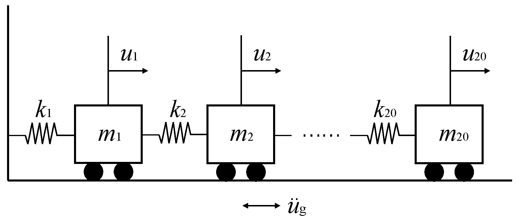
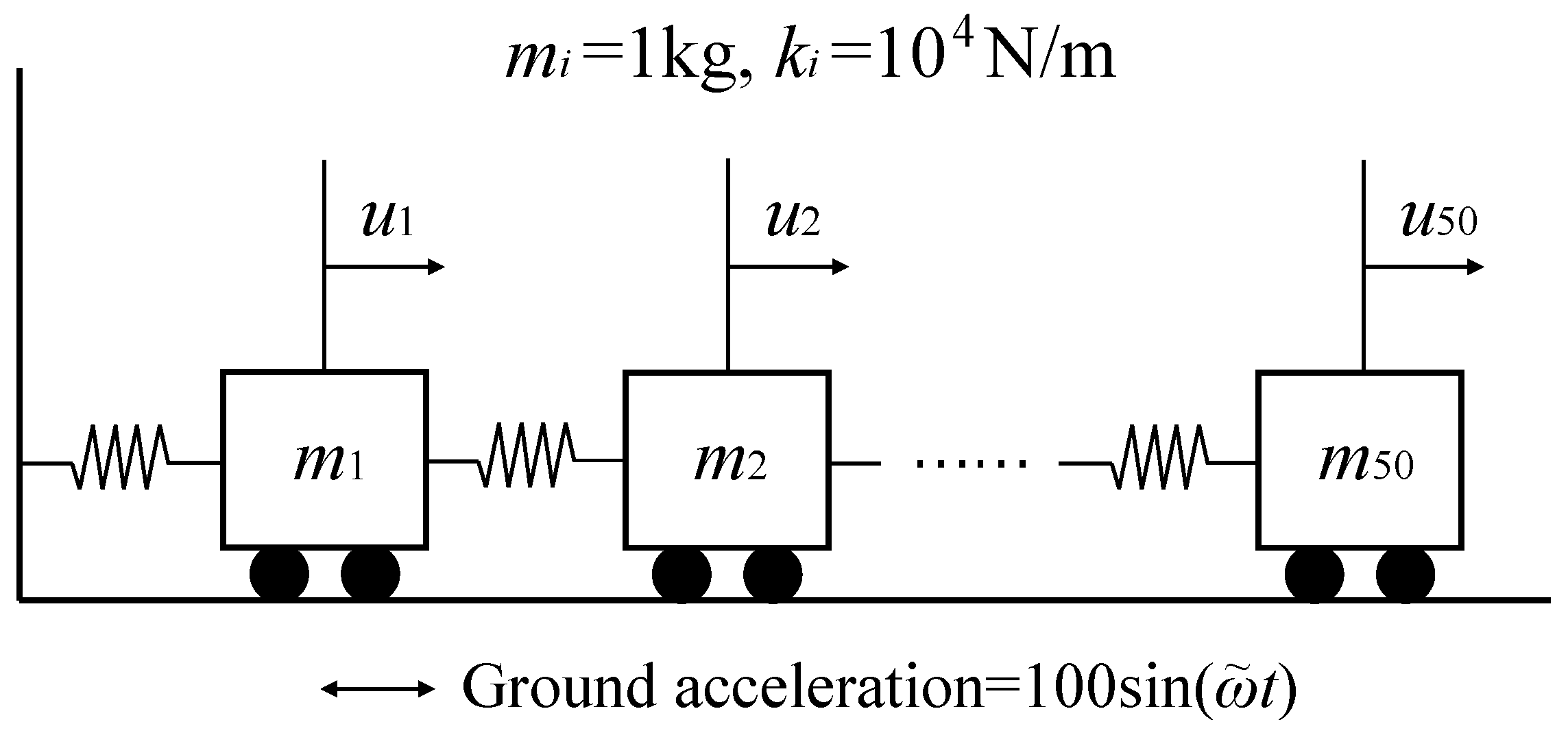
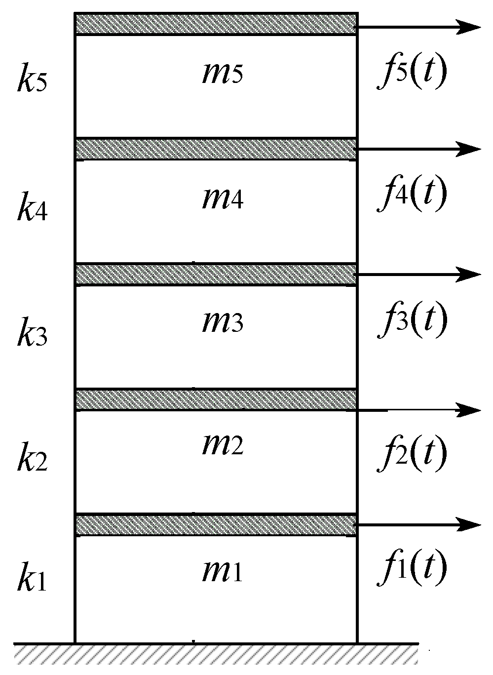
In this section, a spring-mass system with 20-DOF is set up to investigate the relationship between ${\omega }_c$ and $\tilde{\omega }$, as shown in Figure 2. A total of 12 models with different structural properties are intentionally designed, and the fundamental frequencies of each model are shown in

Table 1. The fundamental frequencies of the models ($\mathrm{rad}/\mathrm{s}$).

Model	1	2	3	4	5	6
${\omega }_1$	0.0699	0.2047	0.4423	0.7661	1.0834	1.7129
Model	7	8	9	10	11	12
${\omega }_1$	2.4225	3.4259	5.4168	7.6605	12.112	19.779

. The system is assumed to be linear elastic and is subjected to a ground acceleration ${\ddot{u}}_g\left(t\right)$ of sine-wave form as follows,

$${\ddot{u}}_g\left(t\right)=\sin \left(\tilde{\omega }t\right)$$

(12)

and then, ${\mathbf{F}}_{i+1}$ in Equation (1) is expressed as

$${\mathbf{F}}_{i+1}=\mathbf{M}\mathbf{I}·{\ddot{u}}_g^{i+1}$$

(13)

TL-$\phi$ algorithms with ${\omega }_c=1,1.5,2,2.5,3,4,5,6,7,8,9,10,11,12$ for $\phi$ are applied to calculate the displacement responses of the system under the harmonic excitation with $\tilde{\omega }=1,1.5,2,3,4,5,6,7,8,9,10$, respectively. One error indicator, normalized root-mean-square error (NRMSE) that is sensitive to frequency differences of the dynamic responses, is adopted for accuracy analysis and defined as

$$\mathrm{NRMSE}=\frac{\sqrt{{\sum }_{i=1}^m\frac{{(u_{\mathrm{ES},i}-u_{\mathrm{NS},i})}^2}{m}}}{max\left(u_{\mathrm{NS},i}\right)-min\left(u_{\mathrm{NS},i}\right)}$$

(14)

where, u is the displacement of $m_{20}$; subscript NS and ES represent the numerical solution obtained by TL-$\phi$ algorithms and exact solution derived from the mode-superposition method, respectively; $m=t/\Delta t$ is the number of the samples, where t is the duration of the external excitation and $\Delta t=0.01$ s is the time step for numerical simulations.

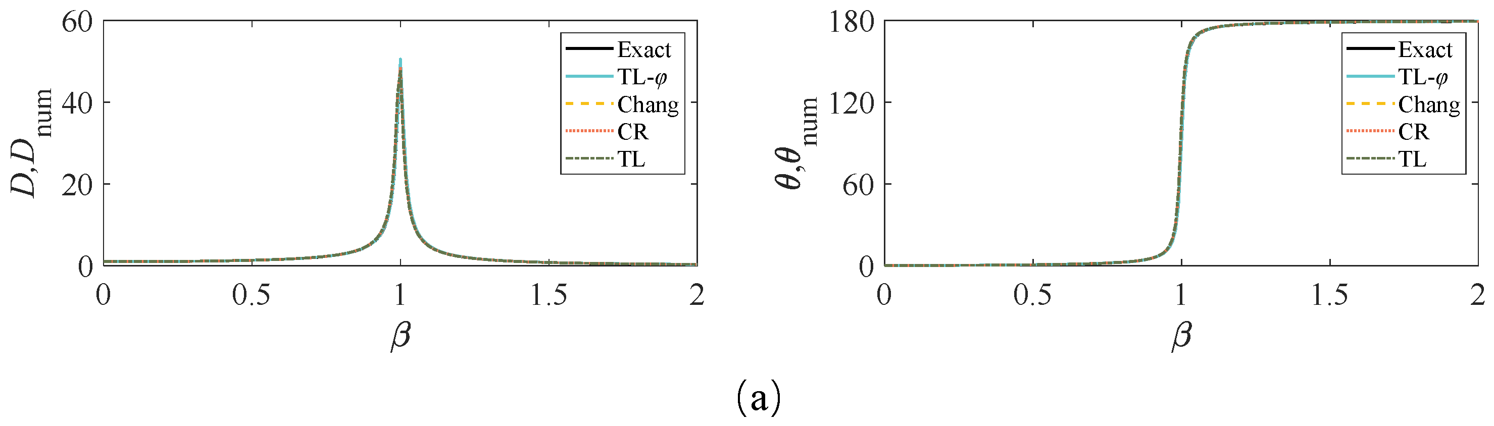
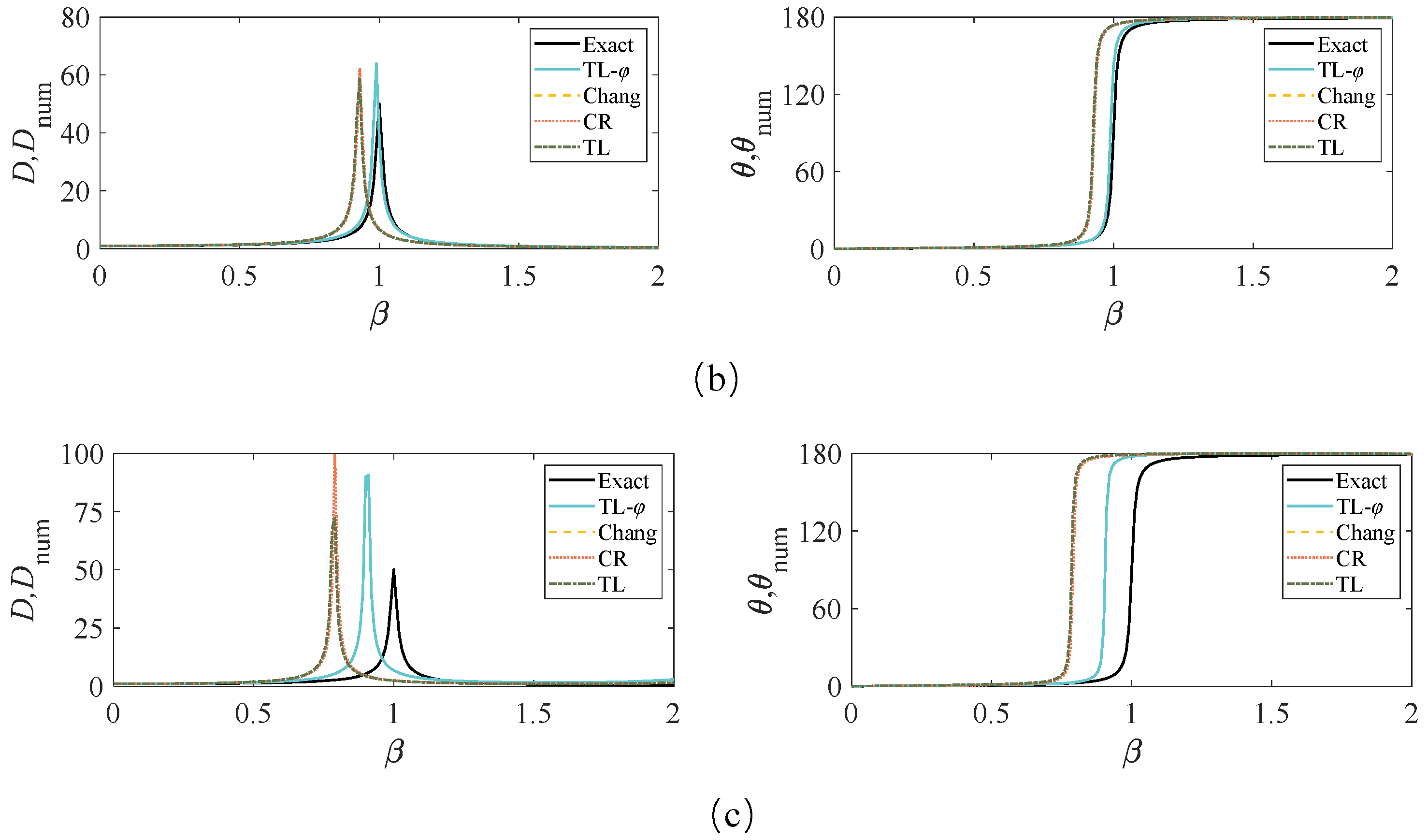
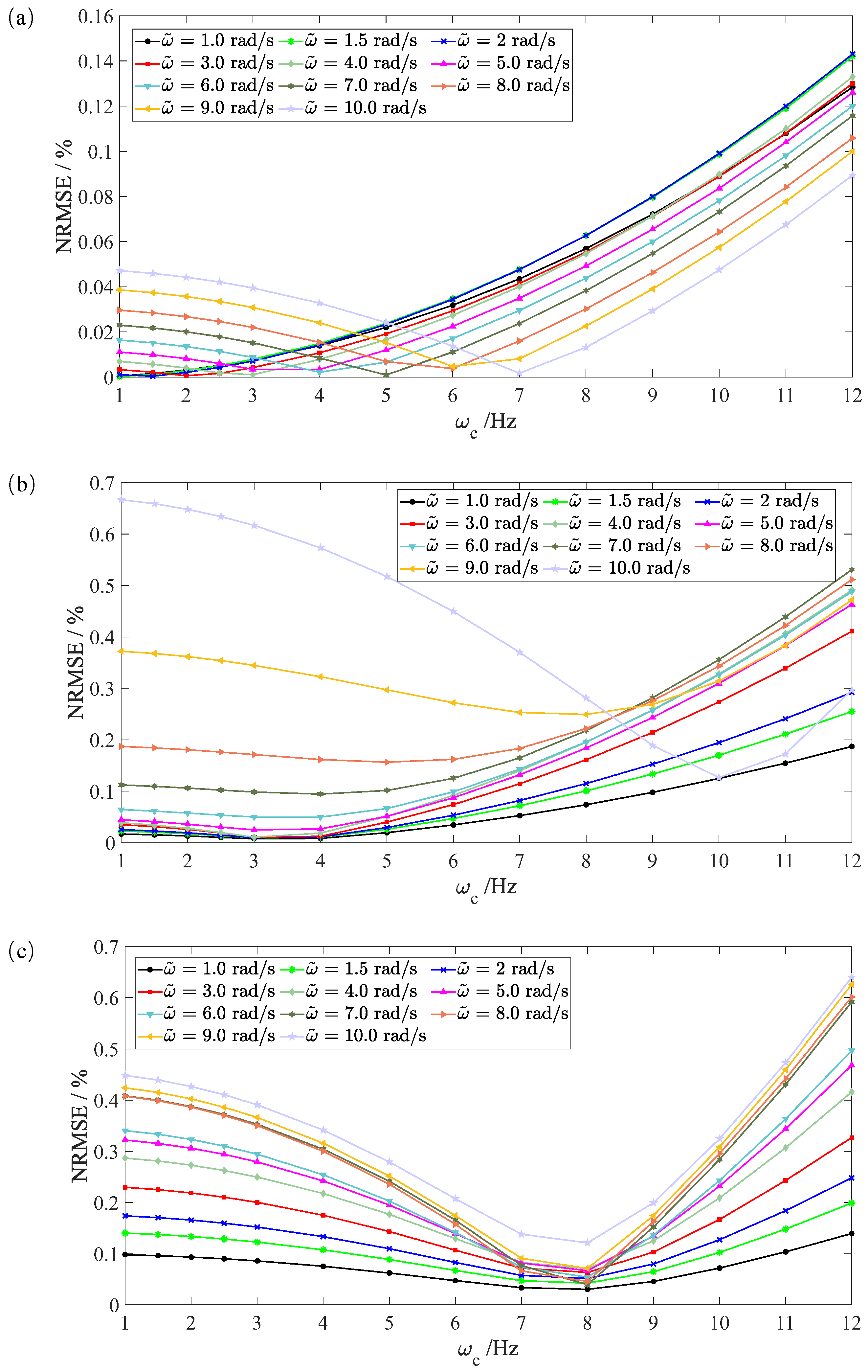
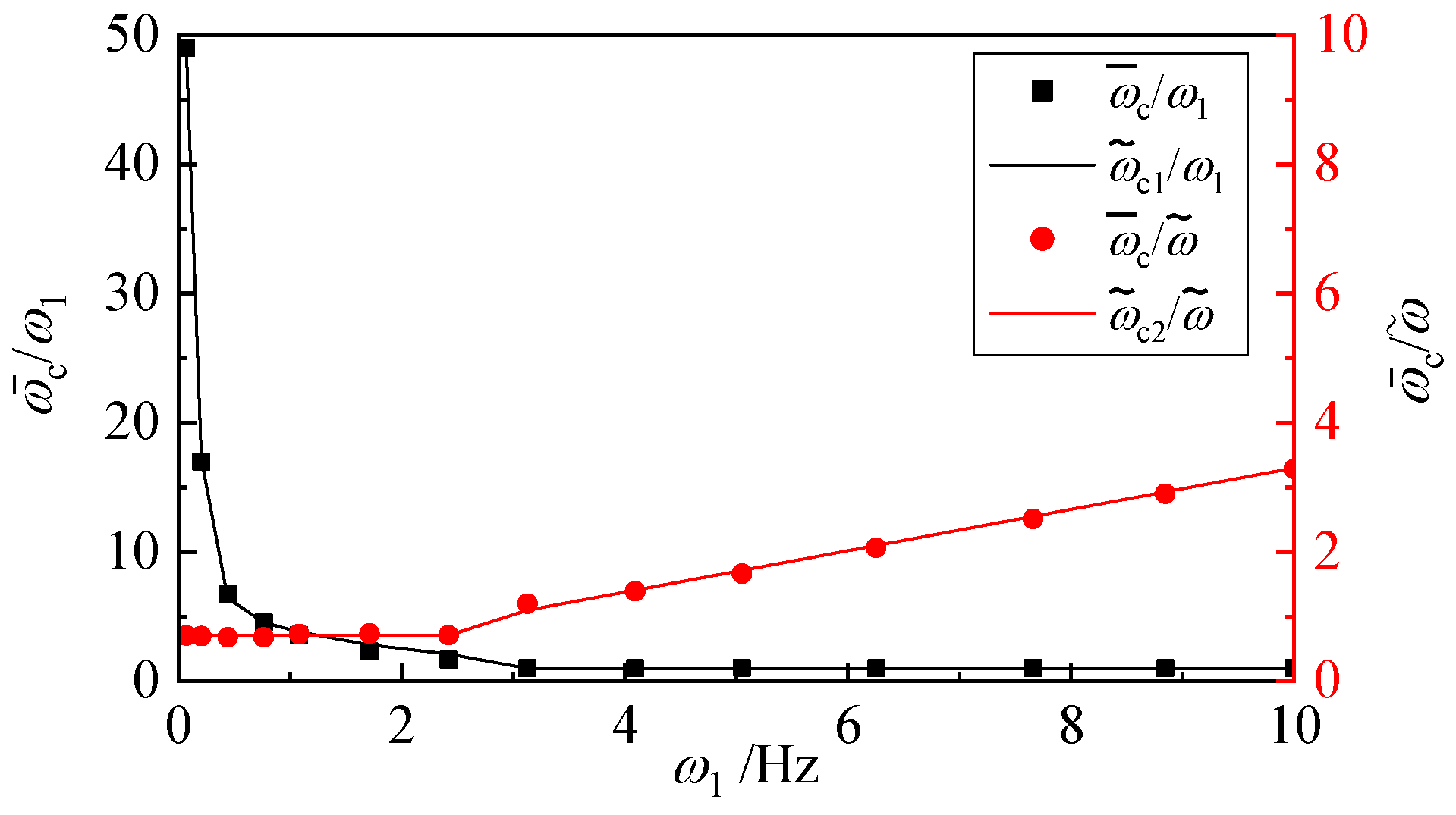
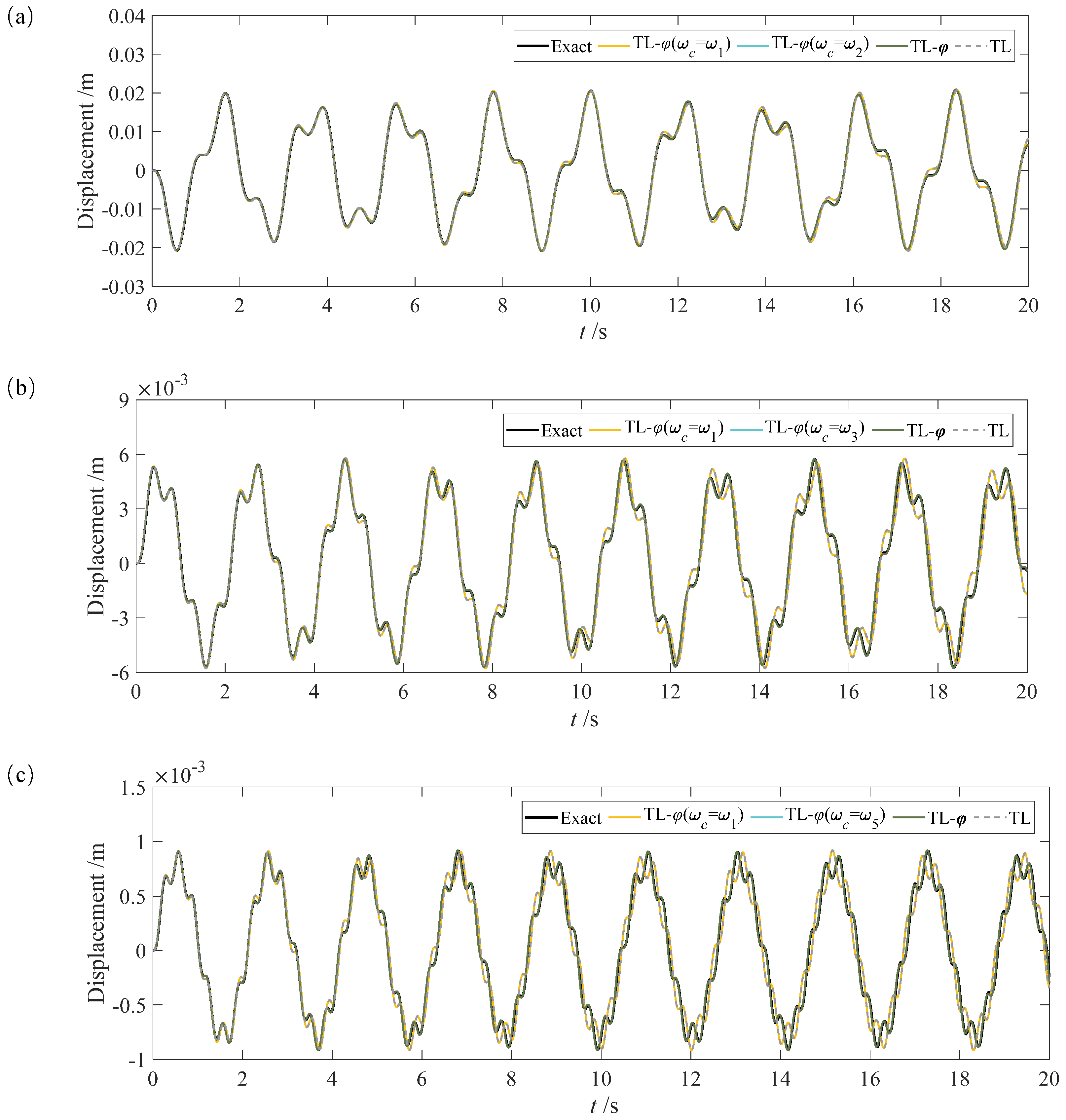
Plotted in Figure 3a–c are the variations of NRMSE with the increasing of ${\omega }_c$ for models 1, 8 and 10, and similar curves can be obtained for the rest of the models. It can be seen that the NRMSE is minimal at: (1) ${\omega }_c={\omega }_1$ when ${\beta }_1<1$, i.e., $\tilde{\omega }<{\omega }_1$; (2) ${\omega }_c={\omega }_i$ when ${\beta }_i\approx 1$, i.e., $\tilde{\omega }\approx {\omega }_i(i=1,2,...,10)$; (3) otherwise, ${\omega }_c$ is between values of ${\omega }_1$ and $\tilde{\omega }$, which verifies the importance of ${\omega }_1$ and $\tilde{\omega }$ in determining ${\omega }_c$ for the calculation of $\phi$ in TL-$\phi$ algorithm. In order to determine the value of ${\omega }_c$ in (3), more numerical models with different values of ${\omega }_1$ (less than 10 Hz) are designed to calculate the optimal critical frequencies ${\widehat{\omega }}_c$ that correspond to the minimal NRMSE. To diminish the effect of the fundamental frequency randomly selected for numerical simulation on fitting results, arithmetic mean values of ${\widehat{\omega }}_c$ for each model are calculated according to the following formula,

$$\frac{{\overline{\omega }}_c}{{\omega }_1}=\frac{1}{n}\sum \frac{{\widehat{\omega }}_c}{{\omega }_1},\frac{{\overline{\omega }}_c}{\tilde{\omega }}=\frac{1}{n}\sum \frac{{\widehat{\omega }}_c}{\tilde{\omega }}$$

(15)

in which, n is the number of the harmonic excitation $\tilde{\omega }$.

Table 2. Ratios of the average values of ${\overline{\omega }}_c$ to ${\omega }_1$ and $\tilde{\omega }$.

Model	1	2	3	4	5	6	7
${\omega }_1$$/\mathrm{rad}/\mathrm{s}$	0.0699	0.2047	0.4423	0.7661	1.0834	1.7129	2.4225
${\overline{\omega }}_c/{\omega }_1$	49.947	16.984	6.7213	4.5392	3.5496	2.3007	1.6587
${\overline{\omega }}_c/\tilde{\omega }$	0.7072	0.6997	0.6805	0.6785	0.7325	0.7398	0.7123
Model	8	9	10	11	12	13	14
${\omega }_1$$/\mathrm{rad}/\mathrm{s}$	3.1274	4.0947	5.0512	6.2548	7.6606	8.8456	9.9986
${\overline{\omega }}_c/{\omega }_1$	1.0000	1.0000	1.0241	1.0072	1.0034	1.0028	1.0039
${\overline{\omega }}_c/\tilde{\omega }$	1.2005	1.3948	1.6646	2.0673	2.5153	2.9031	3.2833

lists the ratio of the mean values of ${\overline{\omega }}_c$ to ${\omega }_1$ and $\tilde{\omega }$ for the 15 models. Figure 4 shows the scatter diagram of mean values varying with ${\omega }_1$, which indicates that ${\overline{\omega }}_c/{\omega }_1$ decay exponentially with an increasing of ${\omega }_1$, while ${\overline{\omega }}_c/\tilde{\omega }$ increases linearly with an increasing of ${\omega }_1$. According to these rules, a regression analysis is conducted and the fitting formulas are

$$\begin{array}{c}\hfill \begin{array}{c}\hfill \frac{{\tilde{\omega }}_{c1}}{{\omega }_1}=\left\{\begin{array}{cc}1+86e^{-10.7{\omega }_1}+7.8e^{-1.04{\omega }_1},\hfill & 0<{\omega }_1<3\hfill \\ 1,\hfill & {\omega }_1\ge 3\hfill \end{array}\right.\end{array}\end{array}$$

(16)

$$\begin{array}{c}\hfill \begin{array}{c}\hfill \frac{{\tilde{\omega }}_{c2}}{\tilde{\omega }}=\left\{\begin{array}{cc}0.71,\hfill & 0<{\omega }_1<2.5\hfill \\ 0.32{\omega }_1+0.1,\hfill & {\omega }_1\ge 2.5\hfill \end{array}\right.\end{array}\end{array}$$

(17)

$$\begin{array}{c}\hfill \begin{array}{c}\hfill {\tilde{\omega }}_c=\left\{\begin{array}{cc}{\tilde{\omega }}_{c1},\hfill & \frac{{\tilde{\omega }}_{c1}}{{\omega }_1}\le \frac{{\tilde{\omega }}_{c2}}{\tilde{\omega }}\hfill \\ {\tilde{\omega }}_{c2},\hfill & \frac{{\tilde{\omega }}_{c1}}{{\omega }_1}>\frac{{\tilde{\omega }}_{c2}}{\tilde{\omega }}\hfill \end{array}\right.\end{array}\end{array}$$

(18)

where, ${\tilde{\omega }}_{c1}$ and ${\tilde{\omega }}_{c2}$ are predicted values of ${\overline{\omega }}_c$ in Equation (15). The smaller one of the two radios derived from Equations (16) and (17) is considered to calculate ${\tilde{\omega }}_c$. Then, the criterion of determining ${\omega }_c$ for the calculation of $\phi$ in TL-$\phi$ algorithm when applied to MDOF systems can be expressed as

$$\begin{array}{c}\hfill \begin{array}{c}\hfill {\omega }_c=\left\{\begin{array}{cc}{\omega }_1,\hfill & {\beta }_1<1\hfill \\ {\omega }_i,\hfill & {\beta }_i=1\pm 0.1\hfill \\ {\tilde{\omega }}_c,\hfill & \mathrm{otherwise}\hfill \end{array}\right.\end{array}\end{array}$$

(19)

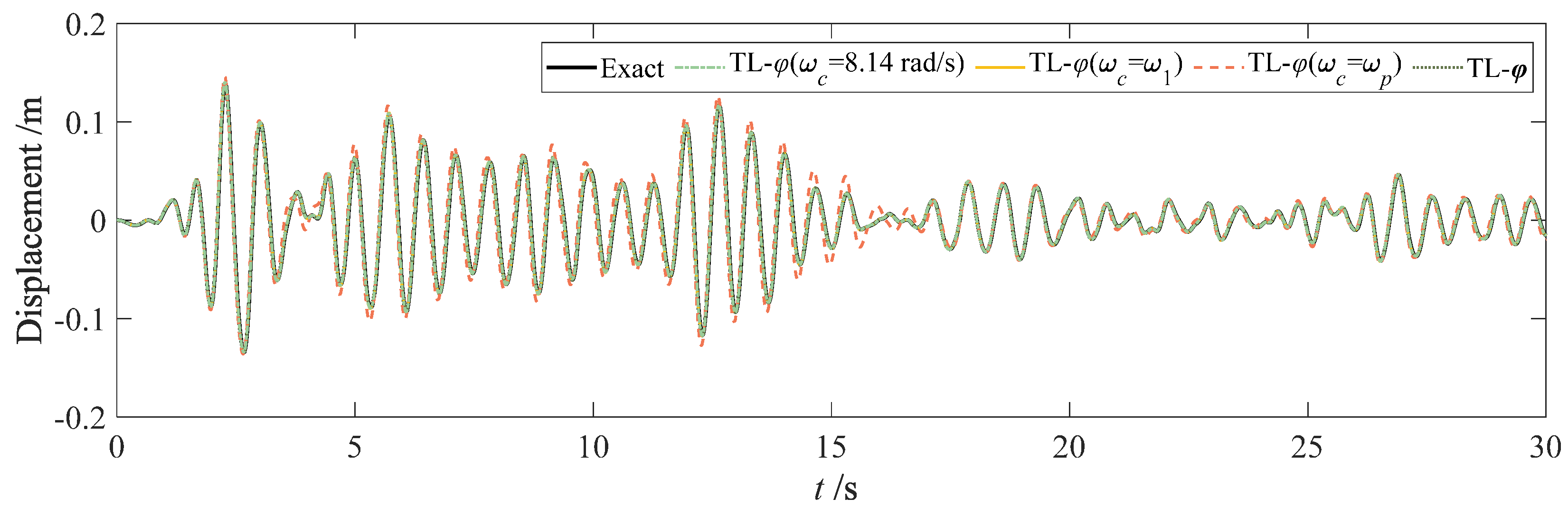
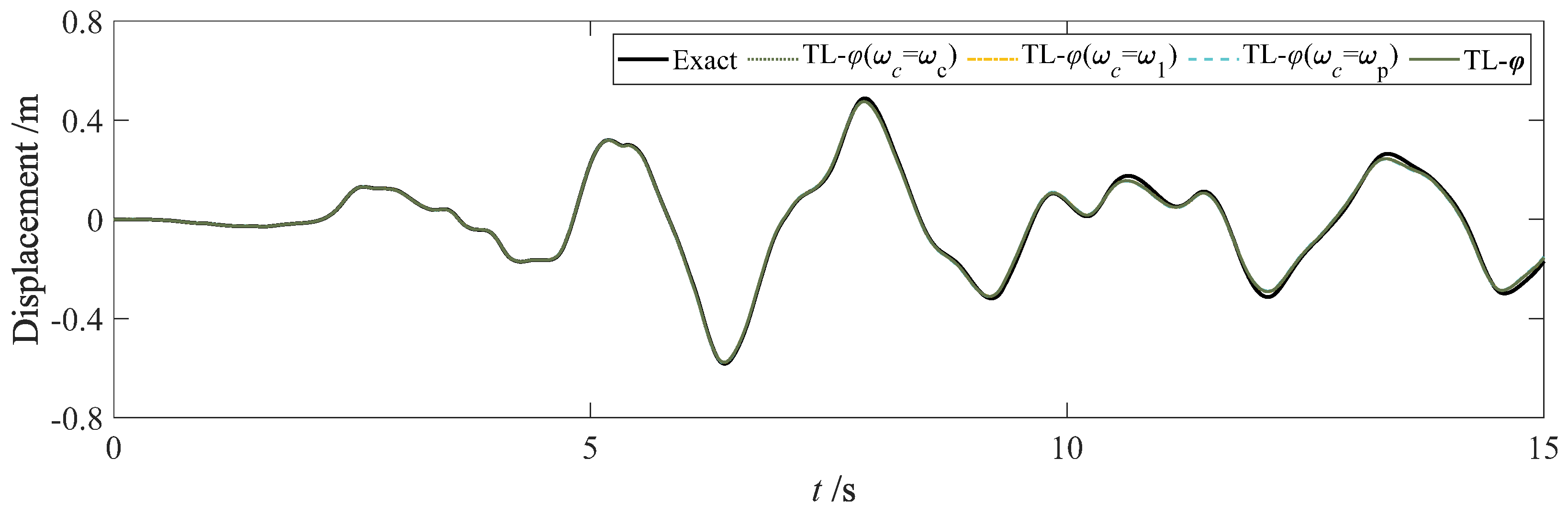
When an MDOF system is subjected to an earthquake, ${\ddot{u}}_g\left(t\right)$ in Equation (12) represents a practical seismic record. It is known that the contribution of the first mode to the dynamic responses of the system is much greater than that of the other higher-order modes when the fundamental frequency of the system is close to or higher than the main frequency component of a seismic motion. In addition, defining ${\omega }_c={\omega }_1$ will achieve relatively high accuracy of the dynamic responses. However, the effect of the high-order modes on structural dynamics cannot be ignored when the fundamental frequency of the system is lower than the main frequency component of a seismic motion. Thus, it is of great interest to examine the influence of the spectral characteristic of a seismic motion on the determination of ${\omega }_c$. Then, $\tilde{\omega }$ will be replaced by the peak frequency of the response spectrum ${\omega }_p$ in the following.

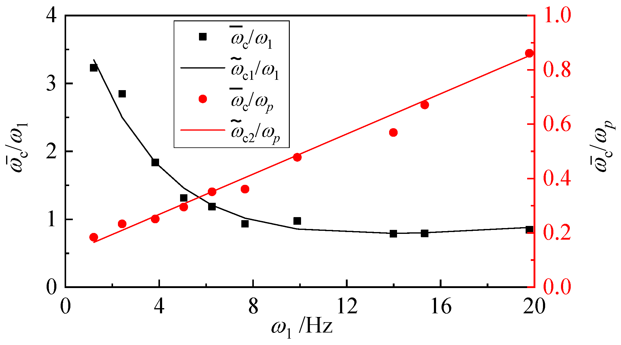
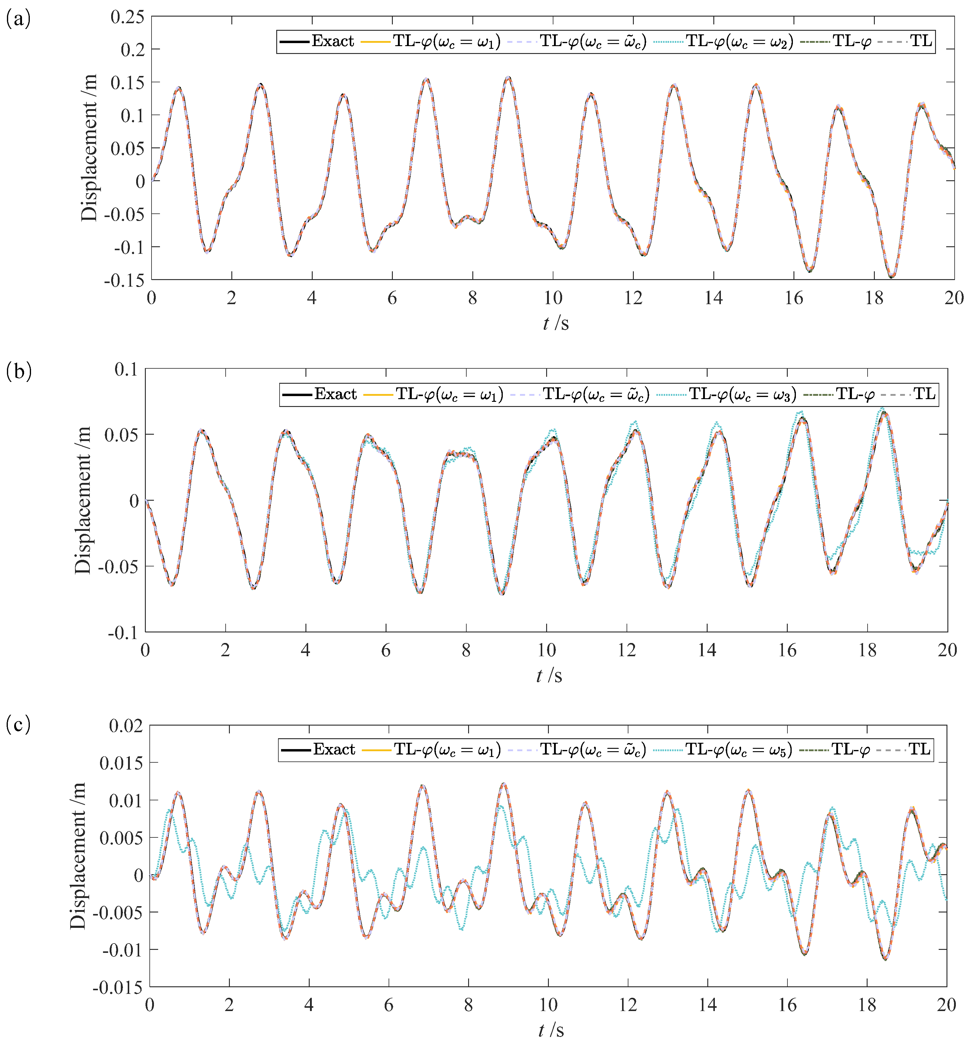
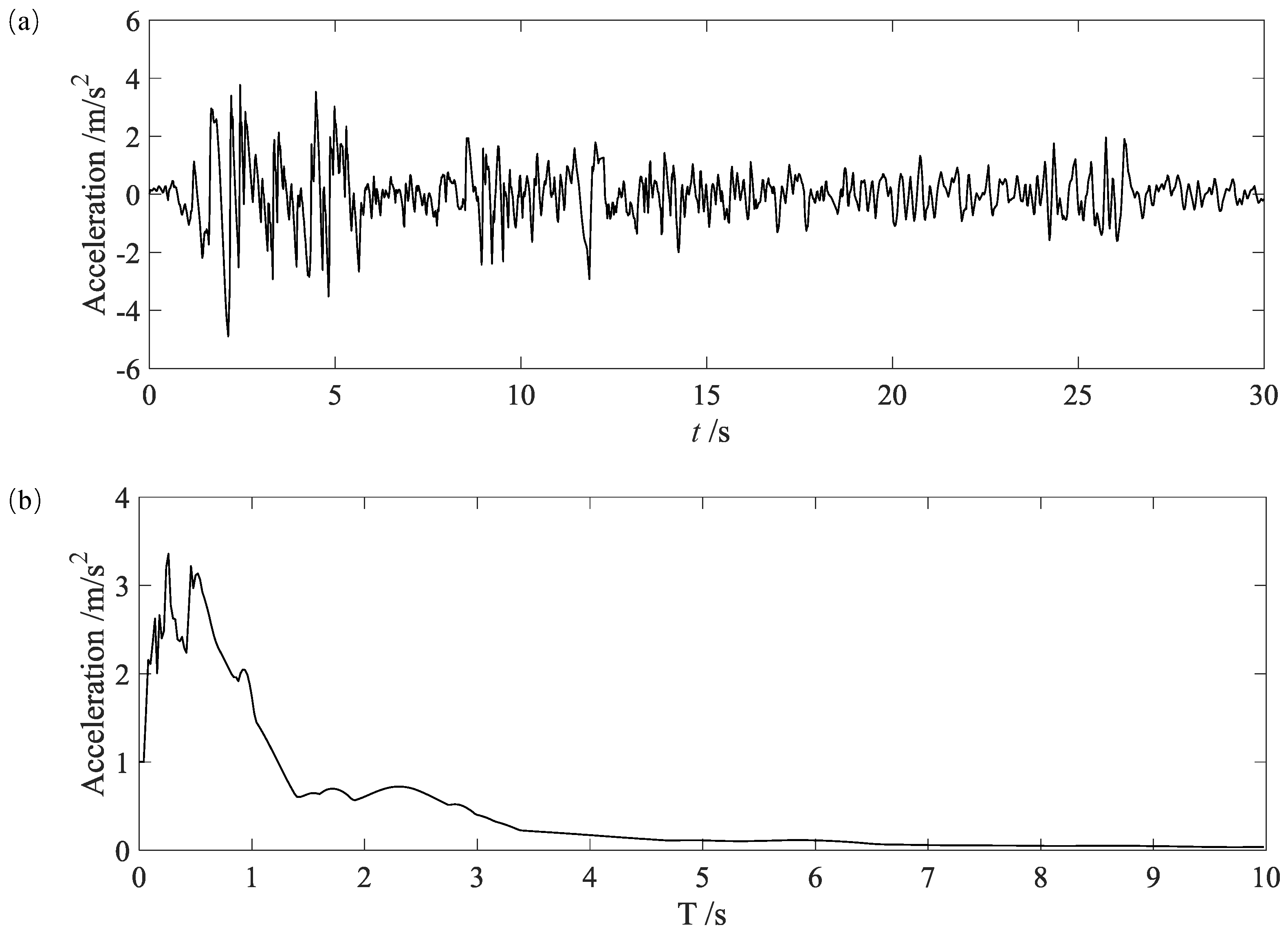
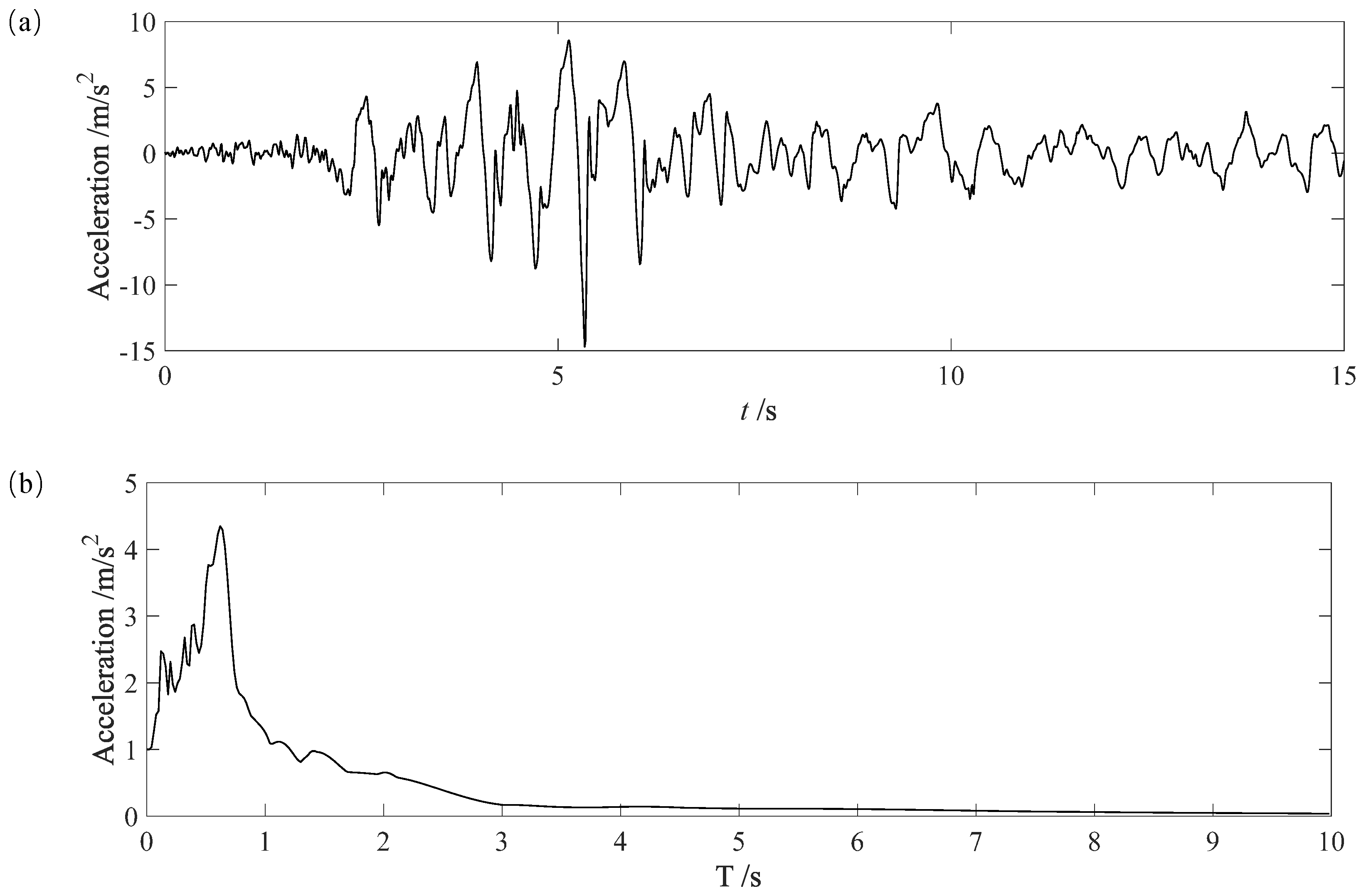
Numerical analysis of the 20-DOF spring-mass system is performed to establish a selection criterion of ${\omega }_c$. A total of 14 seismic waves are selected as external excitations, and ${\omega }_p$ of each wave is shown in

Table 3. Peak frequency of response spectrum (rad/s).

Earthquake	${\mathit{\omega }}_{\mathit{p}}$	Earthquake	${\mathit{\omega }}_{\mathit{p}}$	Earthquake	${\mathit{\omega }}_{\mathit{p}}$
El Centro	24.166	San Fernando1	19.635	Chuetsu-oki	20.944
Taft	14.280	San Fernando2	17.453	Victoria Mexico	44.880
Wen Chuan	52.359	San Fernando3	14.960	Loma Prieta	10.134
Irpinia Italy	34.906	Corinth Greece	12.083	San Simeon	28.560
Tottori Japan	31.416	Cape Mendocino	18.580	Artificial Wave	15.708

. Moreover, 10 groups of structural properties are designed to investigate the relationship between ${\omega }_c$ and ${\omega }_p$ as well as ${\omega }_1$.

TL-$\phi$ algorithms with ${\omega }_c$ varying from 1 rad/s to 20 rad/s are applied to calculate NRMSE for each model. It is worth noting that the minimal NRMSE can be obtained when ${\omega }_c={\omega }_1$ for the case of ${\omega }_p\le {\omega }_1$. For ${\omega }_p>{\omega }_1$, the optimal critical frequencies ${\widehat{\omega }}_c$ and the arithmetic mean values ${\overline{\omega }}_c$ are acquired according to Equation (15).

Table 4. Ratios of the average values of ${\overline{\omega }}_c$ to ${\omega }_1$ and ${\omega }_p$.

Model	1	2	3	4	5
${\omega }_1$$/\mathrm{rad}/\mathrm{s}$	1.2112	2.4225	3.8303	5.0512	6.2548
${\overline{\omega }}_{c1}/{\omega }_1$	3.228	2.847	1.836	1.314	1.186
${\overline{\omega }}_{c2}/{\omega }_p$	0.184	0.350	0.342	0.295	0.351
Model	6	7	8	9	10
${\omega }_1$$/\mathrm{rad}/\mathrm{s}$	7.6605	9.8897	11.4197	13.9862	15.3211
${\overline{\omega }}_{c1}/{\omega }_1$	0.934	0.974	0.895	0.785	0.848
${\overline{\omega }}_{c2}/{\omega }_p$	0.361	0.478	0.496	0.569	0.671

lists the ratio of the mean values of ${\overline{\omega }}_c$ to ${\omega }_1$ and ${\omega }_p$ for each model. Figure 5 shows the scatter diagram of mean values varying with ${\omega }_1$, which indicates that ${\overline{\omega }}_c/{\omega }_1$ decays exponentially with an increasing of ${\omega }_1$, while ${\overline{\omega }}_c/{\omega }_p$ increases linearly with an increasing of ${\omega }_1$. The fitting formulas are also conducted based on the regression analysis as follows, and the ${\omega }_c$ that equals to the smaller one of ${\tilde{\omega }}_{c1}$ and ${\tilde{\omega }}_{c2}$ is recommended in this situation.

$$\frac{{\tilde{\omega }}_{c1}}{{\omega }_1}=4.2e^{-0.3{\omega }_1}+0.4e^{0.05{\omega }_1},1.2\le {\omega }_1\le 20$$

(20)

$$\frac{{\tilde{\omega }}_{c2}}{{\omega }_p}=0.037{\omega }_1+0.12,1.2\le {\omega }_1\le 20$$

(21)

$${\tilde{\omega }}_c=\mathbf{min}({\tilde{\omega }}_{c1},{\tilde{\omega }}_{c2})$$

(22)

$$\begin{array}{c}\hfill \begin{array}{c}\hfill {\omega }_c=\left\{\begin{array}{cc}{\omega }_1,\hfill & {\omega }_p\le {\omega }_1\hfill \\ {\tilde{\omega }}_c,\hfill & {\omega }_p>{\omega }_1\hfill \end{array}\right.\end{array}\end{array}$$

(23)

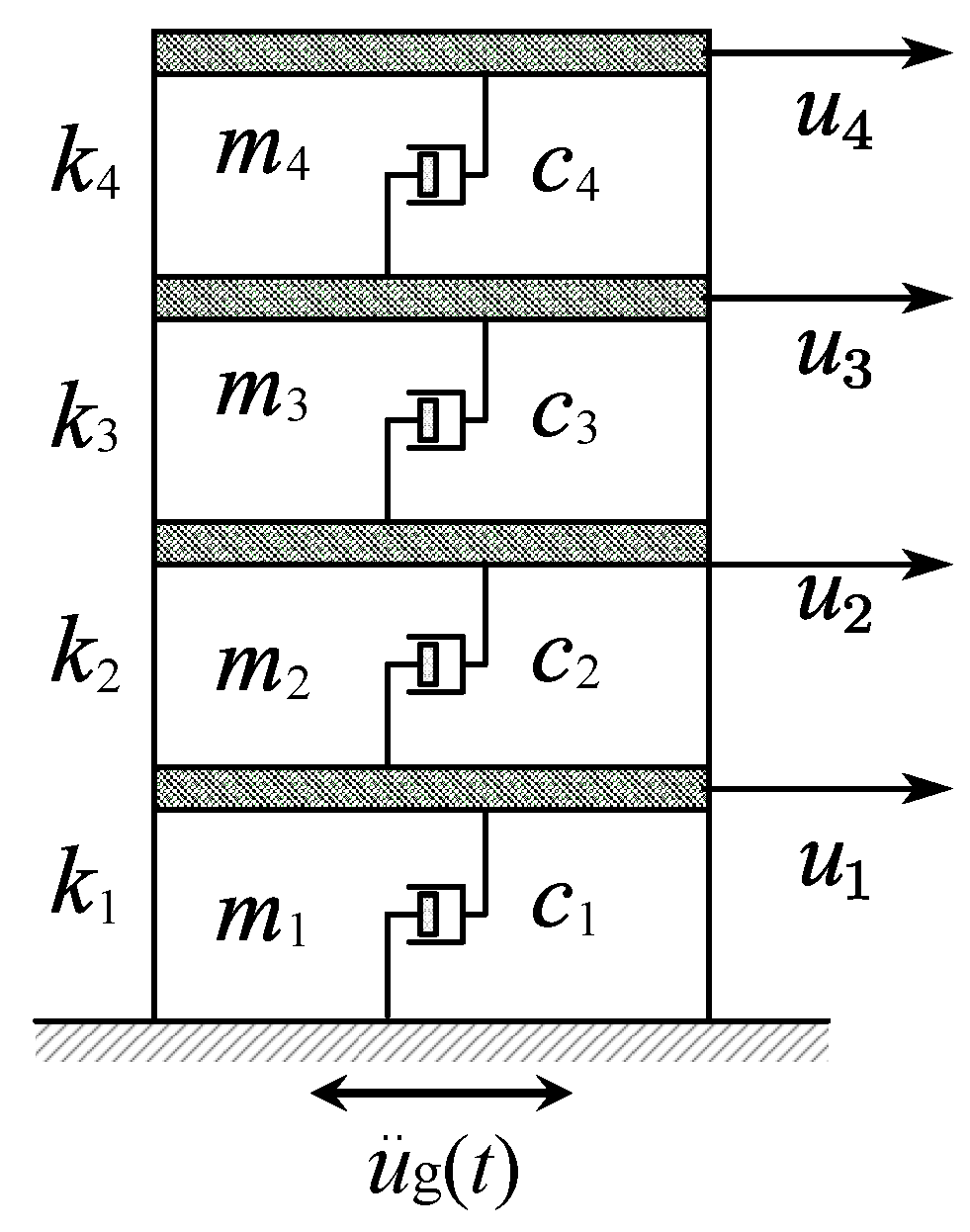
4.2. Modal Participation Factor, MPF

Another factor that rules the importance of any mode in the total dynamic response is MPF. In Equation (6), the external force vector $\mathbf{F}\left(t\right)$ can be expressed as a product of a distribution vector $\mathbf{R}$ and an amplitude vector $p\left(t\right)$:

$$\mathbf{F}\left(t\right)=\mathbf{R}p\left(t\right)$$

(24)

and for the particular case of seismic excitation, it has

$$\mathbf{F}\left(t\right)=\mathbf{Mr}{\ddot{u}}_g\left(t\right)$$

(25)

where, $\mathbf{r}$ is a displacement transformation vector that expresses the displacement of each DOF excited by a unit static support displacement.

Introducing Equation (24) or (25) into Equation (6), the equation of motion for each DOF becomes:

$${\ddot{y}}_n\left(t\right)+2{\xi }_n{\omega }_n{\dot{y}}_n\left(t\right)+{\omega }_n^2{y}_n\left(t\right)=\frac{{\mathit{\varphi }}_n^{\mathrm{T}}\mathbf{R}}{{\mathit{\varphi }}_n^{\mathrm{T}}\mathbf{M}{\mathit{\varphi }}_n}p\left(t\right)$$

(26)

or

$${\ddot{y}}_n\left(t\right)+2{\xi }_n{\omega }_n{\dot{y}}_n\left(t\right)+{\omega }_n^2{y}_n\left(t\right)=\frac{{\mathit{\varphi }}_n^{\mathrm{T}}\mathbf{Mr}}{{\mathit{\varphi }}_n^{\mathrm{T}}\mathbf{M}{\mathit{\varphi }}_n}{\ddot{u}}_g\left(t\right)$$

(27)

The ratios shown on the right side of Equations (26) and (27) are defined as the modal participation factor. That is,

$${\mathrm{MPF}}_n=\frac{{\mathit{\varphi }}_n^{\mathrm{T}}\mathbf{R}}{{\mathit{\varphi }}_n^{\mathrm{T}}\mathbf{M}{\mathit{\varphi }}_n}\mathrm{or}{\mathrm{MPF}}_n=\frac{{\mathit{\varphi }}_n^{\mathrm{T}}\mathbf{Mr}}{{\mathit{\varphi }}_n^{\mathrm{T}}\mathbf{M}{\mathit{\varphi }}_n}$$

(28)

It is apparent from Equation (28) that the amplitude of the response due to any given mode depends on the interaction of the applied load distribution and the mode shape. An arbitrary external load distribution applied to an engineering structure might excite a response in any of the modes, and it is recommended that ${\omega }_c$ equals to the frequency corresponding to the mode with the largest value of MPF. While for an engineering structure subjected to horizontal ground motion, the transformation vector $\mathbf{r}$ is a unit column, and the determination of ${\omega }_c$ depends mainly on DMF.

5. Numerical Confirmations

For numerical confirmation of the selection criterion for ${\omega }_c$ proposed in this paper, three cases with different original structural properties and loading conditions are intentionally designed.

5.1. Case 1: Undamped Linear MDOF System under Harmonic Ground Motion

A spring-mass system with 50-DOF is utilized to discuss the effect of ${\omega }_c$ selected for $\phi$ on dynamic responses, and its structural properties are plotted in Figure 6. After the eigenvalue-analysis, the lowest natural frequency of the system is found to be 3.1104 rad/s, while the highest natural frequency is found to be 199.90 rad/s.

Table 5. The first 10 natural frequencies and MPFs of the system.

Mode	Frequency (rad/s)	MPF (%)	Mode	Frequency (rad/s)	MPF (%)
1	3.1104	36.804	6	34.049	3.3133
2	9.3281	12.260	7	40.161	2.7926
3	15.537	7.3465	8	46.235	2.4091
4	21.730	5.2373	9	52.264	2.1144
5	27.903	4.0629	10	58.243	1.8805

shows the first 10 natural frequencies and the corresponding MPFs of the system. The system is subjected to a harmonic acceleration excitation of sine-wave form at the ground, and the circular frequency $\tilde{\omega }$ is set to 1, 6, 16 and 40 rad/s, respectively.

According to the selection criterion of ${\omega }_c$ in Equation (19), ${\omega }_c={\omega }_1$ when $\tilde{\omega }=$ 1 and 6 rad/s; ${\omega }_c={\omega }_3$ when $\tilde{\omega }=16$ rad/s; ${\omega }_c={\omega }_7$ when $\tilde{\omega }=40$ rad/s, and the corresponding $\phi =0.9999,0.9980,0.9869$, respectively. Numerical results obtained from TL-$\phi$ algorithm with different values of ${\omega }_c$ and other three well-developed algorithms, including Chang algorithm, CR algorithm and TL algorithm, with $\Delta t=0.01$ s are shown in Figure 7a–d. In the figures, the analytical solutions obtained by modal superposition method (MSM) are marked as “Exact” for comparison, and “TL-$\mathit{\phi }$” refers to the ones derived from TL-$\phi$ algorithm with precorrecting for each mode. It is worth noting that the displacements obtained from TL-$\phi$ algorithm are nearly in total agreement with the exact solution for all the loading conditions while those obtained from the other three algorithms possess obvious period distortions and amplitude errors.

Table 6. Displacement errors for $m_{50}$ ($\tilde{\omega }=1\mathrm{rad}/\mathrm{s}$, %).

Error Index	TL-$\mathit{\phi }({\mathit{\omega }}_{\mathit{c}}={\mathit{\omega }}_1)$	TL-$\mathit{\phi }({\mathit{\omega }}_{\mathit{c}}={\mathit{\omega }}_{\mathit{p}})$	TL-$\mathit{\phi }$	Chang/CR/TL
NEE	0.0057	0.0072	0.0048	0.0074
NRMSE	0.0091	0.0249	0.0014	0.0273

,

Table 7. Displacement errors for $m_{50}$ ($\tilde{\omega }=6\mathrm{rad}/\mathrm{s}$, %).

Error Index	TL-$\mathit{\phi }({\mathit{\omega }}_{\mathit{c}}={\mathit{\omega }}_1)$	TL-$\mathit{\phi }({\mathit{\omega }}_{\mathit{c}}={\mathit{\omega }}_{\mathit{p}})$	TL-$\mathit{\phi }$	Chang/CR/TL
NEE	0.0120	0.0805	0.0046	0.0461
NRMSE	0.1062	0.1978	0.0057	0.1329

,

Table 8. Displacement errors for $m_{50}$ ($\tilde{\omega }=16\mathrm{rad}/\mathrm{s}$, %).

Error Index	TL-$\mathit{\phi }({\mathit{\omega }}_{\mathit{c}}={\mathit{\omega }}_1)$	TL-$\mathit{\phi }({\mathit{\omega }}_{\mathit{c}}={\mathit{\omega }}_3)$	TL-$\mathit{\phi }({\mathit{\omega }}_{\mathit{c}}={\mathit{\omega }}_{\mathit{p}})$	TL-$\mathit{\phi }$	Chang/CR/TL
NEE	2.7093	0.2905	0.4701	0.00001	2.8479
NRMSE	3.1614	1.0127	1.0930	0.0414	3.2922

and

Table 9. Displacement errors for $m_{50}$ ($\tilde{\omega }=40\mathrm{rad}/\mathrm{s}$, %).

Error Index	TL-$\mathit{\phi }({\mathit{\omega }}_{\mathit{c}}={\mathit{\omega }}_1)$	TL-$\mathit{\phi }({\mathit{\omega }}_{\mathit{c}}={\mathit{\omega }}_7)$	TL-$\mathit{\phi }({\mathit{\omega }}_{\mathit{c}}={\mathit{\omega }}_{\mathit{p}})$	TL-$\mathit{\phi }$	Chang/CR/TL
NEE	63.224	5.4002	6.6519	4.6284	63.793
NRMSE	24.353	7.0159	7.0351	1.6679	24.356

list two error indicators, including the aforementioned NRMSE and normalized energy error (NEE), for displacement responses of the system ($m_{50}$) under harmonic excitation with different $\tilde{\omega }$. In general, NEE reflects signal energy and is sensitive to amplitude differences of the dynamic responses, defined as

$$\mathrm{NEE}=\left|\frac{{\sum }_{i=1}^m{u}_{\mathrm{ES},i}^2-{\sum }_{i=1}^m{u}_{\mathrm{NS},i}^2}{{\sum }_{i=1}^m{u}_{\mathrm{NS},i}^2}\right|$$

(29)

where, the meaning of the subscript NS, ES and m are the same as those for NRMSE in Equation (14).

It is worth noting that both NEE and NRMSE are the minimum for “TL-$\mathit{\phi }$” in any case, confirming that precorrecting for each mode of an MDOF system will achieve great accuracy. In addition, the value of ${\omega }_c$ chosen for $\phi$ has a noticeable effect on the two errors, especially when the system suffers from a rather high excitation frequency. An appropriate value of ${\omega }_c$ chosen for $\phi$ will result in relatively smaller errors in both amplitude and period when compared with other algorithms. This verifies the effectiveness of the proposed criterion in selecting ${\omega }_c$ when applying the TL-$\phi$ algorithm to MDOF systems.

5.2. Case 2: Undamped Linear MDOF System under Arbitrary Load

A five-story shear building under an arbitrary load is shown in Figure 8. Two groups of the structural property are intentionally designed to investigate the effect of MPF on determining ${\omega }_c$, including (1) $m_i={10}^5$ kg, $k_i={10}^7$ N/m ($i=1,2\dots 5$); (2) $m_1={10}^7$ kg, $m_2=m_3={10}^5$ kg, $m_4=m_5={10}^3$ kg, and $k_i={10}^7$ N/m ($i=1,2\dots 5$). The initial natural frequencies and the modal shapes of the building for the two groups (labelled G1 and G2) are shown in

Table 10. Natural frequencies and modal shapes of the building (G1).

Mode	Frequency/rad/s	$\mathsf{\Phi }$
		${\mathbf{\varphi }}_{\mathbf{1}}$	${\mathbf{\varphi }}_{\mathbf{2}}$	${\mathbf{\varphi }}_{\mathbf{3}}$	${\mathbf{\varphi }}_{\mathbf{4}}$	${\mathbf{\varphi }}_{\mathbf{5}}$
1	2.8463	0.2846	0.7635	1.0000	0.9190	0.5462
2	8.3083	0.5462	1.0000	0.2846	−0.7636	−0.9190
3	13.097	0.7635	0.5462	−0.9190	−0.2846	1.0000
4	16.825	0.9190	−0.2846	−0.5462	1.0000	−0.7635
5	19.190	1.0000	−0.9190	0.7635	−0.5462	0.2846

and

Table 11. Natural frequencies and modal shapes of the building (G2).

Mode	Frequency/rad/s	$\mathsf{\Phi }$
		${\mathbf{\varphi }}_{\mathbf{1}}$	${\mathbf{\varphi }}_{\mathbf{2}}$	${\mathbf{\varphi }}_{\mathbf{3}}$	${\mathbf{\varphi }}_{\mathbf{4}}$	${\mathbf{\varphi }}_{\mathbf{5}}$
1	0.9898	0.9700	−0.0165	−0.0039	0.0000	0.0000
2	6.1955	0.9897	0.6014	1.0000	0.0000	0.0000
3	16.142	0.9997	0.9885	−0.6019	−0.0165	−0.0038
4	62.401	0.9999	0.9962	−0.6354	0.6106	1.0000
5	161.89	1.0000	1.0000	−0.6524	1.0000	−0.6170

.

The building is excited by an arbitrary load $\mathbf{F}={[f_1,f_2,f_3,f_4,f_5]}^T$ with a spatial load distribution vector of $\mathbf{R}$, i.e., $\mathbf{F}\left(t\right)=\mathbf{R}·p_0\sin \left(\tilde{\omega }t\right)$. In this case, $p_0=100$ kN and $\tilde{\omega }=3$ rad/s are employed. Considering $\mathbf{R}={\varphi }_2$, ${\varphi }_3$ and ${\varphi }_5$, this will accentuate the responses in the 2nd, 3rd and 5th mode of the building, respectively. The corresponding ${\omega }_c$ selected in this case should be equal to ${\omega }_2$, ${\omega }_3$ and ${\omega }_5$ based on the proposed criterion of MPF, and then $\phi =0.9977,0.9943,0.9880$ for G1 while $\phi =0.9987,0.9914,0.6285$ for G2, respectively. The displacement responses obtained from the Newmark algorithm with [$\alpha ,\beta$] = [1/2, 1/4] and $\Delta t=0.005$ s are considered as the “Exact” solution for comparison, while the time step of $\Delta t=0.02$ s is employed to compute the seismic responses for using TL-$\phi$ algorithms and TL algorithm. Numerical results for the initial conditions of $\mathbf{U}=\mathbf{0}$ m, $\dot{\mathbf{U}}=\mathbf{0}$ m/s are displayed in the following. Figure 9 shows the displacement responses of the 5th story for G1 while those for G2 are plotted in Figure 10. Errors of the displacement responses for G1 and G2 are listed in

Table 12. Displacement errors of the 5th floor (G1).

R	Error Index	TL-$\mathit{\phi }\mathbf{(}{\mathit{\omega }}_{\mathit{c}}\mathbf{=}{\mathit{\omega }}_{\mathbf{1}}\mathbf{)}$	TL-$\mathit{\phi }\mathbf{(}{\mathit{\omega }}_{\mathit{c}}\mathbf{=}{\mathit{\omega }}_2\mathbf{)}$	TL-$\mathit{\phi }$	TL
${\varphi }_2$	NEE	0.3915	0.1559	0.1559	0.4186
	NRMSE	1.4177	0.6355	0.6355	1.6489
R	Error Index	TL-$\mathit{\phi }\mathbf{(}{\mathit{\omega }}_{\mathit{c}}\mathbf{=}{\mathit{\omega }}_{\mathbf{1}}\mathbf{)}$	TL-$\mathit{\phi }\mathbf{(}{\mathit{\omega }}_{\mathit{c}}\mathbf{=}{\mathit{\omega }}_{\mathbf{3}}\mathbf{)}$	TL-$\mathit{\phi }$	TL
${\varphi }_3$	NEE	0.5104	0.1625	0.1625	0.5247
	NRMSE	4.5327	0.8258	0.8258	4.7661
R	Error Index	TL-$\mathit{\phi }\mathbf{(}{\mathit{\omega }}_{\mathit{c}}\mathbf{=}{\mathit{\omega }}_{\mathbf{1}}\mathbf{)}$	TL-$\mathit{\phi }\mathbf{(}{\mathit{\omega }}_{\mathit{c}}\mathbf{=}{\mathit{\omega }}_{\mathbf{5}}\mathbf{)}$	TL-$\mathit{\phi }$	TL
${\varphi }_5$	NEE	0.4686	0.1969	0.1969	0.4709
	NRMSE	7.4568	1.0506	1.0506	7.4800

and

Table 13. Displacement errors of the 5th floor (G2).

R	Error Index	TL-$\mathit{\phi }\mathbf{(}{\mathit{\omega }}_{\mathit{c}}\mathbf{=}{\mathit{\omega }}_{\mathbf{1}}\mathbf{)}$	TL-$\mathit{\phi }\mathbf{(}{\mathit{\omega }}_{\mathit{c}}\mathbf{=}{\tilde{\mathit{\omega }}}_{\mathit{c}}\mathbf{)}$	TL-$\mathit{\phi }\mathbf{(}{\mathit{\omega }}_{\mathit{c}}\mathbf{=}{\mathit{\omega }}_{\mathbf{2}}\mathbf{)}$	TL-$\mathit{\phi }$	TL
${\varphi }_2$	NEE	0.3415	0.3382	0.1407	0.1163	0.3470
	NRMSE	0.8922	0.8842	0.7590	0.7358	0.9059
R	Error Index	TL-$\mathit{\phi }\mathbf{(}{\mathit{\omega }}_{\mathit{c}}\mathbf{=}{\mathit{\omega }}_{\mathbf{1}}\mathbf{)}$	TL-$\mathit{\phi }\mathbf{(}{\mathit{\omega }}_{\mathit{c}}\mathbf{=}{\tilde{\mathit{\omega }}}_{\mathit{c}}\mathbf{)}$	TL-$\mathit{\phi }\mathbf{(}{\mathit{\omega }}_{\mathit{c}}\mathbf{=}{\mathit{\omega }}_{\mathbf{3}}\mathbf{)}$	TL-$\mathit{\phi }$	TL
${\varphi }_3$	NEE	0.3230	0.3202	0.6018	0.1138	0.3276
	NRMSE	1.1331	1.1281	4.1863	0.9102	1.1418
R	Error Index	TL-$\mathit{\phi }\mathbf{(}{\mathit{\omega }}_{\mathit{c}}\mathbf{=}{\mathit{\omega }}_{\mathbf{1}}\mathbf{)}$	TL-$\mathit{\phi }\mathbf{(}{\mathit{\omega }}_{\mathit{c}}\mathbf{=}{\tilde{\mathit{\omega }}}_{\mathit{c}}\mathbf{)}$	TL-$\mathit{\phi }\mathbf{(}{\mathit{\omega }}_{\mathit{c}}\mathbf{=}{\mathit{\omega }}_{\mathbf{5}}\mathbf{)}$	TL-$\mathit{\phi }$	TL
${\mathit{\varphi }}_{\mathbf{5}}$	NEE	0.4934	0.3865	109.34	0.2195	0.5015
	NRMSE	1.0423	0.7724	27.200	0.8470	1.0666

.

Regarding G1, it can be seen from Figure 9a–c that the displacements derived from the TL-$\phi$ algorithm with ${\omega }_c={\omega }_2$ for $\mathbf{R}={\varphi }_2$, ${\omega }_c={\omega }_3$ for $\mathbf{R}={\varphi }_3$ and ${\omega }_c={\omega }_5$ for $\mathbf{R}={\varphi }_5$ are almost in total agreement with the “Exact” solution. Displacement errors shown in Table 12 distinctly indicate that a much higher accuracy can be obtained when ${\omega }_c$ is equal to the frequency corresponding to the mode with the largest value of MPF. For G2, it can be seen in Figure 10a–c and Table 13 that TL-$\phi$ algorithm with ${\omega }_c={\tilde{\omega }}_c$ can result in a better solution while larger errors are found in the results obtained from TL-$\phi$ algorithm with ${\omega }_c={\omega }_i(i=2,3,5)$. This illustrates that the availability of determining ${\omega }_c$ based on MPF depends on the mass distribution of the system. The more evenly the mass is distributed, the greater the influence of MPF on determining ${\omega }_c$. On the contrary, the determination of ${\omega }_c$ should depend mainly on DMF.

5.3. Case 3: Damped Linear MDOF System under Seismic Input

A four-story shear building under seismic input is shown in Figure 11. The structural properties are $m_1={10}^5$ kg, $m_2=m_3={10}^4$ kg, $m_4={10}^3$ kg, $k_i={10}^7$ N/m ($i=1,2,3,4$), and the natural frequencies are 8.88, 21.08, 50.65, and 105.41 rad/s. Assuming Rayleigh Damping, the damping matrix can be determined by combining the mass and the stiffness matrices as follows,

$$\mathbf{C}=a_0\mathbf{M}+a_1\mathbf{K}$$

(30)

in which, $a_0$ and $a_1$ are the two proportionality factors evaluated by the following equation:

$$\left\{\begin{array}{c}{a}_0\hfill \\ a_1\hfill \end{array}\right\}=\frac{2\xi }{{\omega }_1+{\omega }_3}\left\{\begin{array}{c}{\omega }_1{\omega }_3\\ 1\end{array}\right\}$$

(31)

where, $\xi =0.05$ is the damping ratio; ${\omega }_1$ and ${\omega }_3$ are the two specific frequencies selected for Rayleigh Damping.

The system is subjected to the ground acceleration record of the El Centro wave, where the peak ground acceleration (PGA) is scaled to 0.5 g. The sampling interval of the record is 0.02 s. The time history and response spectrum of the El Centro wave are shown in Figure 12, noting that the peak frequency of the response spectrum ${\omega }_p=24.166$ rad/s.

Numerical results for the initial conditions of $u\left(0\right)=0$ m and $\dot{u}\left(t\right)=0$ m/s are displayed in Figure 13, where the numerical solution obtained from the Newmark algorithm with [$\alpha ,\beta$] = [1/2, 1/4] and $\Delta t=0.005$ s is considered as a reference solution for comparison. TL-$\phi$ algorithms with the time step of 0.02 s are applied to perform the step-by-step integration. Based on the proposed selection criterion in Equations (20)–(22), ${\omega }_c=\mathbf{min}({\tilde{\omega }}_{c1},{\tilde{\omega }}_{c2})=8.14$ rad/s and $\phi =0.9978$. Displacement errors of the 4th story derived from TL-$\phi$ algorithms with different values of ${\omega }_c$ are shown in

Table 14. Displacement errors for the 4th story.

Error Index	TL-$\mathit{\phi }({\mathit{\omega }}_{\mathit{c}}=8.14$ rad/s)	TL-$\mathit{\phi }({\mathit{\omega }}_{\mathit{c}}={\mathit{\omega }}_1)$	TL-$\mathit{\phi }({\mathit{\omega }}_{\mathit{c}}={\mathit{\omega }}_{\mathit{p}})$	TL-$\mathit{\phi }$
NEE	0.7147	1.1606	16.039	1.7891
NRMSE	0.5929	0.6582	4.1664	0.6330

. It can be seen that both NEE and NRMSE are minimal for “TL-$\phi ({\omega }_c=8.14$ rad/s)”, indicating that the proposed selection criterion of ${\omega }_c$ is applicable for an MDOF that is subjected to a seismic wave.

5.4. Case 4: An MDOF System with Softening Stiffness

The five-story shear building shown in Figure 8 is used in this case. The initial structural properties are $m_i={10}^5$ kg, $k_{i,0}={10}^7$ N/m ($i=1,2\dots 5$), $\xi =0.02$, and the natural frequencies are as shown in Table 10. The softening stiffness of the system after deformation is designated as $k_i=k_{i,0}(1-\sqrt{\left|u_i-u_{i-1}\right|})$, where subscript i refers to the ith story and $(u_i-u_{i-1})$ is the inter-story drift of the ith story.

The system with zero initial conditions is subjected to the ground acceleration record of the Loma Prieta wave, where PGA = 1.05 g. The sampling interval of the record is 0.01 s. The time history and response spectrum of the Loma Prieta wave are shown in Figure 14, noting that the peak frequency of the response spectrum ${\omega }_p=10.134$ rad/s.

TL-$\phi$ algorithms with the time step of 0.01 s are applied to perform the step-by-step integration, while the numerical solution obtained from the Newmark algorithm with [$\alpha ,\beta$] = [1/2, 1/4] and $\Delta t=0.005$ s is considered as a reference solution for comparisons. According to the proposed selection criterion in Equations (20)–(22), ${\omega }_c=\mathbf{min}({\tilde{\omega }}_{c1},{\tilde{\omega }}_{c2})=2.28$ rad/s and $\phi \approx 1.0000$. Displacement errors of the 4th story derived from TL-$\phi$ algorithms with different values of ${\omega }_c$ are shown in

Table 15. Displacement errors for the 4th story.

Error Index	TL-$\mathit{\phi }({\mathit{\omega }}_{\mathit{c}}=2.28$ rad/s)	TL-$\mathit{\phi }({\mathit{\omega }}_{\mathit{c}}={\mathit{\omega }}_1)$	TL-$\mathit{\phi }({\mathit{\omega }}_{\mathit{c}}={\mathit{\omega }}_{\mathit{p}})$	TL-$\mathit{\phi }$
NEE	4.9178	4.9193	4.9808	5.0293
NRMSE	0.8277	0.8312	0.9501	0.8514

, and the responses are ploted in Figure 15. It can be seen that both NEE and NRMSE are minimal for “TL-$\phi ({\omega }_c=2.28$ rad/s)”, indicating that the proposed selection criterion of ${\omega }_c$ is still applicable for non-linear MDOF systems.

6. Conclusions

TL-$\phi$ algorithms represent newly proposed SDIM that possess controllable numerical dispersion properties by introducing a precorrection parameter $\phi$. This precorrection parameter depends on the critical frequency ${\omega }_c$ of a system. When TL-$\phi$ algorithms are applied to an MDOF system, the first and most important issue is the determination of ${\omega }_c$ for $\mathit{\phi }$. Precorrection for each frequency (mode) of the system may achieve high accuracy, but is time consuming especially when the number of DOFs is huge. Indeed, relatively high accuracy of the dynamic responses can still be obtained by precorrecting a specific mode (deemed to be ${\omega }_c$) that dominates the total responses of an MDOF system, and then $\mathit{\phi }$ will reduce to a constant scaling $\phi$ for all the modes of the system.

In this work, the choices of ${\omega }_c$ are fully discussed by investigating the relationship between ${\omega }_c$ and ${\omega }_1$ as well as $\tilde{\omega }$ (or ${\omega }_p$). It is worth noting that the value of ${\omega }_c$ selected for $\phi$ has a significant influence on the structural responses, and its determination should consider both the initial structural properties of the system and the numerical characteristics of external excitation. Two factors that control the importance of any mode in the total dynamic responses, including DMF and MPF, are taken into account to obtain the optimal critical frequency. Empirical formulas of ${\omega }_c$ for systems subjected to both harmonic excitation and seismic waves are obtained by numerical calculation of NRMSE. A total of four numerical cases are intentionally designed to examine the feasibility of the selection criterion ${\omega }_c$ proposed in this work. By studying the two error indicators of NEE and NRMSE, it is illustrated that a smaller period distortion in dynamic responses derived from TL-$\phi$ algorithms can be achieved when ${\omega }_c$ is determined according to the proposed criterion. This will lead to further improvements of the numerical dispersion property of TL-$\phi$ algorithms in solving structural dynamic problems of MDOF systems.

References

1. Darby, A.; Blakeborough, A.; Williams, M. Improved control algorithm for real-time substructure testing. Earthq. Eng. Struct. Dyn. 2001, 30, 431–448. [Google Scholar] [CrossRef]
2. Bonnetr, P.; Williams, M.; Blakeboroughg, A. Evaluation of numerical time-integration schemes for real-time hybrid testing. Earthq. Eng. Struct. Dyn. 2008, 37, 1467–1490. [Google Scholar] [CrossRef]
3. Chang, S. Choices of structure-dependent pseudodynamic algorithms. J. Eng. Mech. 2019, 145, 04019029. [Google Scholar] [CrossRef]
4. Newmark, N. A method of computation for structural dynamics. J. Eng. Mech. 1959, 85, 67–94. [Google Scholar] [CrossRef]
5. Wilson, E.; Farhoomand, I.; Bathe, K. Nonlinear dynamic analysis of complex structure. Earthq. Eng. Struct. Dyn. 1973, 1, 241–252. [Google Scholar] [CrossRef]
6. Hilber, H.; Hughes, T.; Taylor, R. Improved numerical dissipation for time integration algorithms in structural mechanics. Earthq. Eng. Struct. Dyn. 1977, 5, 283–292. [Google Scholar] [CrossRef] [Green Version]
7. Butcher, J. A history of Runge–Kutta methods. Appl. Numer. Math. 1996, 20, 247–260. [Google Scholar] [CrossRef]
8. Bhrawy, A. An efficient Jacobi pseudospectral approximation for nonlinear complex generalized Zakharov system. Appl. Math. Comput. 2014, 247, 30–46. [Google Scholar] [CrossRef]
9. Momeni, M.; Riahi Beni, M.; Bedon, C.; Najafgholipour, M.; Dehghan, S.; JavidSharifi, B.; Hadianfard, M. Dynamic Response Analysis of Structures Using Legendre–Galerkin Matrix Method. Appl. Sci. 2021, 11, 9307. [Google Scholar] [CrossRef]
10. Ertürk, V.; Momani, S. Solving systems of fractional differential equations using differential transform method. J. Comput. Appl. Math. 2008, 215, 142–151. [Google Scholar] [CrossRef] [Green Version]
11. Pakdemirli, M.; Karahan, M.M.F.; Boyacı, H. Forced Vibrations of Strongly Nonlinear Systems with Multiple Scales Lindstedt Poincaré Method. Math. Comput. Appl. 2011, 16, 879–889. [Google Scholar] [CrossRef] [Green Version]
12. Rysak, A.; Magdalena, G. Differential Transform Method as an Effective Tool for Investigating Fractional Dynamical Systems. Appl. Sci. 2021, 11, 6955. [Google Scholar] [CrossRef]
13. Mahin, S.; Shing, P. Pseudodynamic method for seismic testing. J. Eng. Mech. 1985, 111, 1482–1509. [Google Scholar] [CrossRef]
14. Tang, Y.; Qin, H. Stability and Accuracy Analysis of Real-Time Hybrid Simulation (RTHS) with Incomplete Boundary Conditions and Actuator Delay. Int. J. Struct. Stab. Dyn. 2020, 20, 2050122. [Google Scholar] [CrossRef]
15. Chang, S.; Wu, T.; Tran, N.; Yang, Y. Apllications of a Family of Unconditionally stable, Dissipative, Explicit methods to pseudodynamic tests. Exp. Tech. 2017, 41, 19–36. [Google Scholar] [CrossRef]
16. Chang, S. Explicit pseudodynamic algorithm with unconditional stability. J. Eng. Mech. 2002, 128, 935–947. [Google Scholar] [CrossRef]
17. Chen, C.; Ricles, J. Development of direct integration algorithms for structural dynamics using discrete control theory. J. Eng. Mech. 2008, 134, 676–683. [Google Scholar] [CrossRef]
18. Rezaiee-Pajand, M.; Hashemian, M. Time Integration Method Based on Discrete Transfer Function. Int. J. Struct. Stab. Dyn. 2016, 16, 1550009. [Google Scholar] [CrossRef]
19. Tang, Y.; Lou, M. New unconditionally stable explicit integration algorithm for real-time hybrid testing. J. Eng. Mech. 2017, 143, 04017029. [Google Scholar] [CrossRef]
20. Tang, Y.; Qin, H. Applications of the RST Algorithm to Nonlinear Systems in Real-Time Hybrid Simulation. Math. Probl. Eng. 2020, 2020, 5734720. [Google Scholar] [CrossRef]
21. Chang, S. Improved explicit method for structural dynamics. J. Eng. Mech. 2007, 133, 748–760. [Google Scholar] [CrossRef]
22. Chang, S. An explicit method with improved stability property. Int. J. Numer. Methods Eng. 2009, 77, 1100–1120. [Google Scholar] [CrossRef]
23. Wang, T.; Zhou, H.; Zhang, X.; Ran, T. Stability of an explicit time-integration algorithm for hybrid tests, considering stiffness hardening behavior. Earthq. Eng. Struct. Vib. 2018, 17, 595–606. [Google Scholar] [CrossRef]
24. Gui, Y.; Wang, J.; Jin, F.; Chen, C.; Zhou, M. Development of a family of explicit algorithms for structural dynamics with unconditional stability. Nonlinear Dyn. 2014, 77, 1157–1170. [Google Scholar] [CrossRef]
25. Kolay, C.; Ricles, J. Development of a family of unconditionally stable explicit direct integration algorithms with controllable numerical numerical energy dissipation. Earthq. Eng. Struct. Dyn. 2014, 43, 1361–1380. [Google Scholar] [CrossRef]
26. Kim, W.; Lee, J. An improved explicit time integration method for linear and nonlinear structural dynamics. Comput. Struct. 2018, 206, 42–53. [Google Scholar] [CrossRef]
27. Fu, B.; Feng, D.; Jiang, H. A new family of explicit model-based integration algorithms for structural dynamic analysis. Int. J. Struct. Stab. Dyn. 2019, 19, 1950053. [Google Scholar] [CrossRef]
28. Li, J.; Yu, K. Noniterative Integration Algorithms with Controllable Numerical Dissipations for Structural Dynamics. Int. J. Comput. Methods 2019, 16, 1850111. [Google Scholar] [CrossRef]
29. Li, S.; Qin, L.; Guo, H.; Yang, D. A Method of Improving Time Integration Algorithm Accuracy for Long-Term Dynamic Simulation. Int. J. Struct. Stab. Dyn. 2020, 20, 2050079. [Google Scholar] [CrossRef]
30. Tang, Y.; Ren, D.; Qin, H.; Luo, C. New Family of Explicit Structure-Dependent Integration Algorithms with Controllable Numerical Dispersion. J. Eng. Mech. 2021, 147, 04021001. [Google Scholar] [CrossRef]
31. Clough, R.; Penzien, J. Dynamics of Structures, 2nd ed.; Higher Education Press: Beijin, China, 2011. [Google Scholar]
Figure 1. Numerical DMF D num and phase θ num for TL- φ algorithms compared with the exact solution of dynamic magnification factor D and phase θ . (a) Ω = 0.2 . (b) Ω = 1.0 . (c) Ω = 2.0 .
Buildings 12 00863 g001aBuildings 12 00863 g001b
Figure 2. A 20-DOF spring-mass system.
Buildings 12 00863 g002
Figure 3. NRMSE curves vs. critical frequency ω c under harmonic excitation with different values of ω ˜ . (a) Model 1. (b) Model 8. (c) Model 10.
Buildings 12 00863 g003
Figure 4. Fitting curves for optimal critical frequency (sine-wave).
Buildings 12 00863 g004
Figure 5. Fitting curves for optimal critical frequency (seismic wave).
Buildings 12 00863 g005
Figure 6. A 50-DOF spring-mass system.
Buildings 12 00863 g006
Figure 7. Displacement responses for m 50 . (a) ω ˜ = 1 rad/s. (b) ω ˜ = 6 rad/s. (c) ω ˜ = 16 rad/s. (d) ω ˜ = 40 rad/s.
Buildings 12 00863 g007
Figure 8. Schematic diagram of a five-story shear frame building without damping.
Buildings 12 00863 g008
Figure 9. Displacement responses of the 5-story building (G1). (a) R = ϕ 2 . (b) R = ϕ 3 . (c) R = ϕ 5 .
Buildings 12 00863 g009
Figure 10. Displacement responses of the 5-story building (G2). (a) R = ϕ 2 . (b) R = ϕ 3 . (c) R = ϕ 5 .
Buildings 12 00863 g010
Figure 11. Schematic diagram of a four-story shear frame building with damping.
Buildings 12 00863 g011
Figure 12. Spectral characteristics of the El Centro wave. (a) Time history. (b) Response spectrum.
Buildings 12 00863 g012
Figure 13. Displacement responses of the 4th story.
Buildings 12 00863 g013
Figure 14. Spectral characteristics of Loma Prieta wave. (a) Time history. (b) Response spectrum.
Buildings 12 00863 g014
Figure 15. Displacement responses of the 4th story.
Buildings 12 00863 g015