Development of Exclusive Seismic Fragility Curves for Critical Infrastructure: An Oil Pumping Station Case Study

Abstract

Fragility curves are a common tool to appraise the expected damage to critical infrastructure (CI) after an earthquake event. Previous studies offer fragility curve parameters for CI that are suitable for a vast range of systems, without an in-depth examination of the system architecture and subcomponents. These curves are applicable in cases where a thorough analysis is not required or when the information related to a single system is poor. This paper proposes an original approach and presents a comprehensive methodology for developing exclusive fragility curves for critical infrastructure systems. In the proposed methodology, the fragility curves are developed by a decomposition of the system into its main subcomponents and determination of the failure mechanisms. The derivation of the fragility parameters includes failure analysis for each damage state by a Fault Tree Analysis and approximation of the fragility parameters in accordance with the rate of exceedance. The implementation of the methodology is demonstrated by a case study with three alternatives of an oil pumping plant configuration. It was found that a change of a subcomponent has an effect on the derived values of the fragility parameters. Moreover, the variances in the fragility parameters have implications for the effectiveness of each alternative to resist different levels of severity.

1. Introduction

The performance of Critical Infrastructure (CI) can be a key factor for a community or a country in successfully managing an extreme earthquake event [1,2,3]. Critical infrastructures such as electric power supply, natural gas distribution network, transportation network, water supply system, and wastewater system are complex and composed of various subcomponents. Each subcomponent is essential for full, proper, and continuous performance. Subsequently, a failure of even one component can lead to the disruption of the whole system. Therefore, policymakers wish to precisely appraise the expected damage to CI in case of an earthquake event in order to manage the risk under budget constraints.

In a specific location, the strength of the earthquake is reflected by Intensity Measure (IM). IM can be divided into two typical categories: observational and instrumental intensity measures [4]. Observational Intensity Measures are qualitative indicators that classify the severity of earthquake ground shaking based on observed effects and damage states of structural systems across a specific area. This category includes different macro-seismic intensity scales, such as the European Macroseismic Scale (EMS) [5] and the Modified Mercalli Intensity Scale (MMI) [6,7]. Instrumental Intensity Measures are quantitative and objective measurements that are based on actual records of accelerographs that are deployed next to active seismic faults. Common instrumental intensity measures that can be obtained from the accelerograms include seismic parameters such as Peak Ground Acceleration (PGA), Peak Ground Velocity (PGV), and Peak Ground Displacement (PGD).

Based on the IM, it is necessary to appraise the expected damage to the critical infrastructure. However, the severity of the damage to CI subcomponents caused by the generated ground shaking is not deterministic. An earthquake event can lead to different types and severity of damage to components and subcomponents, and each damage can lead to a series of cascading and escalating failures to the CI system. Therefore, the damage assessment function must represent varying degrees of damage states or an expectancy value of the damage. Furthermore, the seismic damage can indicate additional social, economic, and environmental impacts as a result of the earthquake [8].

The most common method to appraise the expected damage to CI as a result of earthquake events is by a fragility curve [9,10,11]. A fragility curve represents the probability that a component or system will be damaged or disrupted to a given or more severe damage state as a function of an earthquake’s intensity measure parameter. In general, fragility functions for a structure or system are formulated as a lognormal Cumulative Distribution Function (CDF), which expresses the probability of reaching or exceeding a certain damage state for a given level of IM [12,13,14]. The lognormal CDF function is fully defined by determining two parameters: the median capacity of the component to resist the damage state (${\mathsf{\theta }}_{\mathrm{ds}}$) and the standard deviation of the capacity (${\mathsf{\beta }}_{\mathrm{ds}}$). Equation (1) below expresses the general formulation of a fragility function.

$$\mathrm{P} \left[\mathrm{D}.\mathrm{S}.\ge \mathrm{ds}|\mathrm{IM}=\mathrm{x}\right]=\mathrm{\Phi }\left(\frac{\ln \left(\mathrm{x}/{\mathsf{\theta }}_{\mathrm{ds}}\right)}{{\mathsf{\beta }}_{\mathrm{ds}}}\right) ;\mathrm{ds}\in \left\{1,2,\dots {\mathrm{N}}_{\mathrm{D}.\mathrm{S}.}\right\}$$

(1)

where $\mathrm{P}$ stands for a conditional probability of being at or exceeding a particular Damage State $\left(\mathrm{DS}\right)$ for a given seismic intensity, $\mathrm{x}$ is defined by the earthquake Intensity Measure ($\mathrm{IM}$).

$\mathrm{DS}$	Uncertain damage state of a particular component. {0, 1, … Nn}
$\mathrm{ds}$	A particular value of DS
${\mathrm{N}}_{\mathrm{DS}}$	Number of possible damage states
$\mathrm{IM}$	Uncertain excitation, the ground motion intensity measure (i.e., PGA, PGD, or PGV)
$\mathrm{x}$	A particular value of IM
$\mathrm{\Phi }$	Standard cumulative normal distribution function.
${\mathsf{\theta }}_{\mathrm{ds}}$	The median capacity of the component to resist a damage state ds measured in terms of IM
${\mathsf{\beta }}_{\mathrm{ds}}$	The logarithmic standard deviation of the uncertain capacity of the component to resist a damage state ds

In the case of multiple and sequential damage states, the damage states are ordered by damage severity (from least severe to the most severe damage), and the fragility function defines the probability of being in a specified damage state. Equation (2) expresses the distribution of probabilities of exceeding different levels of damage for a given IM value. In other words, for any value of IM, one can determine the probability that a component will experience any of the defined damage states (i.e., P(ds₀), P(ds₁), …, P(ds_n)).

$$\mathrm{P}\left(\mathrm{DS}={\mathrm{ds}}_{\mathrm{i}}|\mathrm{IM}\right)=\{\begin{array}{c}1-\mathrm{P}\left(\mathrm{DS}\ge {\mathrm{ds}}_{\mathrm{i}}|\mathrm{IM}\right)\\ \mathrm{P}\left(\mathrm{DS}\ge {\mathrm{ds}}_{\mathrm{i}}|\mathrm{IM}\right)-\mathrm{P}\left(\mathrm{DS}\ge {\mathrm{ds}}_{\mathrm{i}+1}|\mathrm{IM}\right) \\ \mathrm{P}\left(\mathrm{DS}\ge {\mathrm{ds}}_{\mathrm{i}}|\mathrm{IM}\right)\end{array}\begin{array}{c}\mathrm{i}=0\\ 1\le \mathrm{i}\le \mathrm{n}-1\\ \mathrm{i}=\mathrm{n}\end{array}$$

(2)

Fragility curve development is based mainly on the type and quality of data. Fragility functions can be best derived when there is a large quantity of appropriate test data available on the behavior of the component of interest at varying levels of intensity. Four main approaches for data gathering of fragility curve development are proposed in the literature:

In the empirical approach, the fragility curves are developed based on post-earthquake damage observation. O’Rourke and So [15] presented an empirical fragility curve for steel tanks considering parameters such as Height/Diameter (H/D) ratio and fill level. Razzaghi [16] developed an empirical fragility curve for pre-code cylindrical oil tanks. In addition, Rossetto et al. [17] presented a review of existing empirical fragility functions in terms of their data characteristics, data sources, and statistical modeling techniques. The study [18] Presented an empirical derivation of seismic vulnerability curves for masonry churches based on the post-earthquake damage database after the 2003 Valle Scrivia Earthquake. Moreover, several studies presented derivation of empirical fragility curves for different types of buildings. The research in [19,20] derived empirical fragility curves for RC buildings and for unreinforced masonry buildings based on post-earthquake data collected after earthquakes occurred in Italy. The study [21] presented the derivation of fragility curves for engineered steel and RC residential buildings based on data collected after the 2017 Sarpol-e-zahab earthquake, and [22] for precast RC industrial buildings [23].

Analytical methods based on computer simulation for estimation of the damage distributions. It includes analyses such as nonlinear static pushover analysis [24,25,26,27,28] and nonlinear time-history analysis [14,29,30,31,32,33].

In the expert judgment approach, experts are asked to estimate damage probability for different seismic response levels for a given structure or component based on their knowledge and experience [34,35,36,37].

Hybrid fragility curve methods aggregate the previous methods, e.g., analytical, and observational data, or completion by expert judgment. By this method, one can compensate for the lack of data, moderate the subjectivity of expert opinion data, or calibrate the analytical set of results with the empirical data [38,39,40,41,42,43,44].

In order to develop a fragility function, one needs to investigate how much a seismic event, with a certain intensity, will affect a component or a system. For that matter, the strength of the earthquake is defined based on an earthquake intensity measure (IM), and the expected damage will be defined on the basis of pre-defined damage states. In other words, a correlation between the IM of the event and the expected damage must be established. In most cases, for aboveground structures, the PGA is directly related to the expected damage because of its proportionality with inertial effects due to the seismic loadings. On the other hand, when considering pipelines or underground structures, the damaging effects due to the passage of seismic waves in the soil are generally proportional to the Peak Ground Velocity (PGV), which is related to ground strain, the leading cause of pipeline damage due to seismic wave propagation [45,46,47,48,49]. Furthermore, the fragility curve approach is also implemented for other types of hazards. Sang-Guk Yum et al. The research in [50] illustrated a procedure for developing building vulnerability curves for storms that estimates the exceedance probability of four levels of damage as a function of the wind speed.

A preliminary step of the fragility curve development is gathering the data, empirical or analytical. Subsequently, under the assumption that the lognormal distribution CDF is the most suitable formulation of a fragility curve, the derivation of the fragility curve focuses on the approximation of the fragility parameters that are best fitted to the data, the median (θ), and the logarithmic standard deviation (β).

Several methods are described in the literature for defining the fragility parameters for different data types and approaches. Porter [13] presents several procedures for deriving fragility parameters for different data availabilities. The actual data demand method is proposed in case the data are available from a sufficient set of tests, and in each specimen, the damage state was initiated at a known value of demand. The Bounding Demand data method is proposed for cases in which the damage state of interest was not initiated in all specimens, while the capable demand data method is proposed for cases in which the damage state of interest was not initiated in any of the specimens.

Baker [14] described several fitting approaches for fragility curves based on specimen failure rates. The Incremental Dynamic Analysis (IDA) method estimates the fragility parameters by scaling each ground motion and calculating the collapse probability for each set of $\mathrm{IM}$. The truncated Incremental Dynamic Analysis performs the analysis only up to some intensity level (${\mathrm{IM}}_{\max }$) above which no further analyses are carried out by IDA. This is attributed mainly to the fact that high $\mathrm{IM}$ levels are of less interest than values at low $\mathrm{IM}$ levels, and it is not certain whether scaling typical ground motions up to very high levels is an accurate way of representing shaking associated with real occurrences of such large IM levels [51].

Those methods use mathematical and statistical techniques such as the sum of squared errors (SSE), maximum likelihood, and Monte-Carlo simulation. Lallemant et al. [52] describe three common statistical procedures for the development of earthquake damage fragility functions: (1) Lognormal CDF fit by method-of-moments (MM), (2) Lognormal CDF fit by minimizing the weighted sum of squared error (SSE), and (3) Lognormal CDF fit by maximum likelihood estimation (MLE). Zentner et al. [53] present different fragility analysis methods including the numerical simulation method in which the parameters of the fragility curve are obtained by regression analysis. Baltzopoulos et al. [54] introduce a software tool for the development of seismic fragility curves of buildings using pushover analysis.

Through the use of these methods, several sets of fragility function parameters for critical infrastructure were developed and are available in the literature. American Lifelines Alliance [55] presents parameters for water systems and components such as pipelines, storage tanks, and tunnels. The most comprehensive data is available from [56] (NIBS 2004), which presents median (θ) and logarithmic standard deviation (β) values for components of transportation systems, water and wastewater systems, oil and natural gas systems, and electric power systems. In addition, Pitilakis et al. [57] summarize fragility parameters for buildings, electric power stations, gas and oil networks, water and wastewater systems, and road and railway bridges. Several fragility function relations for pipelines were proposed with correlations to different intensity measures [46,48,58,59,60,61,62]. Tsinidis et al. [63] presented a comprehensive review of available fragility relations for buried natural gas pipelines for various IM. An approach for the development of fragility curves for storage tanks according to buckling limit states is proposed by [64] and was initiated by Finite Elements Model (FEM) analysis. Moreover, several studies presented fragility curves and fragility parameters that were developed for structural components [65,66,67].

However, the published fragility curves are broad-spectrum; each set of fragility parameters is suitable for a vast range of systems, without an in-depth examination of the subcomponents and the system morphology. For example, for a system such as a pumping station, which requires the continuous operation of the pumps and continuous power supply, the classification of the fragility parameters has no reference to the number of pumps, the capacity of the pumps, existence of backup systems, type of backup generator, and level of seismic base isolation. In this study, it is supposed that each subcomponent of a critical infrastructure system can impact the seismic vulnerability and affect the fragility curve of the system. Thus, those fragility curves cannot reliably reflect the vulnerability of the system and cannot highlight the most seismic-vulnerable subcomponents. Moreover, the fragility parameters for complex systems are non-adjustable and it is not possible to evaluate how a change and retrofit of a single subcomponent in the system will benefit the CI’s fragility curve.

This paper proposes an original approach and presents a comprehensive framework for deriving an exclusive fragility curve for critical infrastructure systems. In the proposed methodology, the CI system’s fragility curve is developed by isolating the subcomponents of the system, defining the logical and operational relations between them, and defining the seismic vulnerability of each subcomponent. Subsequently, each damage state is defined and linked to the failure-initiating subcomponent and is formed as a damage state matrix. In the next step, by using a calculation algorithm for the damage probability for each IM and a curve-fitting algorithm for the fragility parameter approximation, the fragility curves are derived. The fragility curves derived from this methodology reflect the actual seismic vulnerability of the CI system. This methodology allows us to examine each subcomponent’s impact on the whole system’s fragility curves and explicitly estimate the marginal impact of a subcomponent on the entire system’s vulnerability.

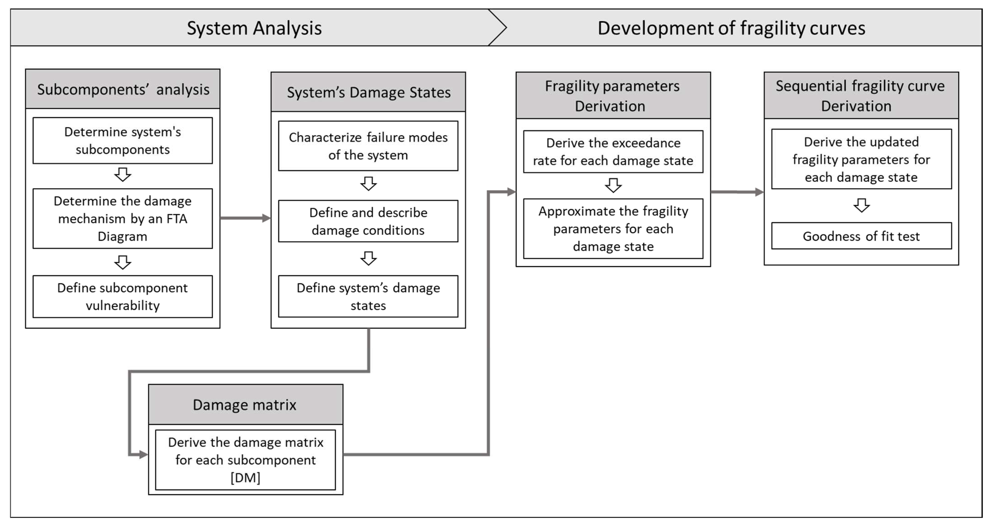
2. Methodology

Critical infrastructure is composed of several core subcomponents that are crucial for the proper operation of the system. Therefore, to develop the most representative and precise fragility curves for the system, it is proposed to develop original fragility curves based on the vulnerabilities of its subcomponents and the system failure propagation mechanisms thereof. The general methodology framework is illustrated in Figure 1.

This section presents the algorithms applied in the methodology, with the variables and indices defined in Abbreviations.

2.1. Definition of System’s Subcomponents

The decomposition process of a CI should disassemble the system into subcomponents that represent the main functionalities of the system. The decomposition process into subcomponents must be efficient. The detail of the level of the decomposition must include all the significant subcomponents, which can determine the vulnerability of the whole system. The total number of the subcomponent ${\mathrm{N}}_{\mathrm{SC}}$ is determined according to the complexity of the system and in accordance with the decision-maker policy. The index of the subcomponent is defined as $\mathrm{k} \in \left\{1,2,..,{ \mathrm{N}}_{\mathrm{SC}}\right\}$.

2.2. Definition of the Functional Relation and Damage Mechanism

The logic flow of the subcomponents illustrates the dependence of the system and the interdependencies between the different subcomponents. The relations are best demonstrated by a top-down fault tree analysis (FTA), which helps identify the system’s different failure modes and distinguishes between the different triggering failure events. The FTA scheme demonstrates the functional interrelationship of the sub-components.

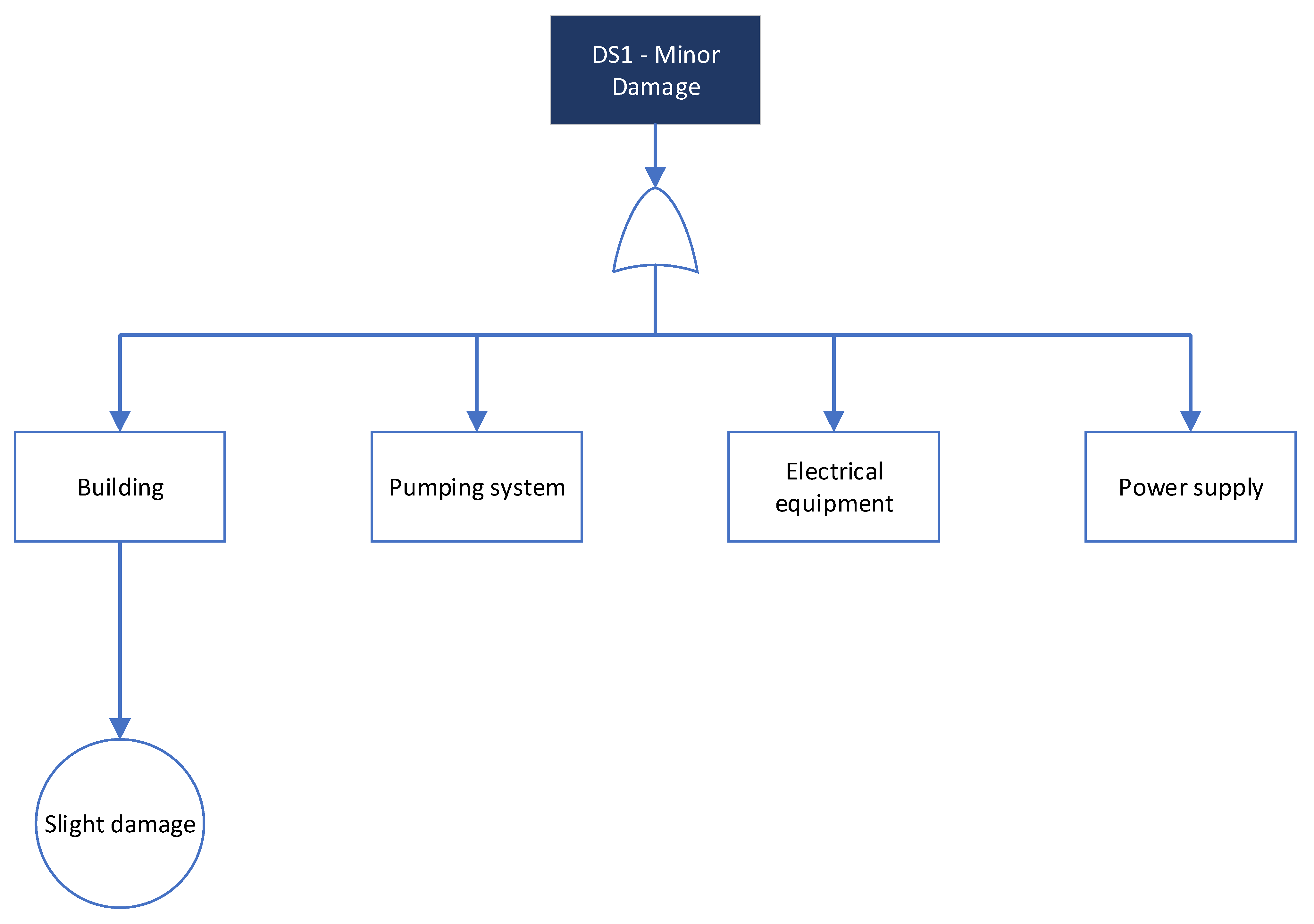
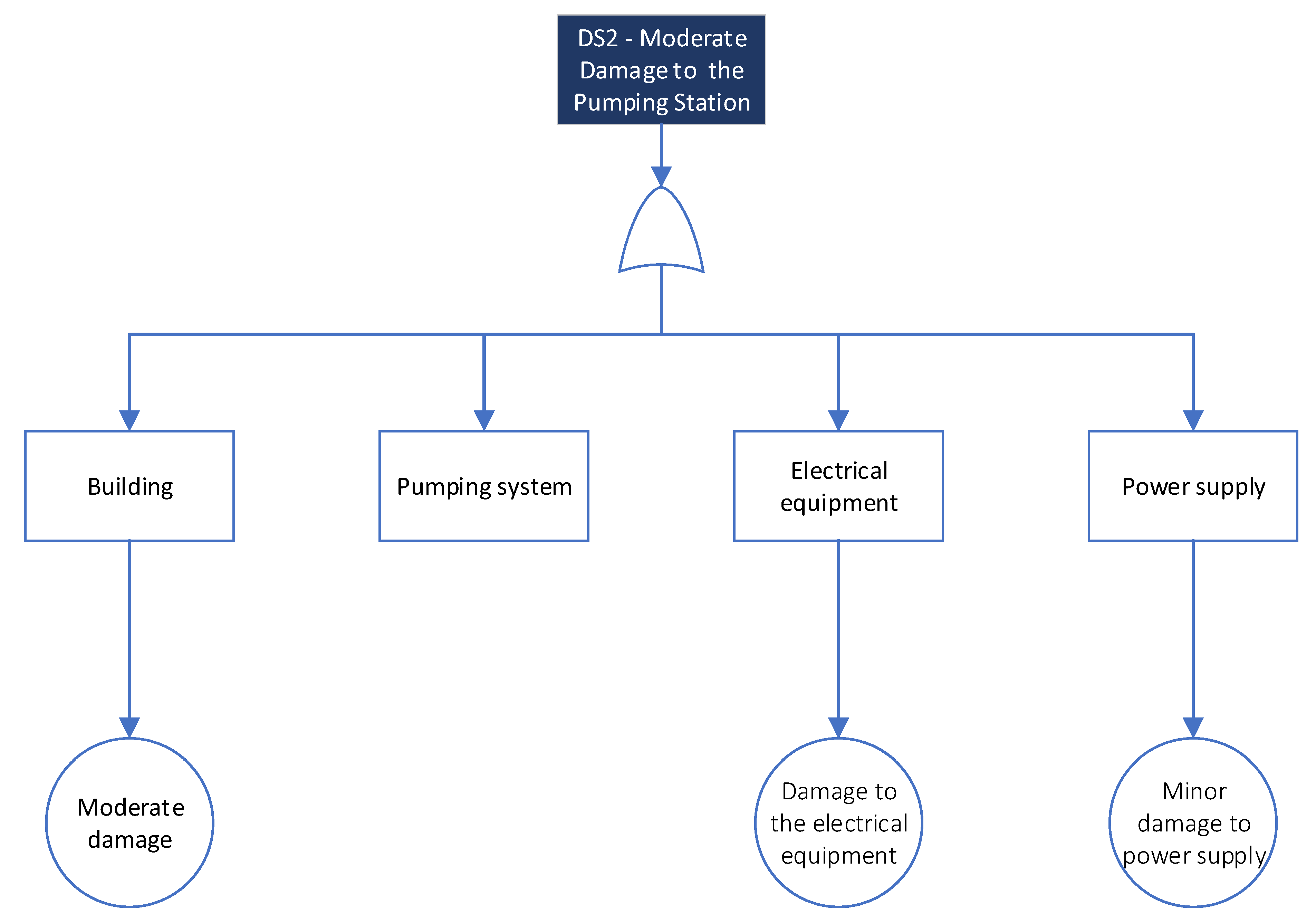
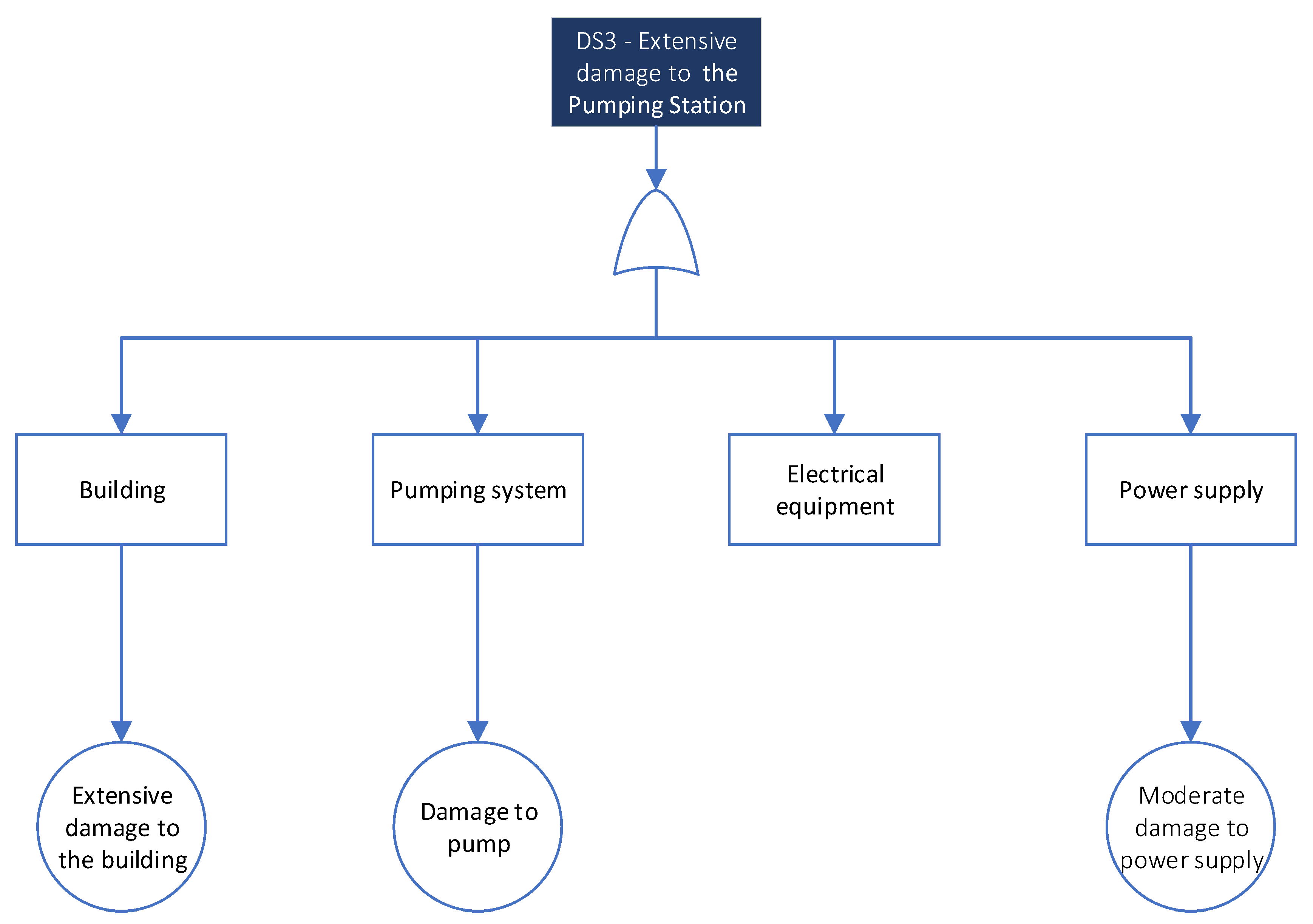
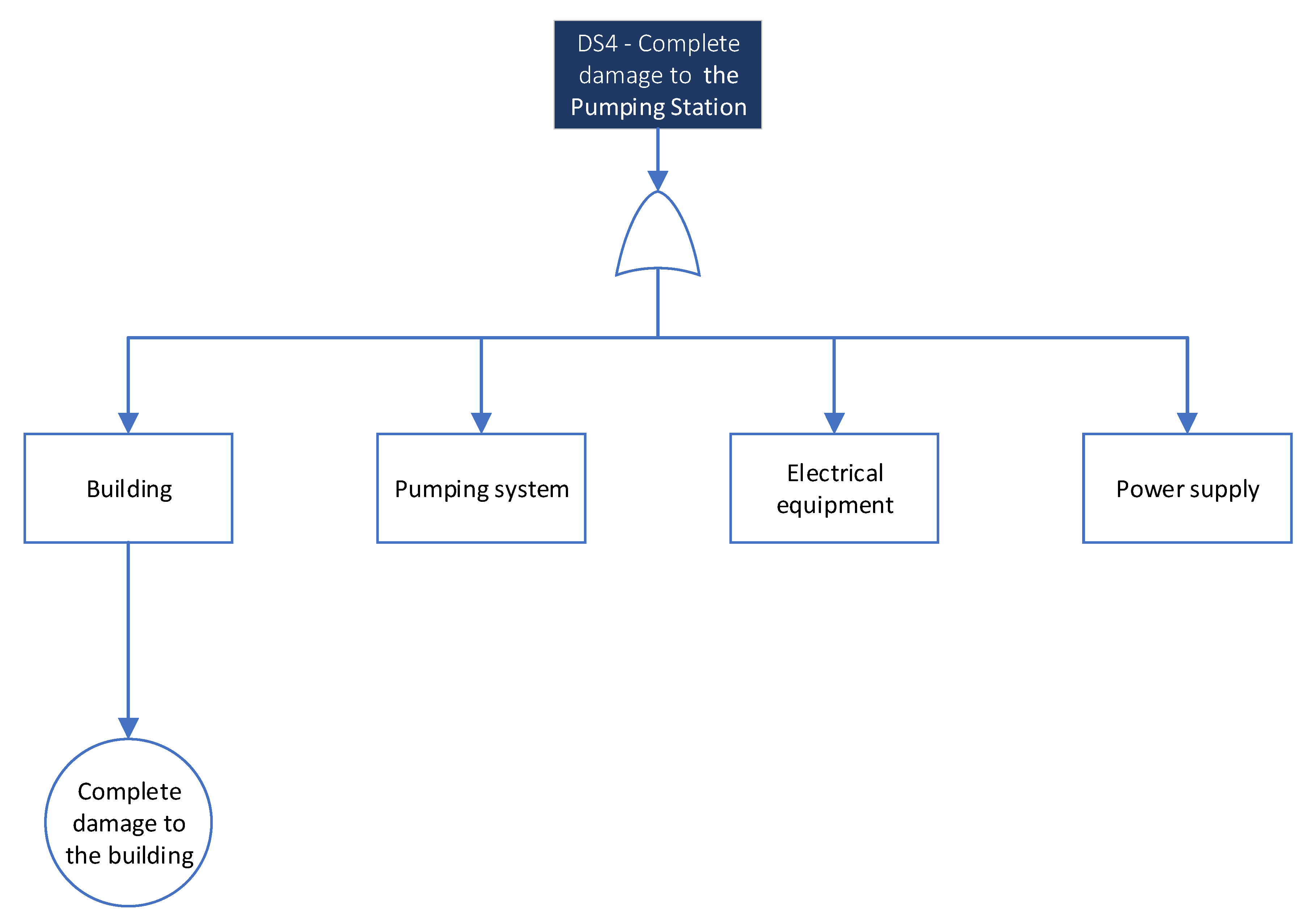
2.3. Definition of the System’s Damage States

Each damage state represents the damage and the failure mechanism severity of the CI system in terms of structural damage, functionality, performance, repair time, and costs. The damages states are ordered and defined in a sequential mode according to the severity of the failure mechanism. ${\mathrm{ds}}_{\mathrm{i}}$ represents the damage state $\mathrm{i}\in \left\{0,1,\dots ,{ \mathrm{N}}_{\mathrm{DS}}\right\}$. The definition of the damage states can be genuine and defined according to the decision-makers policies or based on known and defined parameters for common systems and components as proposed in the literature. In most cases, five damage states are defined: (ds₀) None, (ds₁) Slight damage, (ds₂) Moderate damage, (ds₃) Extensive damage, and (ds₄) Complete damage. Three main principles must be followed through the definition process and inference of the damage states:

• Degree of Severity—the damage states must reflect the expected consequences: the severity of the consequences in terms of functionality and performance of the CI system, the time required to return to the original state, and the expected economic loss (direct and indirect).
• Exclusiveness—at any time, a component can be categorized at only one damage state.
• Unambiguousness—the definition of a damage state must be exclusive, descriptive, and straightforward, i.e., for a particular observation, all its details must be concluded in the same specific damage state.

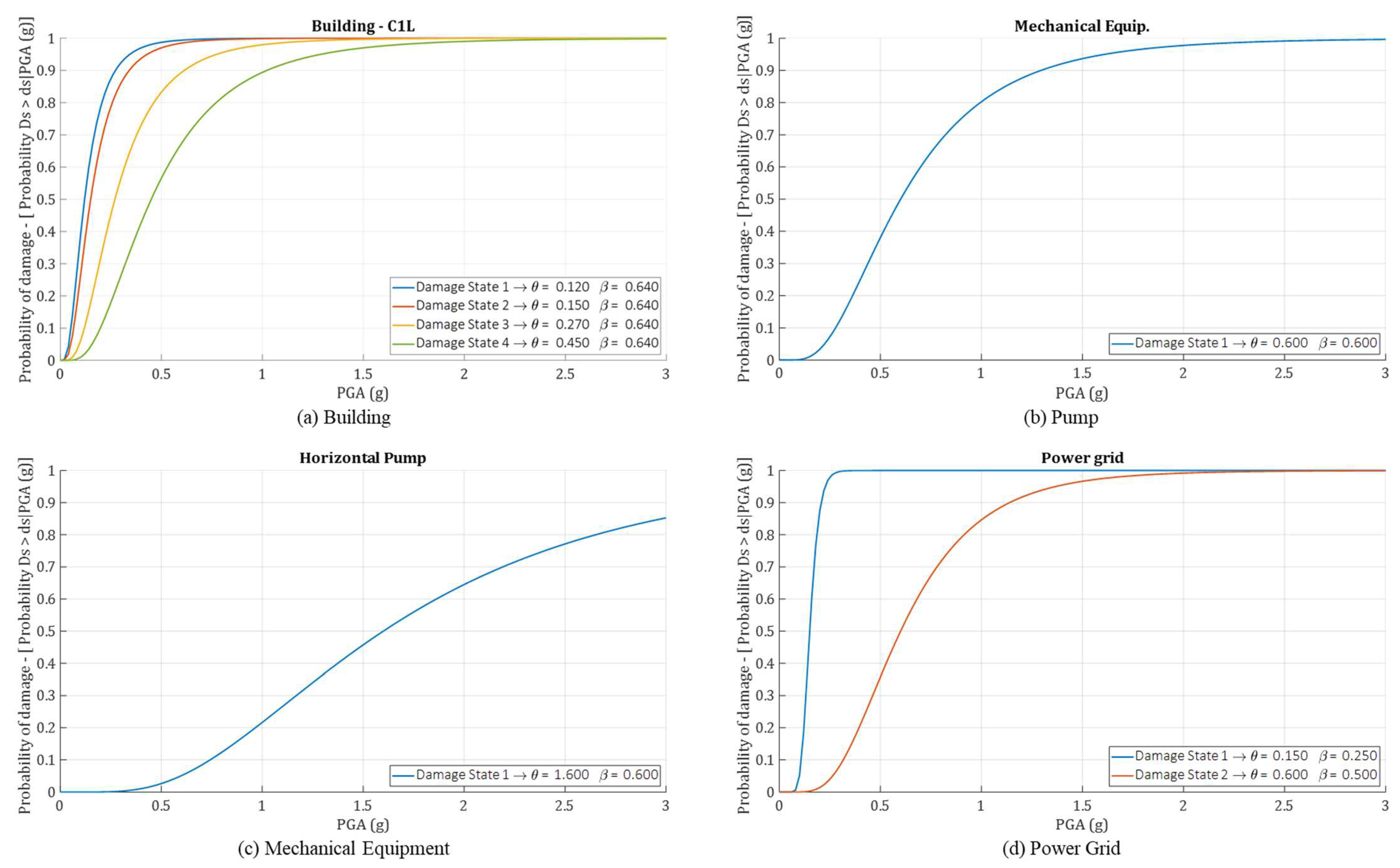
2.4. Definition of the Subcomponents’ Vulnerability

The vulnerability of the subcomponents is expressed by independent fragility curves. For each subcomponent, damage states are defined based on their vulnerability and complexity. ${\mathrm{ds}}_{\mathrm{j}}^{\mathrm{k}}$ represents the damage state $\mathrm{j}$ of the subcomponent $\mathrm{k}$ where $\mathrm{j}=0,1,\dots ,{ \mathrm{N}}_{\mathrm{DS}}^{\mathrm{k}}$. Each damage state $\mathrm{j}$ of the subcomponent $\mathrm{k}$ is defined by two parameters: ${\mathsf{\theta }}_{{\mathrm{ds}}_{\mathrm{j}}}^{\mathrm{k}}$ and ${\mathsf{\beta }}_{{\mathrm{ds}}_{\mathrm{j}}}^{\mathrm{k}}$.

The importance (i.e., the weight) of each subcomponent will be expressed in the fragility curve of the whole system. A subcomponent with high importance will have a more significant effect on the system vulnerability than an insignificant sub-component with a minor impact. Therefore, the actual weight of a component is derived according to the functional interrelation which is defined through the fault tree analysis combined with damage state definition.

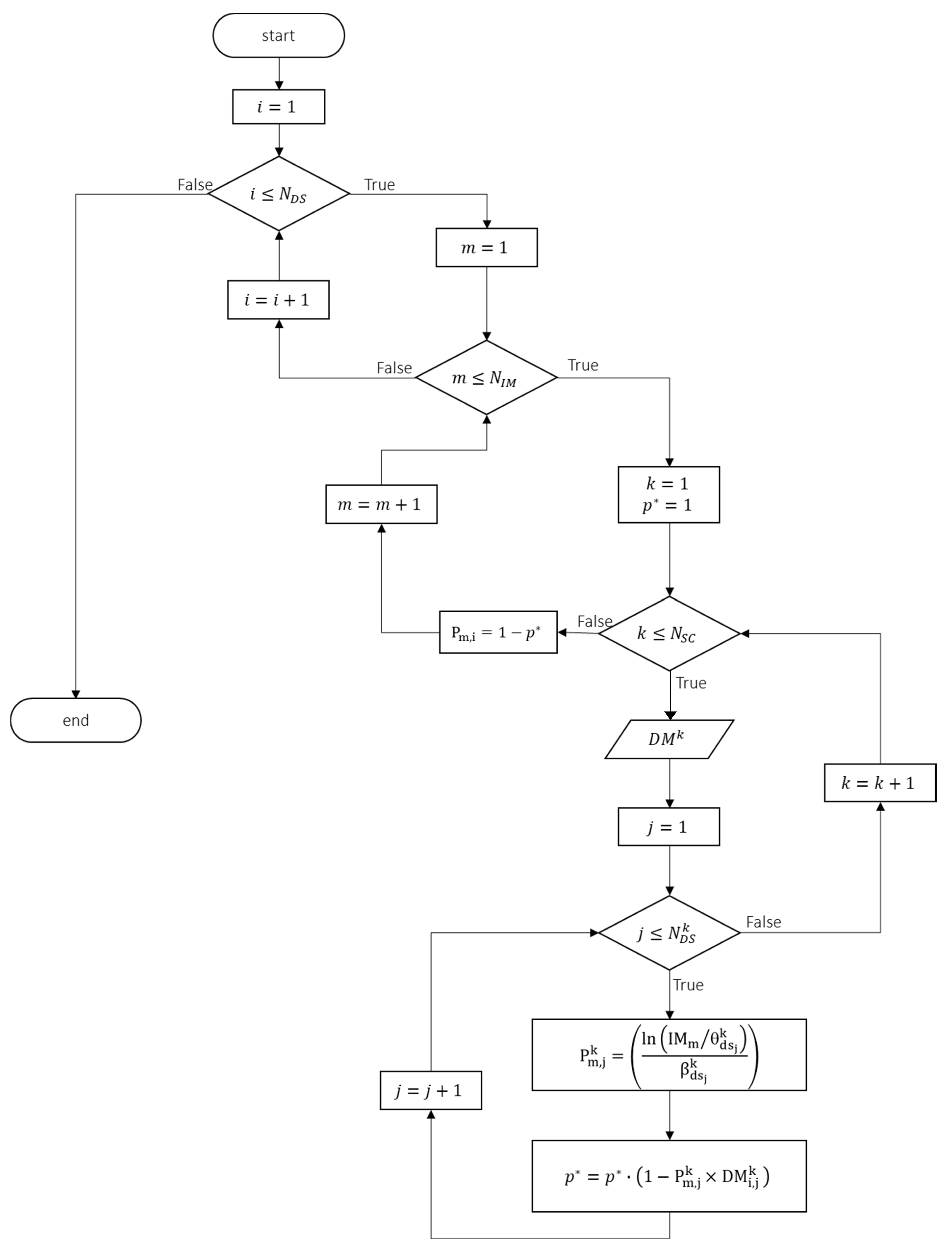
2.5. Determination of the Damage Matrix (DM)

The damage matrix ${\mathrm{DM}}^{\mathrm{k}}$ is derived for each subcomponent $\mathrm{k}$. The matrix dimensions are $\left[{\mathrm{N}}_{\mathrm{DS}}\times {\mathrm{N}}_{\mathrm{DS}}^{\mathrm{k}}\right]$ and it contains Boolean values (0 or 1). It represents whether an exceedance of the subcomponent damage state $\mathrm{j}$ will generate an exceedance of a damage state $\mathrm{i}$ of the system (1), or not (0). Equation (3) illustrates the general formulation of the damage matrix.

$${\left[\mathrm{DM}\right]}^{\mathrm{k}}=\left[{\mathrm{N}}_{\mathrm{DS}}\times {\mathrm{N}}_{\mathrm{DS}}^{\mathrm{k}}\right]={\left[\begin{array}{ccc}{\mathrm{DM}}_{1,1}& \dots & {\mathrm{DM}}_{1,{\mathrm{N}}_{\mathrm{DS}}^{\mathrm{k}}}\\ ⋮& \ddots & ⋮\\ {\mathrm{DM}}_{{\mathrm{N}}_{\mathrm{DS}},1}& \dots & {\mathrm{DM}}_{{\mathrm{N}}_{\mathrm{DS}},{\mathrm{N}}_{\mathrm{DS}}^{\mathrm{k}}}\end{array}\right]}^{\mathrm{k}}$$

(3)

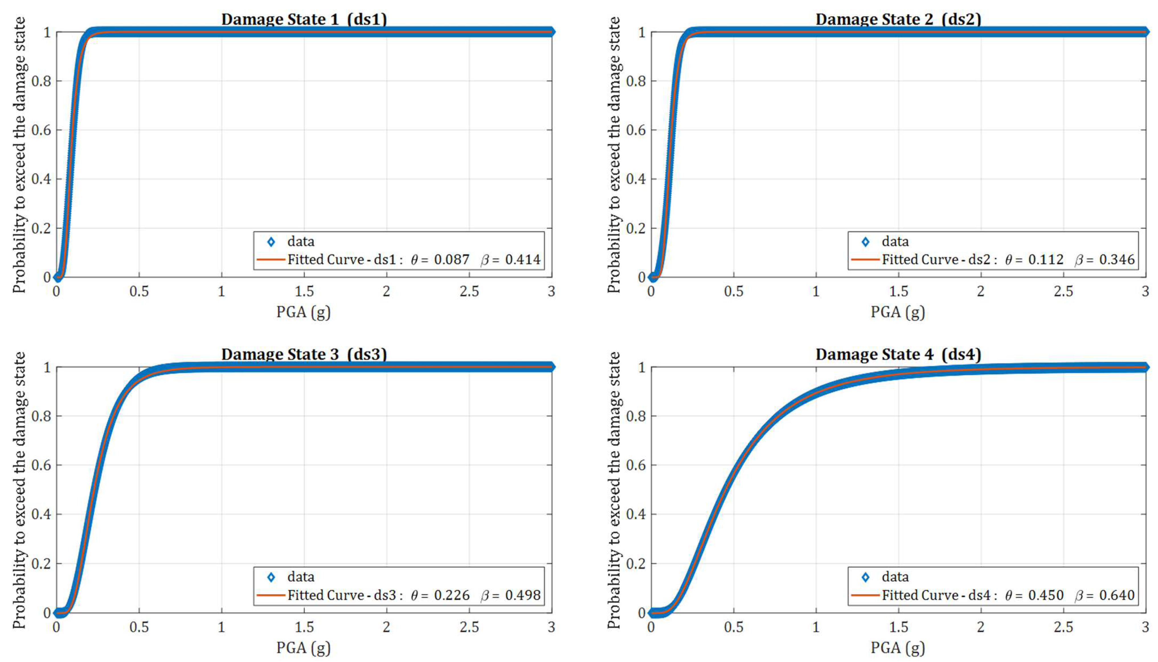
2.6. Derivation of Fragility Parameters

In this step, the CI fragility parameters of each damage state are approximated: ${\mathsf{\theta }}_{{\mathrm{ds}}_{\mathrm{i}}}$ and ${\mathsf{\beta }}_{{\mathrm{ds}}_{\mathrm{i}}}$. This step is carried out for each damage state ${\mathrm{ds}}_{\mathrm{i}}$.

2.6.1. Derivation of the Rate of Exceedance

The derivation of the rate of exceedance is performed for each damage state $\mathrm{i}$ and each IM value ${\mathrm{IM}}_{\mathrm{m}}$. This analysis combines the subcomponent fragility curves and damage matrix. The probability that a subcomponent $\mathrm{k}$ exceeds a damage state $\mathrm{j}$ is calculated for a given value of ${\mathrm{IM}}_{\mathrm{m}}$ as expressed in Equation (4).

$${\mathrm{P}}_{\mathrm{m},\mathrm{j}}^{\mathrm{k}}=\mathrm{\Phi }\left(\frac{\ln \left({\mathrm{IM}}_{\mathrm{m}}/{\mathsf{\theta }}_{{\mathrm{ds}}_{\mathrm{j}}}^{\mathrm{k}}\right)}{{\mathsf{\beta }}_{{\mathrm{ds}}_{\mathrm{j}}}^{\mathrm{k}}}\right)$$

(4)

The compounding of the system damage states is carried out by the multiplication of the subcomponent $\mathrm{k}$ damage matrix ${\mathrm{DM}}^{\mathrm{k}}$ and the failure probability for the given IM_m. Subsequently, for each damage state $\mathrm{i}$, the exceedance probability ${\mathrm{P}}_{\mathrm{m},\mathrm{i}}$ for an IM value ${\mathrm{IM}}_{\mathrm{m}}$ is derived using De-Morgan’s law for union (Equation (5)). Figure 2 depicts the flow chart of the derivation of the fragility parameters. For each damage state an ${\mathrm{N}}_{\mathrm{I}\mathrm{M}}$ simulations are executed, in each simulation, the probability of every subcomponent to exceed a certain damage state is calculated.

$${\mathrm{P}}_{\mathrm{m},\mathrm{i}}=1-{\displaystyle \prod }_{\mathrm{k}=1}^{{\mathrm{N}}_{\mathrm{SC}}}{\displaystyle \prod }_{\mathrm{j}=1}^{{\mathrm{N}}_{\mathrm{DS}}^{\mathrm{k}}}\left[1-\mathrm{\Phi }\left(\frac{\ln \left({\mathrm{IM}}_{\mathrm{m}}/{\mathsf{\theta }}_{{\mathrm{ds}}_{\mathrm{j}}}^{\mathrm{k}}\right)}{{\mathsf{\beta }}_{{\mathrm{ds}}_{\mathrm{j}}}^{\mathrm{k}}}\right)\times {\mathrm{DM}}_{\mathrm{i},\mathrm{j} }^{\mathrm{k}}\right]=1-{\displaystyle \prod }_{\mathrm{k}=1}^{{\mathrm{N}}_{\mathrm{SC}}}{\displaystyle \prod }_{\mathrm{j}=1}^{{\mathrm{N}}_{\mathrm{DS}}^{\mathrm{k}}}\left[1-{\mathrm{P}}_{\mathrm{m},\mathrm{j}}^{\mathrm{k}}\times {\mathrm{DM}}_{\mathrm{i},\mathrm{j} }^{\mathrm{k}}\right]$$

(5)

2.6.2. Approximation of Fragility Parameters—Fitting

The system’s fragility curve parameters are estimated using the exceedance rate data derived from the previous step. The input data for this process is the fraction rate of the particular damage state and its corresponding IM values. The output of this step is the estimated $\hat{\mathsf{\mu }}$ and $\hat{\mathsf{\beta }}$ that have best fit for the CDF of the fragility curve for the particular damage state. The fragility parameters are approximated, based on the log-normal CDF for each damage state using a curve fitting method (Equation (6)). Two methods are proposed for estimating the parameters by curve fitting: (1) Least-Squares Fitting (LSF) and (2) Minimizing Vector Norm (MVN).

$$\mathrm{f}\left(\mathrm{x}\right)=\mathrm{P}\left({\mathrm{DS}}_{\mathrm{i}}{ |\mathrm{IM}}_{\mathrm{m}} \right)=\mathrm{\Phi }\left(\frac{\ln \left(\mathrm{x}/{\mathsf{\theta }}_{\mathrm{ds}}{}_{\mathrm{i}}\right)}{{\mathsf{\beta }}_{{\mathrm{ds}}_{\mathrm{i}}}}\right)=\mathrm{\Phi }\left(\frac{\ln \left({\mathrm{IM}}_{\mathrm{m}}\right)-{\mathsf{\mu }}_{{\mathrm{ds}}_{\mathrm{i}}}}{{\mathsf{\beta }}_{\mathrm{ds}}{}_{\mathrm{i}}}\right)$$

(6)

2.6.3. Least-Squares Fitting (LSF)

The least-squares method minimizes the summed square of residuals. The residual for the ${\mathrm{m}}_{\mathrm{th}}$ data point ${\mathrm{r}}_{\mathrm{m}}$ is defined as the difference between the observed response value ${\mathrm{y}}_{\mathrm{i}}$ and the fitted response value $\widehat{{\mathrm{y}}_{\mathrm{m}}}$, and is identified as the error associated with the data. The summed square of residuals is stated in Equation (7).

$$\mathrm{S}={\displaystyle \sum }_{\mathrm{m}=1}^{{\mathrm{N}}_{\mathrm{IM}}}{\mathrm{r}}_{\mathrm{m}}^2={\displaystyle \sum }_{\mathrm{m}=1}^{{\mathrm{N}}_{\mathrm{IM}}}{\left({\mathrm{y}}_{\mathrm{m}}-\widehat{{\mathrm{y}}_{\mathrm{m}}}\right)}^2$$

(7)

In this procedure, the proposed method for estimating $\mathsf{\mu }$ and $\mathsf{\beta }$ is using the Least-Squares Fitting (LSF) between the analysis fraction results and probabilities of collapse predicted by Equation (8). ${\mathrm{N}}_{\mathrm{IM}}$ presents the number of IM increments and also the size of the $\mathrm{x}$ vector. The mathematical expression of the LSF problem is expressed as follows:

$$\left\{{\hat{\mathsf{\mu }}}_{\mathrm{i}}{\hat{\mathsf{\beta }}}_{\mathrm{i}}\right\}=\underset{{\mathsf{\mu }}_{\mathrm{i}}{ \mathsf{\beta }}_{\mathrm{i}}}{\min }{\displaystyle \sum }_{\mathrm{m}=1}^{{\mathrm{N}}_{\mathrm{IM}}}{\left(\mathrm{f}\left({\mathrm{IM}}_{\mathrm{m}} \right)-\hat{\mathrm{f}}\left({\mathrm{IM}}_{\mathrm{m}}\right)\right)}^2=\underset{{\mathsf{\mu }}_{\mathrm{i}}{ \mathsf{\beta }}_{\mathrm{i}}}{\min }{\displaystyle \sum }_{\mathrm{m}=1}^{\mathrm{M}}{\left({\mathrm{P}}_{\mathrm{m},\mathrm{i}}-\mathrm{\Phi }\left(\frac{\ln \left({\mathrm{IM}}_{\mathrm{m}}\right)-{\mathsf{\mu }}_{\mathrm{i}}}{{\mathsf{\beta }}_{\mathrm{i}}}\right)\right)}^2$$

(8)

2.6.4. Minimizing Vector Norm (MVN)

The MVN method estimates $\mathsf{\mu }$ and $\mathsf{\beta }$ by Minimizing the Vector Norm (MVN) for $\mathrm{p}=1$ and $\mathrm{p}=\infty .$ The IM values are represented by vector $\overrightarrow{\mathrm{x}}$ and fraction rates are represented as $\mathrm{P}{\left(\mathrm{DS}|\mathrm{IM}=\mathrm{x}\right)}_{\mathrm{data}}$. The mathematical expression of the MVN method is defined in Equation (9).

$$\left\{\widehat{{\mathsf{\mu }}_{\mathrm{i}}} \widehat{{\mathsf{\beta }}_{\mathrm{i}}}\right\}=\underset{\mathsf{\mu } \mathsf{\beta }}{\min }\mathrm{f}({\mathrm{IM}}_{\mathrm{m}},{\mathsf{\mu }}_{\mathrm{i}},{\mathsf{\beta }}_{\mathrm{i}})=\underset{\mathsf{\mu } \mathsf{\beta }}{\min }\Vert {\overrightarrow{\mathrm{f}\left({\mathrm{IM}}_{\mathrm{m}}\right)-\hat{\mathrm{f}}\left({\mathrm{IM}}_{\mathrm{m}}\right)}\Vert }_{\mathrm{p}}=\underset{\mathsf{\mu } \mathsf{\beta }}{\min }\Vert {\overrightarrow{{\mathrm{P}}_{\mathrm{m},\mathrm{i}}-\mathrm{\Phi }(\frac{\ln \left({\mathrm{IM}}_{\mathrm{m}}\right)-{\mathsf{\mu }}_{\mathrm{i}}}{{\mathsf{\beta }}_{\mathrm{i}}})}\Vert }_{\mathrm{p}}$$

(9)

2.7. Development of Sequential Fragility Curve

In order to ensure that the sequential fragility curves are not crossing each other, it is proposed to implement the following correction of the median and the logarithmic standard deviation for each damage state as proposed by [68].

$$\begin{gathered} {\mathsf{\beta }}^{\prime }=\frac{1}{{\mathrm{N}}_{\mathrm{DS}}}{\displaystyle \sum }_{\mathrm{i}=1}^{{\mathrm{N}}_{\mathrm{DS}}}{\mathsf{\beta }}_{{\mathrm{ds}}_{\mathrm{i}}} \\ {\mathsf{\theta }}_{{\mathrm{ds}}_{\mathrm{i}}}^{\prime }{=}_{{{\mathsf{\theta }}_{\mathrm{ds}}}_{\mathrm{i}}}·{\mathrm{e}}^{-0.842·\left({\mathsf{\beta }}^{\prime }-{\mathsf{\beta }}_{{\mathrm{ds}}_{\mathrm{i}}}\right)} \end{gathered}$$

(10)

The new logarithmic standard deviation ${\mathsf{\beta }}^{\prime }$ is defined and is implemented for all damage states. A common logarithmic standard deviation ensures that the fragility curves will not cross each other. ${\mathsf{\theta }}_{{\mathrm{ds}}_{\mathrm{i}}}^{\prime }$ is a new median capacity for each damage state $\mathrm{i}$. In this final step, the fragility curve parameters for each damage state are determined.

In order to validate the final values of the parameters, a goodness of fit test between the derived fragility parameters and the input data (exceedance probability) is carried out for each damage state i. The goodness of fit test is aimed to measure how well the data fits the determined fragility functions. The proposed fit test in this research is R squared when the Sum of Squares due to Error (SSE) is calculated in the following Equation (11).

$${\mathrm{SSE}}_{\mathrm{i}}={\displaystyle \sum }_{\mathrm{m}=1}^{{\mathrm{N}}_{\mathrm{IM}}}\left[{\mathrm{P}}_{\mathrm{m},\mathrm{i}}-\left(\frac{\ln \left({\mathrm{IM}}_{\mathrm{m}}/{{\mathsf{\theta }}^{\prime }}_{{\mathrm{ds}}_{\mathrm{i}}}\right)}{{\mathsf{\beta }}^{\prime }}\right)\right]$$

(11)

3. Case Study

This section presents an implementation of the methodology with a case of a generic oil pumping station facility. Pumping stations serve to maintain the flow of oil across critical pipeline systems. They are located at specific intervals along the pipeline network to ensure transport over long distances and around the storage facilities, while pressure must be maintained due to friction losses. Furthermore, pumping stations are required to transport oil uphill when topographic conditions so require.

A generic pumping station is composed of four main subcomponents that are vital for the functionality of the pumping station [69]: building, pumps, electro-mechanical equipment, and power supply. The building is usually a one-story building, in which the seismic robustness is based on the type of the building. Each station has one or more pumps (for redundancy). The pump can be categorized as horizontal or vertical, centrifugal or reciprocating type, and according to pump capacity. Electro-mechanical equipment includes equipment that is essential for the system operation, such as electric boards, end-fixtures, communication components, and computers. The power supply is usually based on the continuous supply of the external electric power grid. Additionally, in many cases, the power supply is also backed up by a diesel generator, which can be with or without seismic isolation. Failure or interruption of a pumping station is most likely to occur because of damage to one of its main subcomponents, which are vital for the continuity of performance of the station. There are limited references in the literature to post-earthquake damage to oil pumping stations [70]. The functionality of the pumping station can be corrupted due to different failures of the sub-components, such as pipe leakage or breakage, sheltering structure collapse and debris damage to equipment, damage to unanchored mechanical components, electric power supply failure due to power network disruption or due to loss of the power lines [69].

Fragility curves for pumping stations are presented in the literature [56]. However, the published fragility curves classify the pumping station only by capacity: small—less than ten m.g.d. (million gallons per day), or medium\large—more than ten m.g.d. capacity, and to an anchoring scheme of the subcomponents (special seismic tie-downs and tiebacks) or unanchored (manufactures normal requirements). This classification is very generic and does not consider characteristics that can affect the damage severity such as the number of pumps, the robustness of the building, and power supply redundancy (whether there is a backup generator). In this manuscript, the methodology for the development of exclusive fragility curves with respect to those considerations is presented. The following sections demonstrate a systematic development of the fragility curves for three possible types of pumping, which differ from each other in one of the subcomponents.

3.1. Alternative 1—Generic Pumping Station

The origin alternative is a generic pumping station without redundant components. It is composed of four subcomponents: a one-story RC moment frame building $\left(\mathrm{k}=1\right)$, one horizontal pump $\left(\mathrm{k}=2\right)$, mechanical and electrical equipment $\left(\mathrm{k}=3\right)$, and an electric power supply based on the external electric grid $\left(\mathrm{k}=4\right)$.

A failure of the pumping station or disruption to its functionality occurs due to a failure in one or more subcomponents. Based on [56,71], four damage states are defined for this pumping station, the description of each damage state is elaborated in

Table 1. Damage state description of an oil pumping station (Adapted from Refs. [56,71]).

Damage State		Damage Definition	Performance
${\mathrm{ds}}_0$	No damage		Full function
${\mathrm{ds}}_1$	Slight/minor	Defined by light damage to the building.	Full function
${\mathrm{ds}}_2$	Moderate	Defined by considerable damage to mechanical and electrical equipment, or considerable damage to the building, or loss of electric power for up to 7 days (minor damage).	Malfunction (full function after repairs)
${\mathrm{ds}}_3$	Extensive	Defined by the building being extensively damaged, or pumps badly damaged beyond repair, loss of electric power for more than 7 days (moderate damage).	Full loss of function (unrepairable damage)
${\mathrm{ds}}_4$	Complete	Defined by the building exceeding complete damage state, Pumps and electric power comprehensively damaged.

. Figure 3, Figure 4, Figure 5 and Figure 6 illustrate the FTA diagrams with the basic initiating events for each damage state.

The vulnerability of the subcomponents is expressed by distinct fragility curves. For each subcomponent $\mathrm{k}$, the number of damage states, ${\mathrm{N}}_{\mathrm{DS}}^{\mathrm{k}}$, are defined based on their vulnerability and complexity. The building is a one-story RC moment frame building which can be classified as type C1L (low-rise concrete moment frame) based on the HAZUS terminology [56]. In this case, the fragility parameters are defined based on [56,69]. Four damage states are defined for the building. One damage state is defined for the pump system (extensive) and the mechanical equipment (moderate), and two damage states are defined for the power supply (minor and moderate). The fragility parameters for each subcomponent are presented in

Table 2. Subcomponents’ fragility parameters on which values (Adapted from Ref. [56]).

	Building RC Moment Frame—Type C1L				Pump 1× Horizontal Pump	Mechanical Equipment	Power Supply External Power Grid
$\mathbf{k}$	1				2	3	4
${\mathbf{N}}_{\mathbf{D}\mathbf{S}}^{\mathbf{k}}$	${\mathbf{N}}_{\mathbf{D}\mathbf{S}}^{\mathbf{1}}=\mathbf{4}$				${\mathbf{N}}_{\mathbf{D}\mathbf{S}}^{\mathbf{2}}=\mathbf{1}$	${\mathbf{N}}_{\mathbf{D}\mathbf{S}}^{\mathbf{3}}=\mathbf{1}$	${\mathbf{N}}_{\mathbf{D}\mathbf{S}}^{\mathbf{4}}=\mathbf{2}$
$\mathbf{d}{\mathbf{s}}_{\mathbf{j}}^{\mathbf{k}}$	$\mathbf{d}{\mathbf{s}}_{\mathbf{1}}^{\mathbf{1}}$	$\mathbf{d}{\mathbf{s}}_{\mathbf{2}}^{\mathbf{1}}$	$\mathbf{d}{\mathbf{s}}_{\mathbf{3}}^{\mathbf{1}}$	$\mathbf{d}{\mathbf{s}}_{\mathbf{4}}^{\mathbf{1}}$	$\mathbf{d}{\mathbf{s}}_{\mathbf{1}}^{\mathbf{2}}$	$\mathbf{d}{\mathbf{s}}_{\mathbf{1}}^{\mathbf{3}}$	$\mathbf{d}{\mathbf{s}}_{\mathbf{1}}^{\mathbf{4}}$	$\mathbf{d}{\mathbf{s}}_{\mathbf{2}}^{\mathbf{4}}$
${\mathsf{\theta }}_{\mathbf{d}{\mathbf{s}}_{\mathbf{j}}}^{\mathbf{k}}$	$0.120$	$0.150$	$0.270$	$0.450$	$1.600$	$0.600$	$0.150$	$0.600$
${\mathsf{\mu }}_{\mathbf{d}{\mathbf{s}}_{\mathbf{j}}}^{\mathbf{k}}$	$-2.120$	$-1.897$	$-1.309$	$-0.799$	$0.470$	$-0.511$	$-1.897$	$-0.511$
${\mathsf{\beta }}_{\mathbf{d}{\mathbf{s}}_{\mathbf{j}}}^{\mathbf{k}}$	$0.640$	$0.640$	$0.640$	$0.640$	$0.600$	$0.600$	$0.250$	$0.500$

and illustrated in Figure 7.

For each subcomponent, following the damage states of the pumping station system and subcomponents’ damage states, a damage matrix $\mathrm{D}{\mathrm{M}}^{\mathrm{k}}$ is derived.

$${\left[\mathrm{D}\mathrm{M}\right]}^1=\left[\begin{array}{cccc}1& 0& 0& 0\\ 0& 1& 0& 0\\ 0& 0& 1& 0\\ 0& 0& 0& 1\end{array}\right], {\left[\mathrm{D}\mathrm{M}\right]}^2=\left[\begin{array}{c}0\\ 0\\ 1\\ 0\end{array}\right] , {\left[\mathrm{D}\mathrm{M}\right]}^3=\left[\begin{array}{c}0\\ 1\\ 0\\ 0\end{array}\right] , {\left[\mathrm{D}\mathrm{M}\right]}^4=\left[\begin{array}{cc}0& 0\\ 1& 0\\ 0& 1\\ 0& 0\end{array}\right]$$

The selected intensity measure is PGA, and the maximum IM (${\mathrm{IM}}_{\max }$) value was determined as 3.00 (g). The number of intensities (${\mathrm{N}}_{\mathrm{IM}}$) was defined as $3000$, with an interval of $0.001$ (g). Then, for each damage state $\mathrm{i}$, the exceedance probability ${\mathrm{P}}_{\mathrm{m},\mathrm{i}}$ for an IM value of ${\mathrm{IM}}_{\mathrm{m}}$ is calculated following Equation (5). The fitted fragility curves were derived according to Equations (9) and (10). The exceedance data for each damage state $\mathrm{i}$ and the fitted parameters are illustrated in Figure 8.

The sequential fragility parameters are derived according to Equation (11). The results are detailed in

Table 3. Fragility parameters of the sequential damage states.

$\mathbf{d}{\mathbf{s}}_{\mathbf{i}}$	$\mathbf{d}{\mathbf{s}}_{\mathbf{1}}$	$\mathbf{d}{\mathbf{s}}_{\mathbf{2}}$	$\mathbf{d}{\mathbf{s}}_{\mathbf{3}}$	$\mathbf{d}{\mathbf{s}}_{\mathbf{4}}$
${\mathsf{\theta }}_{\mathrm{d}{\mathrm{s}}_{\mathrm{i}}}$	$0.085$	$0.103$	$0.235$	$0.527$
${\mathsf{\mu }}_{\mathrm{d}{\mathrm{s}}_{\mathrm{i}}}$	$-2.471$	$-2.273$	$-1.446$	$-0.640$
${\mathsf{\sigma }}_{\mathrm{d}{\mathrm{s}}_{\mathrm{i}}}$	$0.547$	$0.547$	$0.547$	$0.547$

and Figure 9.

In the present case, it is evident that the final fragility curves have been affected mostly by the building’s vulnerability, particularly in the severe damage states: $\mathrm{d}{\mathrm{s}}_3$ and $\mathrm{d}{\mathrm{s}}_4$. This finding is compatible with the conclusions that were found in [57].

In the last step, the R squared test was performed to examine how well the derived fragility curves fit the data of the rate of exceedance. The results show a high correlation for all damage states: 0.9933 for ${\mathrm{ds}}_1$, 0.9831 for ${\mathrm{ds}}_2$, 0.9966 for ${\mathrm{ds}}_3$, and 0.979 for ${\mathrm{ds}}_4$.

3.2. Alternative 2—Addition of Backup Generator

In this example, a backup diesel generator is added to increase the redundancy of the power supply. In this case, the backup generator is a diesel generator with a capacity of 350 to 750 kVA with vibration isolation. The fragility parameters are based on [72], as illustrated in Figure 10.

The additional generator increases the redundancy of the power supply. In this case, a failure of the ongoing power supply will occur only in the case of concurrent failure of the external power grid and the backup generator (Figure 11). Thus, the previous vulnerability that was represented by the subcomponent fragility curves has changed. The composite of the generator and the electric grid yields new fragility curves for the power supply subcomponent. The median of ${\mathrm{ds}}_1$ and the median of ${\mathrm{ds}}_2$ have significantly increased, as illustrated by a comparison with the previous fragility curves of the power supply (Figure 12).

Following the updated fragility parameters of the power supply, the rest of the fragility development process is similar to the first example. The derived fragility curves of the pumping station that includes a backup generator are presented in Figure 13.

3.3. Alternative 3—RC Shear Walls Building

In this case, a different type of building is examined as an alternative to increase the building’s robustness to reduce the system’s vulnerability. For this purpose, the RC moment frame building is replaced by an RC shear wall building. According to [56], this type is categorized as C2L (low-rise reinforced concrete shear walls building), the fragility parameters for this type of building are described and compared to C1L in Figure 14. Following the proposed methodology, the updated parameters for the building subcomponent and the exclusive fragility curves for the pumping station were developed (Figure 15).

3.4. Summary and Discussion

In this section, three sets of fragility curves were developed for each pumping station alternative layout. Each change in one of the subcomponents altered the final fragility curve parameters of the pumping station (

Table 4. Derived median values (${\mathsf{\theta }}_{\mathrm{ds}}{}_{\mathrm{i}}$) for each alternative of pumping station layout.

	$\mathbf{d}{\mathbf{s}}_{\mathbf{1}}$	$\mathbf{d}{\mathbf{s}}_{\mathbf{2}}$	$\mathbf{d}{\mathbf{s}}_{\mathbf{3}}$	$\mathbf{d}{\mathbf{s}}_{\mathbf{4}}$
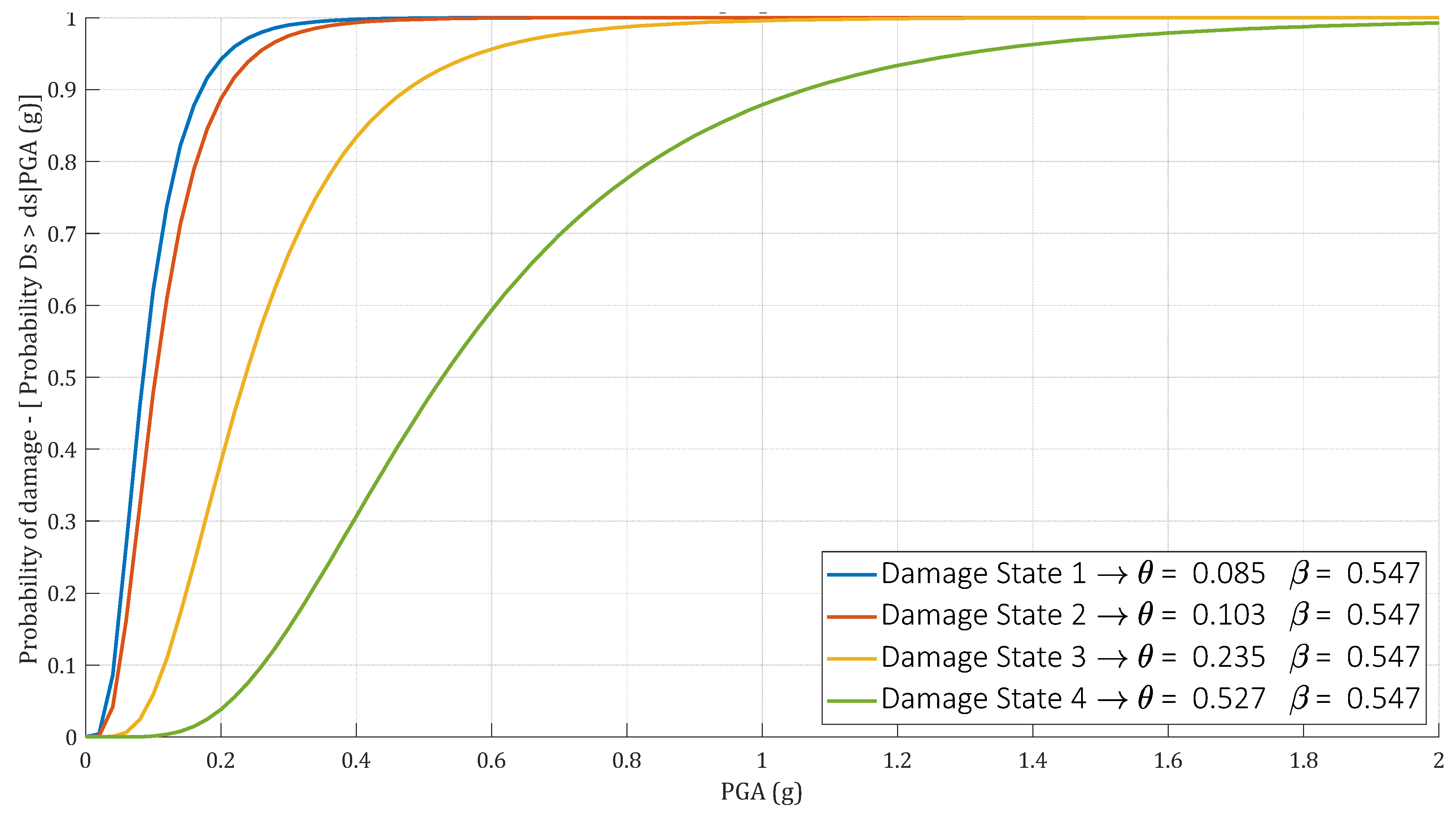
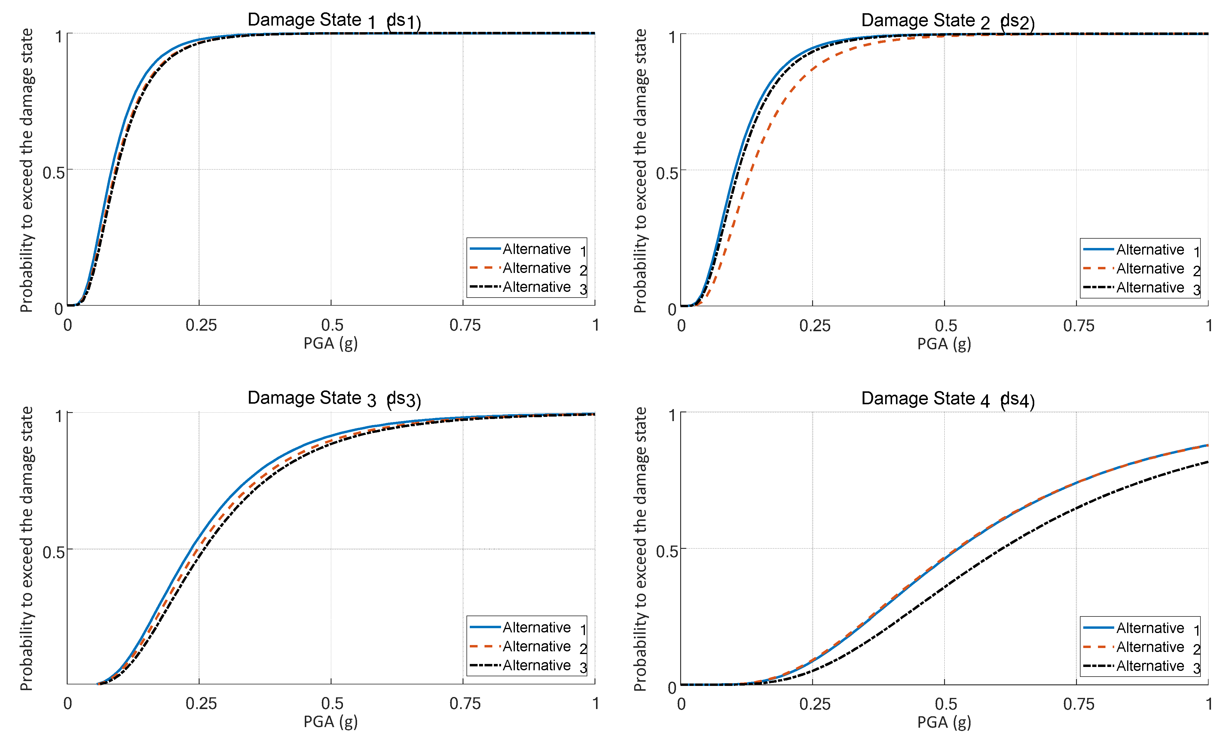
Alternative 1	0.085	0.103	0.235	0.527
Alternative 2	0.092	0.134	0.248	0.524
Alternative 3	0.094	0.110	0.260	0.611

). As a reference to the first alternative of the pumping station (i.e., generic pumping station), the addition of a backup generator (alternative 2) produced a moderate increase in the median parameters of DS₁ (+8.6%) and DS₃ (+5.15%), and a significant increase in DS₂ (+30.1%). However, a backup generator had a negligible effect on DS₄ (−0.56%) that was caused due to the sequential fragility mechanism. Those results correspond with the damage states’ description, where DS₄ is exceeded solely by complete damage to the building.

The alteration of the building type (alternative 3) to a more seismic-robust structure affects all damage states and increases the median parameters: DS₁ (+11.54%), DS₂ (+6.81%), DS₃ (+10.31%), and DS₄ (+15.77%). Thus, the pumping station vulnerability of this design alternative is mitigated.

The main highlight that was illustrated by the results is that each subcomponent has an effect on the final values of the fragility curve parameters as demonstrated in Figure 16.

The marginal contribution of each retrofit alternative is derived from the fragility curves and expressed in the risk. The difference between the median value of each alternative has implications for the effectiveness of the alternative design. For example, an additional generator increases the median value of ds₂ by over 30%, i.e., for the same IM value, the probability of exceeding ds₂ is lower, which indicates the high effectiveness of decreasing the vulnerability of the system to moderate damage state (ds₂).

4. Conclusions

A comprehensive methodology for deriving original fragility curves for CI is presented in this paper. The methodology follows a seven-step analytical procedure: (1) Definition of the system’s subcomponents, (2) Definition of damage mechanisms, (3) Definition of the system’s damage states, (4) Definition of the subcomponents’ vulnerability, (5) Determination of damage matrix, (6) Derivation of fragility parameters, and (7) Development of sequential fragility curves.

This paper presents the implementation of the methodology through a case study of a generic oil pumping station. The case study presents three alternatives of a pumping station layout that varies by different subcomponents. For each alternative, the failure mechanisms were examined, and exclusive fragility curves were developed. The derived fragility parameters differed between the alternatives, corresponding to the diverse layout of the subcomponent. The differing fragility parameters of each alternative are compatible with the assumption that each subcomponent of the critical infrastructure system can significantly affect the fragility parameters. Moreover, the variances between the damage states’ fragility parameters have implications for the effectiveness of each alternative to resist different levels of severity, relative to a reference alternative. For example, it was found that the addition of a backup diesel generator is effective in decreasing the probability of moderate damage (ds₂) while increasing the building robustness is effective for all damage states.

Many studies offered generic fragility curves for systems and components that are based on prior definitions of the system’s components and damage states, as discussed in Section 2, without consideration of the system’s unique configuration. This study, however, presents a model for developing exclusive fragility curves for critical infrastructure systems. Fragility curves are commonly used for seismic risk analysis, but the generic fragility parameters that are available in the literature are not accurate enough for their in-depth development. Therefore, in these cases, it is proposed to follow the methodology presented in this paper to develop exclusive fragility curves that reflect the actual system at high reliability. The usage of exclusive fragility curves allows us to examine actual systems for risk appraisal and risk management. Moreover, this methodology allows for the examination of the impact of each subcomponent on the whole system’s fragility curve. In addition, the proposed methodology is conceived to adjust and define the damage state based on the actual performance of the design demands and policies of the decision-makers.

This paper presents the phases of the methodology, enabling the development of the fragility curves in a systematic way. The methodology allows us to select the level of accuracy required in the risk analysis process, i.e., up to the level of detail to which the subcomponents are required to be defined. Moreover, the level of detail can be different between the subcomponents. The presented case study illustrated the decomposition of an oil pumping station into four main subcomponents that initiated the main events in the analysis of the system’s failure mechanisms. However, if a more detailed analysis is required, an additional level of decomposition might be performed.

The methodology allows us to derive fragility curves by a hybrid approach that aggregates empirical with analytical data. One can derive an exclusive fragility curve based on both empirical and analytical parameters to define the subcomponents’ vulnerability in order to compensate for the insufficiency of data of some of the components.

In the presented case study, the sub-components’ fragility curves were all based on PGA. When the subcomponents of the system require different IM parameters (or EDP—Engineering Demand Parameter), the methodology must aggregate the vulnerability of the system corresponding to each sub-component IM parameter. In those cases, it is required to use multiple hazard curves (one for each IM parameter) or to define a function that predicts the relationship between the different IM parameters. Furthermore, in order to execute the methodology, all components’ vulnerability data is required. In case of unavailable fragility curves for a specific component, it will be required to define the component’s vulnerability according to empirical data, analytical methods or according to experts’ judgement. Based on the proposed methodology for developing fragility curves, further research for seismic risk appraisal and management is intended to be produced. Using the presented procedure, it is possible to appraise the seismic risk of critical infrastructure systems and examine the effectiveness of possible retrofit alternatives, based on the level of risk mitigation. Further information for possible retrofit strategies can be found in [73,74,75,76]. In addition, this procedure can be applied in other research for developing fragility curves for critical infrastructure systems and for validation and refinement of published fragility curves.

Furthermore, fragility curves estimate the level of damage as a result of a single seismic event (i.e., mainshock) and do not consider sequential seismic events and aftershock. Studies such as [77,78] examine the impacts of aftershock events and the expected damage to the structure that has already experienced a seismic event. Further research that is implementing the presented methodology can investigate and develop fragility curves for CI systems that estimate the expected damage for aftershock and set of several seismic events.

This paper presented an original methodology for developing exclusive fragility curves for critical infrastructures by decomposition of the system into subcomponents and a Fault Tree Analysis to determine the failure mechanisms of the system. The developed fragility curves reflect the actual layout of the critical infrastructure design alternative and consider the vulnerability of the composing subcomponents.

References

- Crespi, P.; Zucca, M.; Longarini, N.; Giordano, N. Seismic Assessment of Six Typologies of Existing RC Bridges. Infrastuctures 2020, 5, 52. [Google Scholar] [CrossRef]
- Urlainis, A.; Ornai, D.; Levy, R.; Vilnay, O.; Shohet, I.M. Loss and Damage Assessment in Critical Infrastructures Due to Extreme Events. Saf. Sci. 2022, 147, 105587. [Google Scholar] [CrossRef]
- Urlainis, A.; Shohet, I.M.; Levy, R.; Ornai, D.; Vilnay, O. Damage in Critical Infrastructures Due to Natural and Man-Made Extreme Events—A Critical Review. Procedia Eng. 2014, 85, 529–535. [Google Scholar] [CrossRef]
- Sucuoğlu, H.; Akkar, S. Basic Earthquake Engineering: From Seismology to Analysis and Design; Springer: New York, NY, USA, 2013; ISBN 9783319010267. [Google Scholar]
- Grünthal, G. European Macroseismic Scale 1998; European Seismological Commission: Bucharest, Romania, 1998; ISBN 2-87977-008-4. [Google Scholar]
- Wood, H.O.; Neumann, F. Modified Mercalli Intensity Scale of 1931. Bull. Seismol. Soc. Am. 1931, 21, 277–283. [Google Scholar] [CrossRef]
- Dewey, J.W.; Reagor, B.G.; Dengler, L.; Moley, K. Intensity Distribution and Isoseismal Maps for the Northridge, California; U.S. Geological Survey: Reston, VA, USA, 1995. [CrossRef]
- Wei, H.-H.; Shohet, I.M.; Skibniewski, M.J.; Shapira, S.; Yao, X. Assessing the Lifecycle Sustainability Costs and Benefits of Seismic Mitigation Designs for Buildings. J. Archit. Eng. 2016, 22, 4015011. [Google Scholar] [CrossRef]
- Afrouz, S.G.; Farzampour, A.; Hejazi, Z.; Mojarab, M. Evaluation of Seismic Vulnerability of Hospitals in the Tehran Metropolitan Area. Buildings 2021, 11, 54. [Google Scholar] [CrossRef]
- Dolce, M.; Prota, A.; Borzi, B.; da Porto, F.; Lagomarsino, S.; Magenes, G.; Moroni, C.; Penna, A.; Polese, M.; Speranza, E.; et al. Seismic Risk Assessment of Residential Buildings in Italy. Bull. Earthq. Eng. 2021, 19, 2999–3032. [Google Scholar] [CrossRef]
- Flenga, M.G.; Favvata, M.J. Fragility Curves and Probabilistic Seismic Demand Models on the Seismic Assessment of RC Frames Subjected to Structural Pounding. Appl. Sci. 2021, 11, 8253. [Google Scholar] [CrossRef]
- Porter, K.; Kennedy, R.; Bachman, R. Creating Fragility Functions for Performance-Based Earthquake Engineering. Earthq. Spectra 2007, 23, 471–489. [Google Scholar] [CrossRef]
- Porter, K.; Hamburger, R.; Kennedy, R. Practical Development and Application of Fragility Functions. In Proceedings of the Structural Engineering Research Frontiers at Structures Congress 2007, Long Beach, CA, USA, 16–19 May 2007. [Google Scholar]
- Baker, J.W. Efficient Analytical Fragility Function Fitting Using Dynamic Structural Analysis. Earthq. Spectra 2015, 31, 579–599. [Google Scholar] [CrossRef]
- O’Rourke, M.J.; So, P. Seismic Fragility Curves for On-Grade Steel Tanks. Earthq. Spectra 2000, 16, 801–815. [Google Scholar] [CrossRef]
- Razzaghi, M.S.; Eshghi, S. Probabilistic Seismic Safety Evaluation of Precode Cylindrical Oil Tanks. J. Perform. Constr. Facil. 2015, 29, 04014170. [Google Scholar] [CrossRef]
- Rossetto, T.; Ioannou, I.; Grant, D.N. Existing Empirical Fragility and Vulnerability Functions: Compendium and Guide for Selection; Technical Report 2015-1; GEM Foundation: Pavia, Italy, 2015. [Google Scholar] [CrossRef]
- Ruggieri, S.; Tosto, C.; Rosati, G.; Uva, G.; Ferro, G.A. Seismic Vulnerability Analysis of Masonry Churches in Piemonte after 2003 Valle Scrivia Earthquake: Post-Event Screening and Situation 17 Years Later. Int. J. Archit. Herit. 2020, 16, 717–745. [Google Scholar] [CrossRef]
- Rosti, A.; del Gaudio, C.; Rota, M.; Ricci, P.; di Ludovico, M.; Penna, A.; Verderame, G.M. Empirical Fragility Curves for Italian Residential RC Buildings. Bull. Earthq. Eng. 2021, 19, 3165–3183. [Google Scholar] [CrossRef]
- Rosti, A.; Rota, M.; Penna, A. Empirical Fragility Curves for Italian URM Buildings. Bull. Earthq. Eng. 2021, 19, 3057–3076. [Google Scholar] [CrossRef]
- Biglari, M.; Formisano, A.; Hashemi, B.H. Empirical Fragility Curves of Engineered Steel and RC Residential Buildings after Mw 7.3 2017 Sarpol-e-Zahab Earthquake. Bull. Earthq. Eng. 2021, 19. [Google Scholar] [CrossRef]
- Buratti, N.; Minghini, F.; Ongaretto, E.; Savoia, M.; Tullini, N. Empirical Seismic Fragility for the Precast RC Industrial Buildings Damaged by the 2012 Emilia (Italy) Earthquakes. Earthq. Eng. Struct. Dyn. 2017, 46, 2317–2335. [Google Scholar] [CrossRef]
- Berahman, F.; Behnamfar, F. Seismic Fragility Curves for Un-Anchored on-Grade Steel Storage Tanks: Bayesian Approach. J. Earthq. Eng. 2007, 11, 166–192. [Google Scholar] [CrossRef]
- Rahmani, A.Y.; Bourahla, N.; Bento, R.; Badaoui, M. An Improved Upper-Bound Pushover Procedure for Seismic Assessment of High-Rise Moment Resisting Steel Frames. Bull. Earthq. Eng. 2018, 16. [Google Scholar] [CrossRef]
- Belejo, A.; Bento, R. Improved Modal Pushover Analysis in Seismic Assessment of Asymmetric Plan Buildings under the Influence of One and Two Horizontal Components of Ground Motions. Soil Dyn. Earthq. Eng. 2016, 87, 1–15. [Google Scholar] [CrossRef]
- Amin, J.; Gondaliya, K.; Mulchandani, C. Assessment of Seismic Collapse Probability of RC Shaft Supported Tank. Structures 2021, 33, 2639–2658. [Google Scholar] [CrossRef]
- O’Rourke, M. Analytical Fragility Relation for Buried Segmented Pipe. In Proceedings of the Technical Council on Lifeline Earthquake Engineering Conference (TCLEE), Oakland, CA, USA, 28 June–1 July 2009. [Google Scholar]
- Rabi, R.R.; Bianco, V.; Monti, G. Mechanical-Analytical Soil-Dependent Fragility Curves of Existing Rc Frames with Column-Driven Failures. Buildings 2021, 11, 278. [Google Scholar] [CrossRef]
- Güneş, N.; Ulucan, Z. Collapse probability of code-based design of a seismically isolated reinforced concrete building. Structures 2021, 33, 2402–2412. [Google Scholar] [CrossRef]
- Khorami, M.; Khorami, M.; Motahar, H.; Alvansazyazdi, M.; Shariati, M.; Jalali, A.; Tahir, M.M. Evaluation of the Seismic Performance of Special Moment Frames Using Incremental Nonlinear Dynamic Analysis. Struct. Eng. Mech. 2017, 63, 259–268. [Google Scholar] [CrossRef]
- Pourreza, F.; Mousazadeh, M.; Basim, M.C. An efficient method for incorporating modeling uncertainties into collapse fragility of steel structures. Struct. Saf. 2020, 88, 102009. [Google Scholar] [CrossRef]
- Kildashti, K.; Mirzadeh, N.; Samali, B. Seismic vulnerability assessment of a case study anchored liquid storage tank by considering fixed and flexible base restraints. Thin Walled Struct. 2018, 123, 382–394. [Google Scholar] [CrossRef]
- Razzaghi, M.S.; Eshghi, S. Development of Analytical Fragility Curves for Cylindrical Steel Oil Tanks. In Proceedings of the 14th World Conference on Earthquake Engineering, Beijing, China, 12–17 October 2008; p. 8. [Google Scholar]
- Lagomarsino, S.; Giovinazzi, S. Macroseismic and mechanical models for the vulnerability and damage assessment of current buildings. Bull. Earthq. Eng. 2006, 4, 415–443. [Google Scholar] [CrossRef]
- Jaiswal, K.S.; Aspinall, W.; Perkins, D.; Wald, D.J.; Porter, K.A. Use of Expert Judgment Elicitation to Estimate Seismic Vulnerability of Selected Building Types. In Proceedings of the 15th World Conference on Earthquake Engineering, Lisbon, Portugal, 24–28 September 2012; p. 10. [Google Scholar]
- Mosleh, A.; Apostolakis, G. The Assessment of Probability Distributions from Expert Opinions with an Application to Seismic Fragility Curves. Risk Anal. 1986, 6, 447–461. [Google Scholar] [CrossRef]
- Tafti, M.F.; Hosseini, K.A.; Mansouri, B. Generation of new fragility curves for common types of buildings in Iran. Bull. Earthq. Eng. 2020, 18, 3079–3099. [Google Scholar] [CrossRef]
- Kappos, A.J.; Panagopoulos, G.; Panagiotopoulos, C.; Penelis, G. A hybrid method for the vulnerability assessment of R/C and URM buildings. Bull. Earthq. Eng. 2006, 4, 391–413. [Google Scholar] [CrossRef]
- Kappos, A.; Pitilakis, K.; Stylianidis, K.; Morfidis, K.; Asimakopoulos, D.; Asimakopoulos, N. Cost-Benefit Analysis for the Seismic Rehabilitation of Buildings in Thessaloniki, Bases on a Hybrid Method of Vulnerability Assessment. In Proceedings of the Fifth International Conference on Seismic Zonation, Nice, France, 17–19 October 1995; pp. 406–413. [Google Scholar]
- Kappos, A.J. An overview of the development of the hybrid method for seismic vulnerability assessment of buildings. Struct. Infrastruct. Eng. 2016, 12, 1573–1584. [Google Scholar] [CrossRef]
- Polese, M.; Marcolini, M.; Zuccaro, G.; Cacace, F. Mechanism based assessment of damage-dependent fragility curves for RC building classes. Bull. Earthq. Eng. 2014, 13, 1323–1345. [Google Scholar] [CrossRef]
- Karimi-Moridani, K.; Zarfam, P.; Ghafory-Ashtiany, M. A Novel and Efficient Hybrid Method to Develop the Fragility Curves of Horizontally Curved Bridges. KSCE J. Civ. Eng. 2019, 24, 508–524. [Google Scholar] [CrossRef]
- Cardone, D.; Rossino, M.; Gesualdi, G. Estimating fragility curves of pre-70 RC frame buildings considering different performance limit states. Soil Dyn. Earthq. Eng. 2018, 115, 868–881. [Google Scholar] [CrossRef]
- Leggieri, V.; Ruggieri, S.; Zagari, G.; Uva, G. Appraising seismic vulnerability of masonry aggregates through an automated mechanical-typological approach. Autom. Constr. 2021, 132, 103972. [Google Scholar] [CrossRef]
- Lanzano, G.; Salzano, E.; de Magistris, F.S.; Fabbrocino, G. Seismic vulnerability of natural gas pipelines. Reliab. Eng. Syst. Saf. 2013, 117, 73–80. [Google Scholar] [CrossRef]
- O’Rourke, M.; Ayala, G. Pipeline Damage Due to Wave Propagation. J. Geotech. Eng. 1993, 119, 1490–1498. [Google Scholar] [CrossRef]
- Kaynia, A.; Iervolino, I.; Taucer, F.; Hancilar, U. Guidelines for Deriving Seismic Fragility Functions of Elements at Risk: Buildings, Lifelines, Transportation Networks and Critical Facilities, SYNER-G Reference Report 4; Publications Office of the European Union: Luxembourg, 2013. [Google Scholar]
- Pineda-Porras, O.; Najafi, M. Seismic Damage Estimation for Buried Pipelines: Challenges after Three Decades of Progress. J. Pipeline Syst. Eng. Pr. 2010, 1, 19–24. [Google Scholar] [CrossRef]
- Piccinelli, R.; Krausmann, E. Analysis of Natech Risk for Pipelines: A Review; Publications Office of the European Union: Luxembourg, 2013; ISBN 978-92-79-34813-6. [Google Scholar]
- Yum, S.-G.; Kim, J.-M.; Wei, H.-H. Development of vulnerability curves of buildings to windstorms using insurance data: An empirical study in South Korea. J. Build. Eng. 2020, 34, 101932. [Google Scholar] [CrossRef]
- Baker, J.W.; Cornell, C.A. A vector-valued ground motion intensity measure consisting of spectral acceleration and epsilon. Earthq. Eng. Struct. Dyn. 2005, 34, 1193–1217. [Google Scholar] [CrossRef]
- Lallemant, D.; Kiremidjian, A.; Burton, H. Statistical procedures for developing earthquake damage fragility curves. Earthq. Eng. Struct. Dyn. 2015, 44, 1373–1389. [Google Scholar] [CrossRef]
- Zentner, I.; Gündel, M.; Bonfils, N. Fragility analysis methods: Review of existing approaches and application. Nucl. Eng. Des. 2017, 323, 245–258. [Google Scholar] [CrossRef]
- Baltzopoulos, G.; Baraschino, R.; Iervolino, I.; Vamvatsikos, D. SPO2FRAG: Software for seismic fragility assessment based on static pushover. Bull. Earthq. Eng. 2017, 15, 4399–4425. [Google Scholar] [CrossRef]
- ALA. Seismic Fragility Formulations for Water Systems; Alliance American Lifelines (ALA), ASCE: Reston, VA, USA, 2001. [Google Scholar]
- NIBS; HAZUS-MH. Users’s Manual and Technical Manuals. Report Prepared for the Federal Emergency Management Agency; National Institute of Building Sciences: Washington, DC, USA, 2004. [Google Scholar]
- Pitilakis, K.; Crowley, H.; Kaynia, A.M. MSYNER-G: Typology Definition and Fragility Functions for Physical Elements at Seismic Risk; Springer: New York, NY, USA, 2014. [Google Scholar]
- Chen, W.W.; Shih, B.-J.; Chen, Y.-C.; Hung, J.-H.; Hwang, H.H. Seismic response of natural gas and water pipelines in the Ji-Ji earthquake. Soil Dyn. Earthq. Eng. 2002, 22, 1209–1214. [Google Scholar] [CrossRef]
- Isoyama, R.; Ishida, E.; Yune, K.; Shirozu, T. Seismic Damage Estimation Procedure for Water Supply Pipelines. In Proceedings of the Twelfth World Conference on Earthquake Engineering, Auckland, New Zealand, 1–4 January 2000; p. 1762. [Google Scholar]
- Lanzano, G.; Salzano, E.; de Magistris, F.S.; Fabbrocino, G. Seismic vulnerability of gas and liquid buried pipelines. J. Loss Prev. Process Ind. 2014, 28, 72–78. [Google Scholar] [CrossRef]
- Pineda-Porras, O.; Ordaz-Schroeder, M. Seismic Vulnerability Function for High-Diameter Buried Pipelines: Mexico City’s Primary Water System Case. In Proceedings of the ASCE International Conference on Pipeline Engineering and Construction: New Pipeline Technologies, Security, and Safety, Baltimore, MD, USA, 13–16 July 2003. [Google Scholar]
- Eguchi, R.T. Seismic hazard input for lifeline systems. Struct. Saf. 1991, 10, 193–198. [Google Scholar] [CrossRef]
- Tsinidis, G.; Di Sarno, L.; Sextos, A.; Furtner, P. A critical review on the vulnerability assessment of natural gas pipelines subjected to seismic wave propagation. Part 1: Fragility relations and implemented seismic intensity measures. Tunn. Undergr. Space Technol. 2019, 86, 279–296. [Google Scholar] [CrossRef]
- Buratti, N.; Tavano, M. Dynamic buckling and seismic fragility of anchored steel tanks by the added mass method. Earthq. Eng. Struct. Dyn. 2013, 43, 1–21. [Google Scholar] [CrossRef]
- Halder, L.; Dutta, S.C.; Sharma, R.P. Damage study and seismic vulnerability assessment of existing masonry buildings in Northeast India. J. Build. Eng. 2020, 29, 101190. [Google Scholar] [CrossRef]
- Su, L.; Wan, H.-P.; Dong, Y.; Frangopol, D.M.; Ling, X.-Z. Seismic fragility assessment of large-scale pile-supported wharf structures considering soil-pile interaction. Eng. Struct. 2019, 186, 270–281. [Google Scholar] [CrossRef]
- Chieffo, N.; Clementi, F.; Formisano, A.; Lenci, S. Comparative fragility methods for seismic assessment of masonry buildings located in Muccia (Italy). J. Build. Eng. 2019, 25, 100813. [Google Scholar] [CrossRef]
- Porter, K. A Beginner’s Guide to Fragility, Vulnerability, and Risk. In Encyclopedia of Earthquake Engineering; Springer: Berlin/Heidelberg, Germany, 2021; pp. 1–29. [Google Scholar]
- Gehl, P.; Desramaut, N.; Réveillère, A.; Modaressi, H. Fragility Functions of Gas and Oil Networks. In SYNER-G: Typology Definition and Fragility Functions for Physical Elements at Seismic Risk; Springer: Berlin/Heidelberg, Germany, 2013; pp. 187–220. [Google Scholar] [CrossRef]
- Eidinger, J.; Yashinsky, M. Oil and Water System Performance-Denali M 7.9 Earthquake of November 3, 2002; G&E Engineering Systems: Olympic Valley, CA, USA, 2004. [Google Scholar]
- ALA American Lifelines Alliance. Guideline for Assessing the Performance of Oil and Natural Gas Pipeline Systems in Natural Hazard and Human Threat Events; ALA American Lifelines Alliance: Cedarhurst, NY, USA, 2005. [Google Scholar]
- FEMA P-58. Seismic Performance Assessment of Buildings—Methodology, 2nd ed.; FEMA: Washington, DC, USA, 2018.
- Shmerling, A. Reversed optimal control approach for seismic retrofitting of inelastic lateral load resisting systems. Int. J. Dyn. Control, 2022; in press. [Google Scholar] [CrossRef]
- Shmerling, A. Seismic retrofit of two-way unsymmetric-plan buildings with added masses. Eng. Struct. 2019, 198, 109522. [Google Scholar] [CrossRef]
- Urlainis, A.; Shohet, I.M. Probabilistic Risk Appraisal and Mitigation of Critical Infrastructures for Seismic Extreme Events. In Proceedings of the Creative Construction Conference, Ljubljana, Slovenia, 30 June–3 July 2018. [Google Scholar] [CrossRef]
- Ahmed, H.A.; Shahzada, K.; Fahad, M. Performance-based seismic assessment of capacity enhancement of building infrastructure and its cost-benefit evaluation. Int. J. Disaster Risk Reduct. 2021, 61, 102341. [Google Scholar] [CrossRef]
- Kalantari, A.; Roohbakhsh, H. Expected seismic fragility of code-conforming RC moment resisting frames under twin seismic events. J. Build. Eng. 2019, 28, 101098. [Google Scholar] [CrossRef]
- Poiani, M.; Gazzani, V.; Clementi, F.; Lenci, S. Aftershock fragility assessment of Italian cast–in–place RC industrial structures with precast vaults. J. Build. Eng. 2020, 29, 101206. [Google Scholar] [CrossRef]