Seismic Resilience Assessment in Optimally Integrated Retrofitting of Existing School Buildings in Italy

Abstract

Modern society requires that structures exhibit greater levels of resilience, especially under earthquakes. The seismic resilience of buildings is thus gaining increased attention as a particular, beyond-code approach. Seismically retrofitted buildings behave satisfactorily under expected earthquake scenarios; however, this does not guarantee operativity after a seismic event. This study critically reviews several methods currently available in the literature that quantify the seismic resilience level of buildings from different perspectives. An existing reinforced concrete school building, retrofitted according to four distinct strategies, is first evaluated in terms of seismic resilience levels. The overview and critical analysis of available resilience assessment frameworks determine the most suitable parameters to measure the seismic resilience for buildings. Subsequently, this metric is incorporated as an additional decision variable into an integrated seismic and energy retrofitting set of strategies. A multicriteria decision-making analysis is performed to select the optimally combined seismic and energy retrofitting alternative under social, technical, environmental evaluation, and seismic resilience aspects. We show how resilience impacts the preference for integrated seismic and energy retrofitting strategies, especially when this metric is considered as an annualized expected value.

1. Introduction

Standard practice for seismic requirements is defined through a design-level earthquake for which a structure must meet life safety conditions. This requires that occupants evacuate a structure during a seismic event, but it does not imply that the structure can return to normal operational activities or even be reoccupied after the earthquake [1]. In other words, the seismic design and assessment of buildings focus only on protecting the lives of building occupants, but significant damage to the structure, nonstructural components, and building contents is allowed as long as the code objective is met [1]. Current building codes adopt performance-based design (PBD), which establishes seismic performance objectives characterized by limit state target displacements [2] and evaluates the structural response of both existing and new structures to ensure that particular deformation-based criteria are met [3,4]. Even though this is seen as a long and complex process, as discussed in [5], unifying each performance level and the corresponding probabilities of failure leads to a better overall seismic behavior since less frequent events are also examined, helping to control serviceability limit states. Even though PBD can limit damage, high expected losses may result from seismic events, affecting a building’s functionality [2]. For example, direct economic losses for new, code-designed frame buildings can reach more than 20% of their total replacement value (e.g., Terzic et al. [6] and Mayes et al. [7]), which leave them unusable for more than a year [6]. A similar conclusion was drawn by Ramirez and Miranda [8], who observed that 4- and 12-story reinforced concrete (RC) frame buildings in Los Angeles can attain, respectively, 42% and 34% of direct financial losses for the design-level earthquake as a result of substantial residual drifts. These permanent deformations are considered an important indicator of reparability, meaning that excessive deformations would lead to the total loss of a building [1] although it had not collapsed. Furthermore, existing seismically deficient buildings pose high vulnerability and thus higher direct losses and result also in longer downtimes (i.e., indirect losses), which is much more difficult to quantify [1]. These considerations highlight the importance of improving the performance of existing deficient buildings to reduce seismic consequences and increase the ability to regain functionality as promptly as possible [9].

As described by Cimellaro et al. [10], seismic resilience is considered an effective method for assessing the seismic performance of buildings for which repair, rehabilitation, and retrofitting are foreseen to improve their performance. Bruneau et al. [11] describe resilience as the capacity of a system to reduce the chances of perturbations, to absorb them, or recover quickly after a shock. Within a seismic context, seismic resilience aims to maintain the functionality of structures and provide livable conditions after strong ground motions [10]. In particular, downtime, a component associated with seismic resilience, could be used to evaluate retrofit alternatives through an assessment methodology by incorporating a sequence of repairs, impeding factors, and the availability utility [9]. In other words, special attention or preference would be granted to a retrofit alternative with the lowest downtime. Consequently, the recovery time is a key input in any seismic resilience assessment method and is related to the building’s performance levels. Additionally, it requires integrated multidisciplinary design and contingency planning, together with performance-based assessments to ensure that resilience objectives are met [9]. In this sense, it is necessary to select a proper metric for resilience (e.g., indicator within a scoring method or resilience index) that can be used by decision makers [12] to evaluate the seismic resilience of buildings.

In seismic-prone regions such as Italy, characterized by a long history of moderate–high intensity earthquakes [13,14], PBD is the current approach adopted for the design and assessment of earthquake-resistant structures (i.e., Eurocode 8 [15,16] and NTC 2018 [17]). At the same time, there are no specific local guidelines addressing the seismic resilience of buildings, which is a critical issue due to the seismic vulnerability of existing buildings in such contexts [18]. Following the 2002 Molise earthquake, the government issued the Ordinance 3274/2003 that required the seismic verification of many existing structures. These included important buildings (e.g., schools and museums), strategic buildings (e.g., hospitals and police stations), both public and private. These works were to be carried out by the building owner or manager within 5 years in the zones of highest seismicity. For what specifically concerns school buildings, the 2003 governmental ordinance stated that these critical facilities had to be assessed providing a funding plan, an assessment study, and a retrofit scheme, if applicable (Gazzetta Ufficiale 2003 [19]). What transpired was a series of deadline extensions up until 2013 and a lack of uniform implementation. This was also aided by the lack of adequate funding to execute the works, meaning that only those who had the financial capacity to carry out the works were required to do so, and those who did not, faced no explicit penalties for failing to do so. In addition to the relevancy of school building as critical facilities, these buildings are used as emergency shelters; hence, it is vital to quantify the immediate postearthquake reduction and recovery of the shelter-in-place housing capacity. Even though several studies have examined the seismic risk of Italian school buildings (e.g., O’Reilly et al. [20] and Perro et al. [21]) and explored seismic retrofit techniques and preferences (e.g., Carofilis et al. [22], Caruso et al. [23], Gentile and Galasso [24], Leone and Zuccaro [25], and Caterino et al. [26]), they have not addressed seismic resilience. Yet, this relevant topic influences the reactivation of a region’s regular activities after earthquake disasters. For instance, the reconstruction and recovery of Amatrice’s Capranica Elementary School, led the recovery efforts of the region affected by the 2016 Amatrice earthquake, becoming a symbol of rebirth (Il Corriere della Sera 2016 [27]). Another example is reported by Fiorentino et al. [28] for an RC frame school building seismically retrofitted with passive dampers in Norcia, a region also affected by the same aforementioned earthquake. The passive dampers were effective in preventing structural damage and minimizing nonstructural damage. As reported by Mazzoni et al. [18], Norcia had suffered damaging earthquakes in the past; therefore, it specified stronger seismic criteria in its reconstruction policy. On the other hand, Amatrice had not experienced significant earthquakes in recent history and hence had a much more vulnerable building stock [18]. For this reason, Norcia began to repopulate much faster, while much of the buildings in Amatrice were still in ruins. Additionally, special civil engineering structures require, in turn, not only seismic retrofit but also strict and constant monitoring, especially those considered as essential facilities, to guarantee high stability to any external vibration [29].

Furthermore, many buildings are not only prone to suffer from damage during seismic events but also have deficient energy performance throughout the year, highlighting the importance of exploring energy retrofitting techniques as well. In this sense, integrating seismic and energy retrofitting techniques ensures that these two concerns are addressed, contributing as well to enhanced building resilience. From an economic perspective, integrated retrofitting often results in more cost-effective retrofitting, when compared to treating each seismic or energy-efficient retrofitting alone [30]. Such an integrated framework has been significantly addressed for the Italian context where buildings are both seismically vulnerable and energy inefficient (Menna et al. [31]). Accordingly, recent studies have focused on retrofitting buildings to simultaneously improve their seismic and energy performance (Caruso et al. [23], Formisano et al. [32], Passoni et al. [33], and Pohoryles et al. [34]). While these studies use a single metric or few decision variables to evaluate the combined retrofitting strategies, Clemett et al. [30] also explored the combination of seismic and energy-efficient retrofitting adopting the multicriteria decision-making (MCDM) analysis to select the most beneficially integrated retrofitting option. The MCDM procedure enabled the so-called “three pillars” of sustainability (i.e., economic, social, and environmental, WCED 1987 [35]) to be easily incorporated into the decision assessment. When looking at this from a resilience perspective, in a broader sense, resilience could succeed sustainability in what concerns city development [36,37]. The approach of sustainable development is to meet society’s needs by wisely using current resources without compromising the demands of future generations, whereas resilience lessens the impact of possible hazards [36]. The main objective of resilience-based design (RBD) is to make communities more resilient by developing actions and technologies that allow a structure and/or community to recover its function as promptly as possible whenever a disaster occurs [2]. Consequently, an optimally integrated retrofitting approach can be achieved by incorporating a seismic resilience metric into the MCDM of combined seismic and energy retrofitting schemes.

With the above considerations in mind, this study proposes a framework to identify an optimally combined seismic and energy retrofitting strategy for existing buildings, which also includes seismic resilience as an evaluation metric. Several seismic resilience approaches are revised and critically analyzed to subsequently assess a case study school building with four distinct retrofitting configurations. Finally, the most suitable seismic resilience metric is integrated within an MCDM framework, used to identify the optimally combined retrofitting option. A detailed discussion is also provided, focusing on the relevance and impact of considering resilience as a parameter, when choosing and designing an integrated retrofitting scheme.

2. Seismic Resilience of Buildings

Resilience has often been defined as the degree of recovery from a damaged state to a fully operational state [11]. Accordingly, several studies [10,11,12,13,14,15,16,17,18,19,20,21,22,23,24,25,26,27,28,29,30,31,32,33,34,35,36,37,38,39] have quantified resilience through a recovery function that represents how a building restores its original functionality over time. In particular, Li et al. [38] found it challenging to quantify the optimum recovery process of substations in China due to the dynamic interrelations among components, thus identifying three major properties that affect a recovery function: the definition of system functionality, the system model (which considers the interrelations among components), and the recovery strategy to restore system functionality. 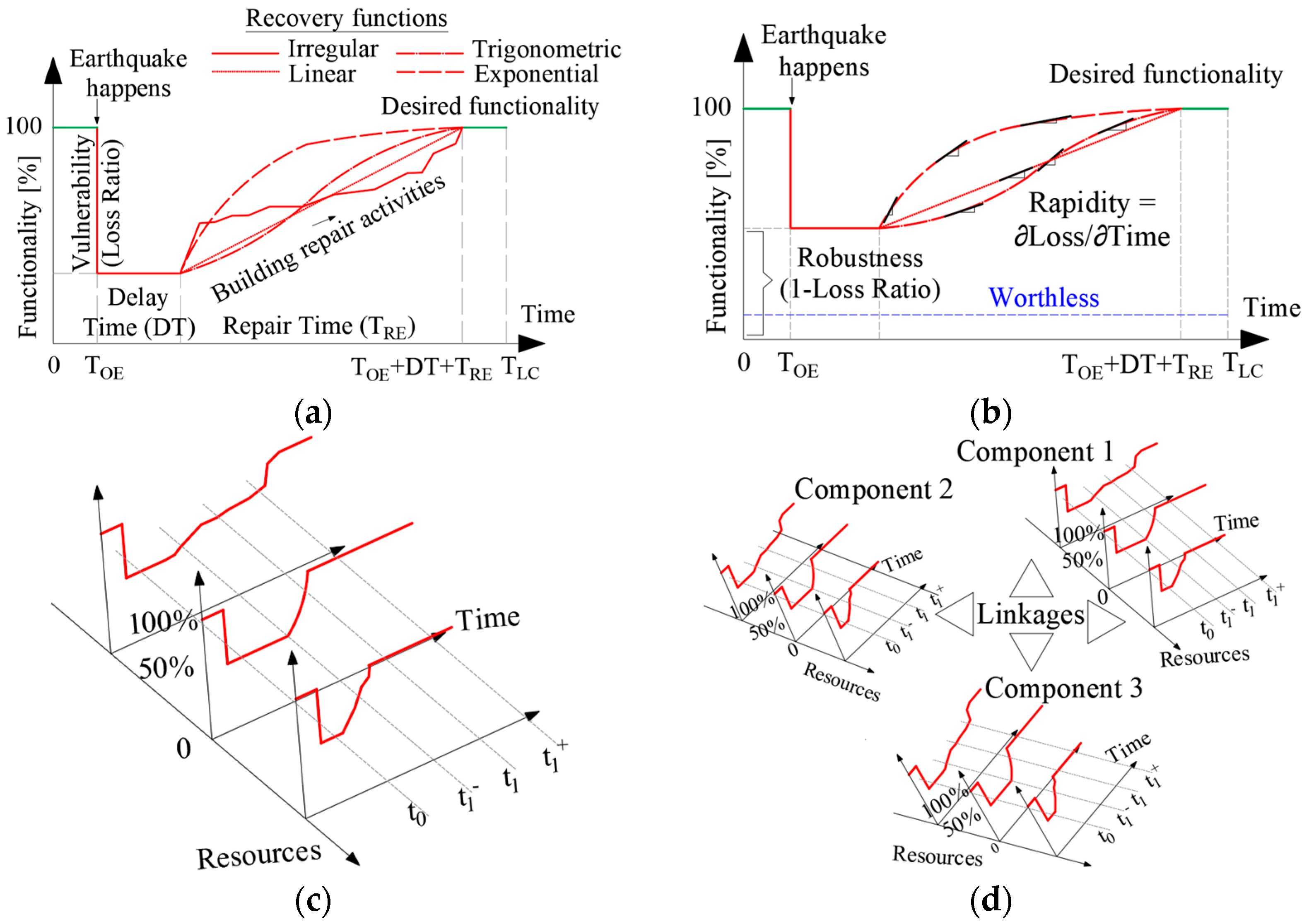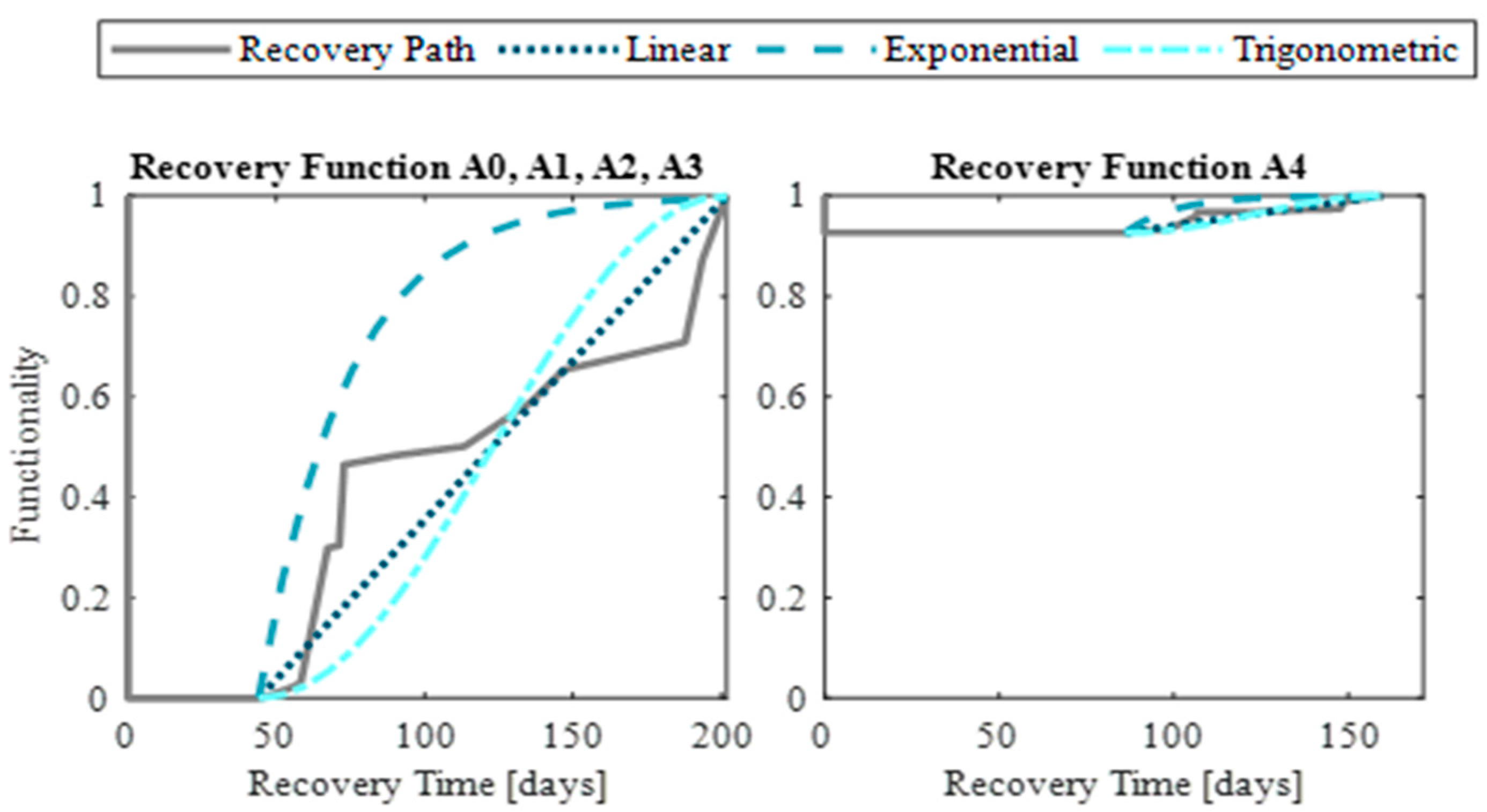Figure 1a illustrates the general concept of a recovery function. Initially, the system, which can be an individual building or a community, is operating normally (i.e., 100% functionality or normal operation activities) until it is disturbed by a seismic event (i.e., earthquake happens at time T0E). The functionality of a building then drops to a certain amount—this portion is associated with the seismic vulnerability, which depends on the earthquake intensity and seismic performance of the structural and nonstructural elements. 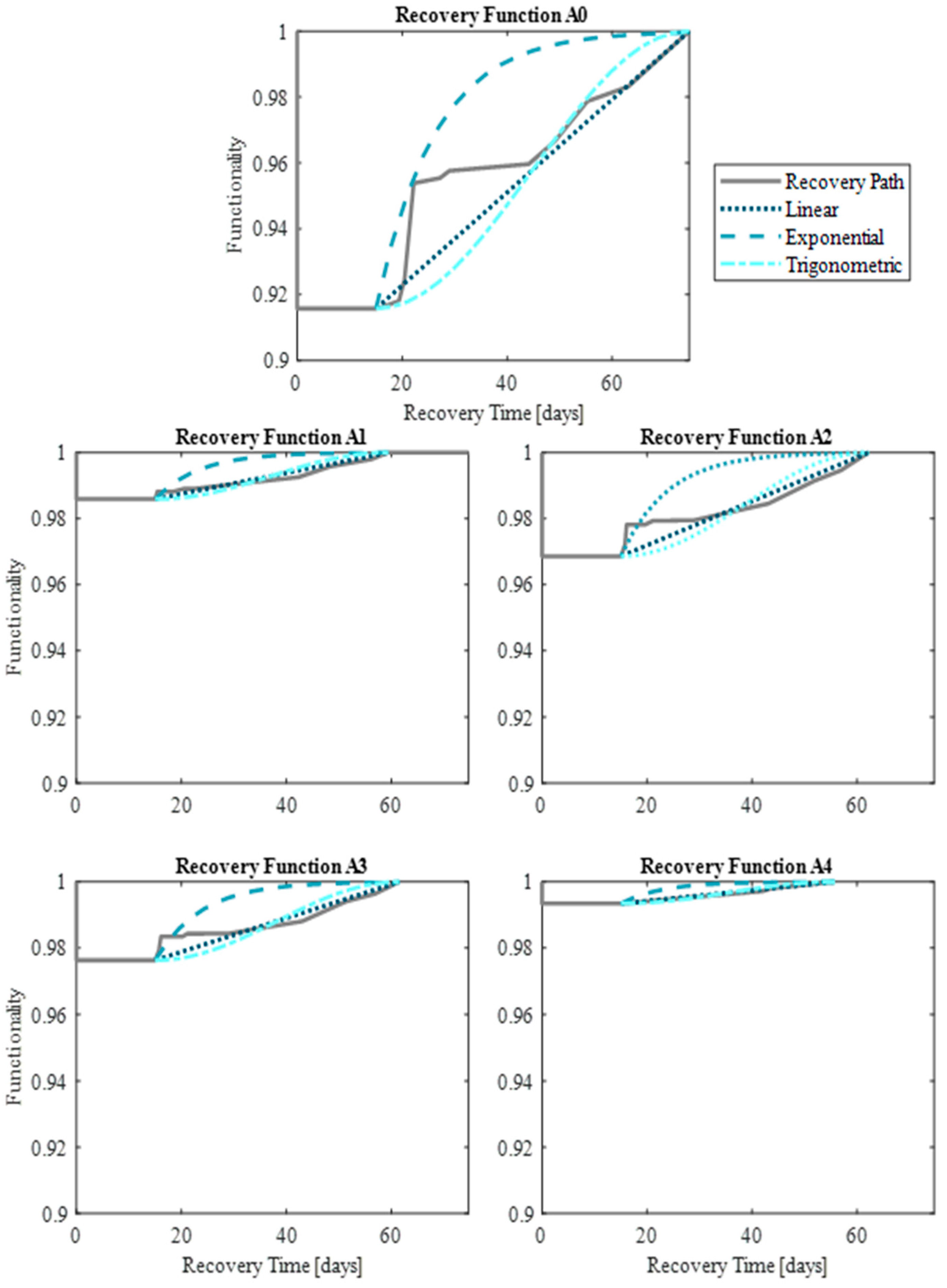This seismic vulnerability is expressed as the loss ratio caused by that seismic event [10]. The horizontal axis represents the recovery time of the building, where any time after T0E indicates the period in which the building is unable to fully operate (i.e., downtime). Once the functionality of a building drops, there is a period in which it remains constant, while the building does not regain any functionality. This period refers to the delay time (DT), which accounts for all external activities that need to be carried out before repairs in the building begin. This includes structural inspections, permits, financing to utility restoration (i.e., lifelines, such as electricity, water, road, and any other external components that enable the building to restore normal operations). The components of the delay are further detailed and explored in the subsequent subsections. Once the delays have been estimated, the repair process begins, i.e., repair time (TRE). The recovery path will likely have an irregular shape, but it can be idealized by different recovery functions, as illustrated in Figure 1a, such as linear [10], exponential [40], or trigonometric [41]. The expressions in Equation (1) mathematically describe these three functions.

$$\mathrm{funcionality} \mathrm{functions}\{\begin{array}{c}\mathrm{linear}:{\mathrm{f}}_{\mathrm{rec}}=\left(1-\frac{\mathrm{t}-{\mathrm{t}}_{0\mathrm{E}}}{{\mathrm{T}}_{\mathrm{RE}}}\right) \\ \mathrm{exponential}: {\mathrm{f}}_{\mathrm{rec}}=\exp \left(-\left(\mathrm{t}-{\mathrm{t}}_{0\mathrm{E}}\right)\left(\ln 200\right)/{\mathrm{T}}_{\mathrm{RE}}\right)\\ \mathrm{trigonometric}: {\mathrm{f}}_{\mathrm{rec}}=0.5\left(1+\cos \left(\mathsf{\pi }(\mathrm{t}-{\mathrm{t}}_{0\mathrm{E}}\right)/{\mathrm{T}}_{\mathrm{RE}})\right)\end{array}$$

(1)

Resilience can be evaluated during an observation period or the life cycle of the building (TLC), meaning that the system would be evaluated for all seismic events that affect the building’s functionality for which different recovery processes and actions would be foreseen. Furthermore, according to Bruneau et al. [11] and Cimellaro et al. [10], resilience has four main properties, known as 4R—robustness, redundancy, resourcefulness, and rapidity—which are defined as follows:

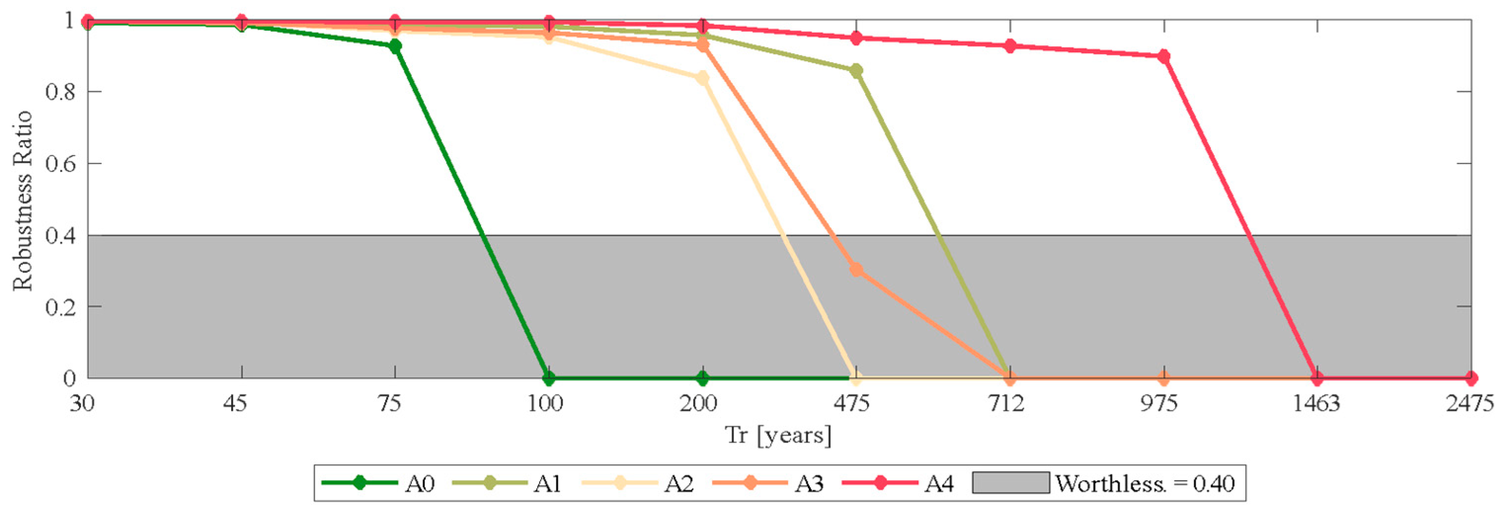
• Robustness: refers to any measure of analysis (e.g., strength and losses) to withstand a given level of stress or demand, without suffering degradation or loss of function. It is evaluated as the residual functionality level following an extreme event, represented in Figure 1b by one minus the loss ratio [10]. Figure 1b also displays a worthless limit, implying that it is impractical to conduct any repair action in a building with robustness under this threshold since it refers to partial collapse or irreparable damage;
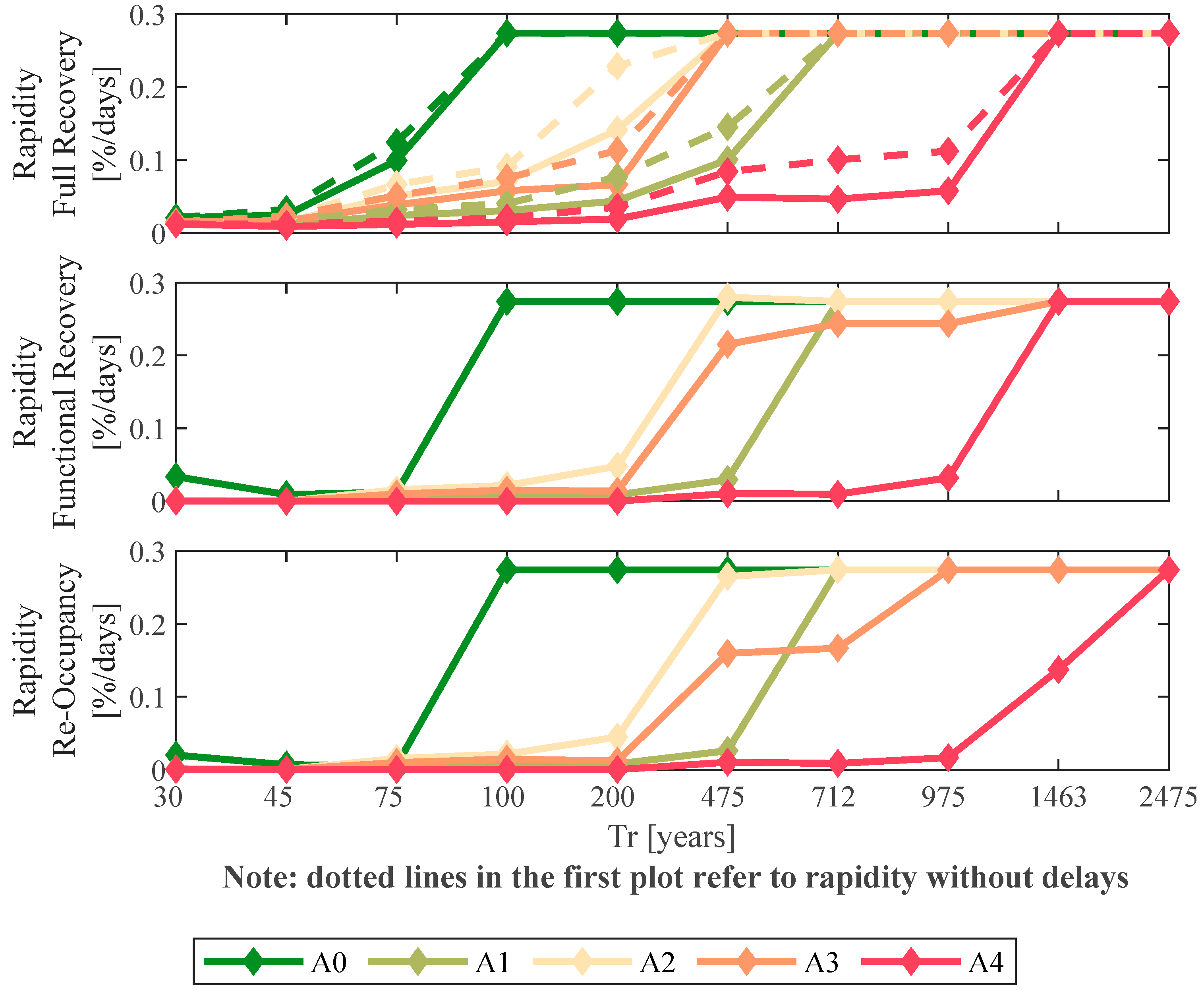
• Rapidity: relates to meeting priorities and achieving goals promptly to contain losses, recover functionality, and avoid future disruption. In Figure 1b, rapidity is represented as the slope of the functionality curve, mathematically expressed as the derivative of the loss function with respect to time. As such, rapidity varies according to the shape of the recovery function. For instance, the rapidity is constant in the case of linear recovery function; on the other hand, an exponential function presents a greater rapidity (faster recovery actions) at the beginning, while it decelerates at the end of the recovery path. Conversely, a trigonometric function presents a lower rapidity (lower recovery rate) at the beginning with respect to the linear one, but then it increases and surpasses the rate of the linear function. Therefore, for the sake of simplicity, an average estimation of rapidity is defined by knowing the total losses and the total recovery time to reach 100% functionality (expressed in percentage/time) regardless of the type of recovery function [10]. However, rapidity does not include the delay time, which considerably affects the rate of recovery in a building;
• Resourcefulness: is the capacity to apply material (i.e., monetary, physical, technological, and informational) and human resources in the process of recovery to meet established priorities and achieve goals [10]. It is, therefore, primarily an ad hoc action, which requires momentary decisions to engage additional and alternative resources [11]. Its quantification is better illustrated graphically in Figure 1c, where the third axis illustrates that added resources can be used to reduce time to recovery. In theory, if infinite resources were available, the time to recovery would asymptotically approach zero, but practically, even in the presence of enormous financial and labor capabilities, human limitations will dictate a practical minimum time to recovery [10].
• Redundancy: is the extent to which measures are replaceable and capable of satisfying functional requirements in the event of disruption, degradation, or loss of functionality [10]. Figure 1d presents the resilience of all components of a system. However, it is important to note that buildings depend on lifelines (e.g., highway and street networks, bridges, electrical systems, piping systems, etc.), meaning that if these are not operative, the building will not be functional, even if all repairs have been concluded. It can be assumed that the performance of a network of elements can be established by a simple aggregation of the performance of individual elements [11]. Moreover, for the case of school buildings and other learning facilities, redundancy can be considered as excess space and classrooms available in the building.

Robustness and rapidity are essentially the desired ends that are accomplished through resilience-enhancing measures and are the outcomes that more deeply affect decisions by stakeholders [10]. On the other hand, redundancy and resourcefulness are measures that define how resilience can be increased, e.g., by adding redundant elements to a system or concentrating damage in replaceable components. All the elements of resilience are important, but robustness and rapidity are seen as the key elements for resilience [11]. In contrast, resourcefulness and redundancy are strongly coupled, but difficult or more complex to quantify [10], as they depend on human factors and available resources; therefore, an analytical function is not provided for these two quantities at this stage. However, changes in resourcefulness and redundancy affect the shape and the slope of the recovery curve, the repair time (TRE), and the robustness. Moreover, resilience is also correlated with four dimensions known as TOSE (i.e., technical, organization, social, and economic) [11]. However, the analysis and review of these four dimensions is beyond the scope of this study.

2.1. Assessment Methodologies

As described, the most common approach to estimate resilience is through a functionality curve that represents the recovery process of a system. However, there are other methodologies and studies that evaluate resilience from different perspectives and parameters. The methods presented in this subsection have been grouped according to similar frameworks, resulting in three groups, detailed as follows:

2.1.1. Index-Based Methods

As mentioned previously, the functionality is estimated from a mathematical function. The complexity of each model is specific to the problem at hand, where different recovery functions may not be able to capture the actual recovery path, but at least are used to approximate it. Many assumptions and interpretations must be made in the quantification of the seismic resilience when diverse factors or fields are considered (e.g., engineering, economics, operations, etc.) into a unique parameter, leading to results that are unbiased by uninformed intuition or preconceived notions of risk. 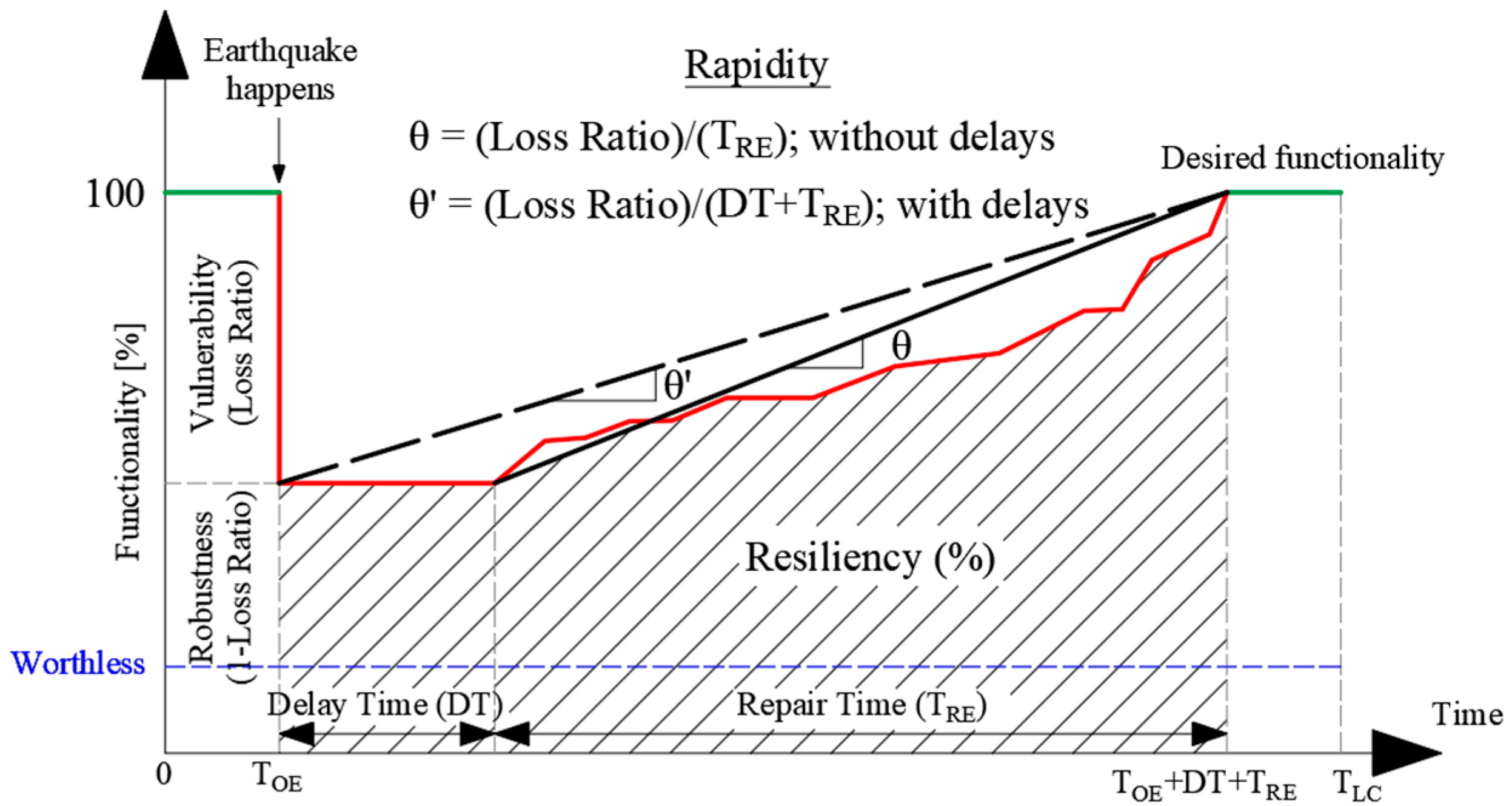For example, Figure 2 illustrates how the area under the recovery function is used as a resilience index [10].

The commonly employed resilience index is defined in a simplified manner as the percentage rate between two functionality areas. The first one corresponds to the area under the curve of the recovery function, which is integrated from the earthquake occurrence to the end of the repairs (when the building has restored its normal conditions). The second area corresponds to the rectangle measured within the same limits, with a height corresponding to full functionality (total replacement cost of a building) and a length of the total recovery time. If the expected losses are considered as a loss ratio (full functionality equals one), the former area is simply normalized by the examination period.

Carofilis et al. [42] examined a seismic resilience-based assessment method applied to school buildings with different retrofitting options. The method was based on Cimellaro et al. [10], assuming a linear recovery function but without considering the delay time. The seismic resilience was estimated using Equation (2), and, as Cimellaro et al. [10] did not consider any type of delays, t₁ was set as the T0E (moment when the earthquake happens), and t₂ was taken as the repair time TRE. However, the integration limits can be modified to include delays or even integrate the recovery function with respect to an observation period (TLC), which considers resilience with respect to the life cycle of a building. This means that if a delay time is considered, t₂ is defined as DT + TRE if T0E is set as zero. This equation has also been used by other authors in resilience assessment studies (Anwar and Dong [9]).

$$Resilience [\%]={{\displaystyle \int }}_{t_1}^{t_2}\left(\frac{f_{rec}\left(t\right)}{t_2-t_1}\right)dt$$

(2)

The seismic resilience index is used to evaluate both hypothetical and real cases. For example, this evaluation parameter was used to assess Iranian school buildings, including post-recovery and retrofitting processes [43]. Immediately after the occurrence of the 2017 Ezgeleh earthquake and in the following three years, the recovery process of the school buildings was monitored, and the gathered information was used to extract the seismic resilience indices. School buildings that had been retrofitted before the 2017 Ezgeleh earthquake demonstrated a high level of resilience with full functionality. Moreover, those schools that had not been retrofitted before the earthquake had the lowest resilience indices with zero robustness [43]. Similarly, the seismic resilience of another Iranian school building was evaluated with four hazard levels, namely, 50%, 20%, 10%, and 2% probability of exceedance in 50 years [44]. The results indicated that moment-resisting frames retrofitted with base isolation have a higher resilience index and lower repair costs compared to the conventional fixed-base system. Conventional engineering judgement suggests that if the structural damage exceeds 35% of a building reconstruction cost [44], retrofitting is no longer a feasible repair alternative, and the structure should be reconstructed immediately. Moreover, it is also assumed that if the school’s functionality decreases by more than 50%, the school must be evacuated until the retrofitting operations are completed, meaning that the utilization process does not take place before the retrofitting operations are completed [44]. Similar criteria were used by O’Reilly and Sullivan [45] to evaluate the seismic vulnerability of Italian school buildings, assuming that when the expected economic losses exceed 60% of the replacement cost of the building, the stakeholder would decide to demolish rather than repair the existing building. On the other hand, Elwood et al. [46] reported a much lower ratio following the Canterbury earthquakes of 2011 and 2012 in New Zealand, noting that over 50% of the structures presented a damage ratio ranging from 2 to 10% were demolished. This peculiar threshold is a result of a severe legislative decision that penalized old RC buildings by labeling them as seismically vulnerable regardless of their real damage condition. In this study, for the Italian context, the demolition threshold of 0.6 adopted by O’Reilly et al. [20] was used to estimate robustness through Equation (3), thereby leading to the robustness threshold of 0.4 (1–0.6). This means that for an expected loss ratio equal or higher than 60% of the total replacement cost of a building, or for a robustness lower or equal to 40%, it is more practical to demolish the structure rather than spending resources to restore its original configuration/use.

$$Robustness=1-Loss ratio$$

(3)

Rapidity, in turn, is modified to account for the delays. As observed in Figure 2, if delays are considerably long, the rapidity of the system decreases (θ’). Conversely, if delays are short, the rapidity of the system increases (θ). In this study, Equation (4) is proposed to compute rapidity, whether accounting for the delay time or not (i.e., T corresponds to the recovery time that may or may not include delays).

$$Rapidity, \theta \left[\%/Time\right]=\frac{Loss ratio}{T}\times 100\%$$

(4)

It is clear that the seismic resilience of buildings is estimated by different metrics. For example, the assessment is based solely on the four main components of resilience: rapidity, robustness, redundancy, and resourcefulness of which only the first two are numerically quantified. Even though redundancy and resourcefulness influence rapidity and robustness, they cannot be numerically quantified and depend on monetary or human resources. Given that redundancy and resourcefulness cannot be estimated analytically, these two dimensions of resilience are not evaluated in this study.

2.1.2. Methods Based on Recovery States

The approaches within this group address postearthquake functionality and recovery states, including a sequence of damage states that a building undergoes before regaining normal operation activities. The Resilience-based Earthquake Design Initiative (REDi) Rating System developed by Almufti and Willford [1] provides to owners and other stakeholders a framework for implementing resilience-based earthquake design according to the PEER PBEE methodology [47]. It is a holistic beyond-code design method that integrates planning and assessment for achieving a much higher performance [1]. The REDi framework assigns a building a rating class from its three-tiered system (i.e., Platinum, Gold, or Silver). To assign a rating class, it is necessary to satisfy mandatory criteria of the baseline resilience objectives defined in the REDi guidelines [1]. Even though the method considers only the design earthquake level, the framework can be implemented for other demand levels or performance states. Given their usefulness, the REDi guidelines are used in this study to determine the recovery states and their features (e.g., delay time, repair time, element repair states, functionality level, etc.) for the seismic resilience assessment of existing buildings, when no rating classes are evaluated and assigned.

REDi is a practical framework to estimate influential aspects, such as long lead-time, delays due to utility downtimes and impeding factors, to result in three possible recovery states:

• Reoccupancy. A building is safe enough to be occupied (e.g., as a shelter). If damage is apparent, this typically requires an inspection. Any damage to structural and nonstructural components is minor and does not pose a threat to life safety.
• Functional Recovery. Condition to regain the facility’s primary function. This would require restoring power, water, fire sprinklers, lighting, and HVAC systems, while also ensuring that elevators return operational. It also indicates the time required for the resumption of specific functions particular to a certain occupancy type. Examples include emergency services and typical services in hospitals or classes in educational facilities.
• Full Recovery. Repairs are required primarily for aesthetic purposes (such as painting cracked partitions) to restore the building to its original pre-earthquake condition.

All of these recovery states depend on an average damage state reported for each building element after conducting a loss assessment (PACT [48]). The REDi guidelines provide average repair classes for most structural and nonstructural components based on their average damage state. These repair classes (1, 2, and 3) are related to the recovery states. For instance, components in repair class 1 are expected to experience minimal or minor cosmetic damage. An element in repair class 2 has a certain level of damage that does not pose a life safety risk. Finally, an element in repair class 3 has a heavily damaged component that represents a life safety risk or it is not operative. To achieve a certain recovery state, the components influencing that state must be repaired. The reoccupancy recovery state requires the repair of components in repair class 3 only. Similarly, the functional recovery state requires the repair of the elements in repair classes 2 and 3. For full recovery, all elements must be repaired.

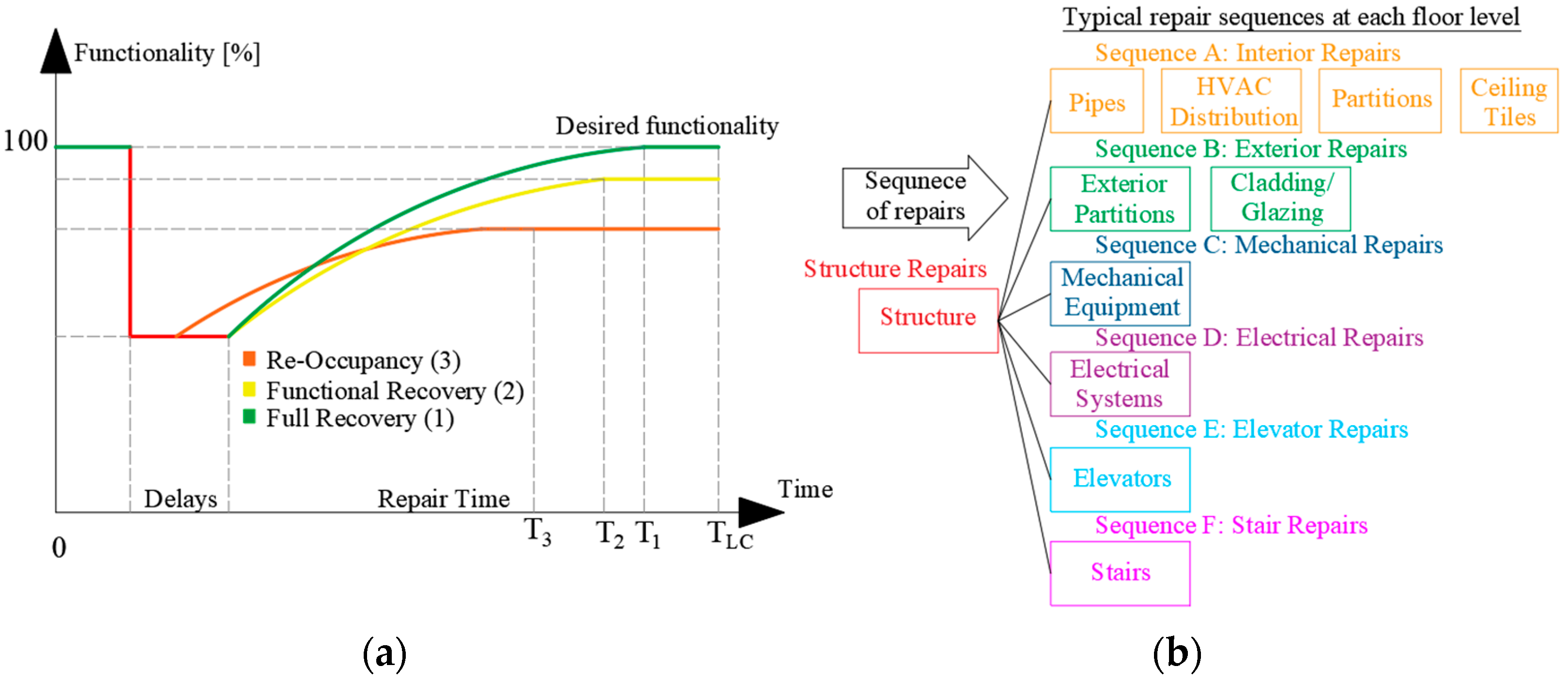
Figure 3a exemplifies the recovery paths for the three aforementioned recovery states. For reoccupancy, the building regains a certain level of functionality after the seismic event; the recovery time needed to reach such states is much less than that of the other two states. Additionally, the delays are shorter since the building does not require that all services are operative and reoccupied. The functional recovery has a much higher functionality and thereby a longer recovery time. Finally, the full recovery state represents the conditions where the building has regained normal operation activities. Furthermore, Figure 3b displays the sequence of repairs followed by each recovery state depending on the damage reported by each repair group (Tables 4 and 5 of the REDi guidelines [1]). The sequence starts with the structural repairs that must be completed before proceeding with any other repair component. These repair groups (e.g., interior repairs, exterior repairs, and mechanical repairs) can be addressed in parallel as long as the maximum number of workers is not exceeded [1].

The delays between the earthquake event and the initiation of repairs, which are significant, are referred to as impeding factors and include the time it takes to complete postearthquake building inspections, secure financing for repairs, mobilize engineering services, obtain permitting, mobilize a contractor and necessary equipment, and for the contractor to order and receive the required components including long lead-time items [1]. The utility disruption is another component of the delay times, which is likely to occur for a design-level earthquake and must be considered for buildings attaining a full recovery state, including lifelines, such as electricity, gas, and water lines.

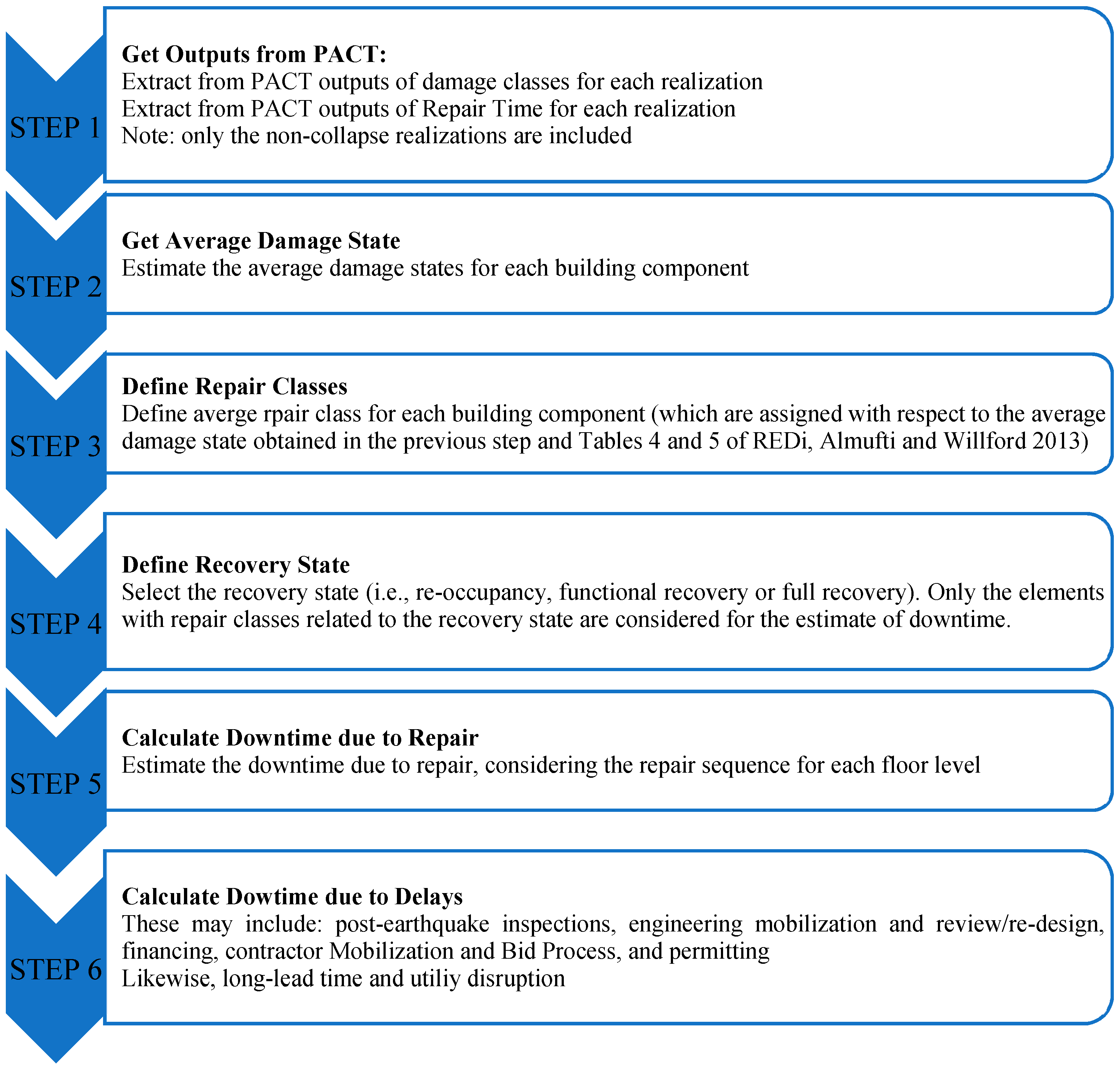
The REDi framework is also very practical for a good estimate of the downtime, which is determined in a more rigorous fashion from a loss assessment using the software PACT [48]. Despite acknowledging the US-specific limitations of this software for conducting a loss assessment in regions outside of the US, the outputs that this tool generates can be used to carry out a comparison among strategies. 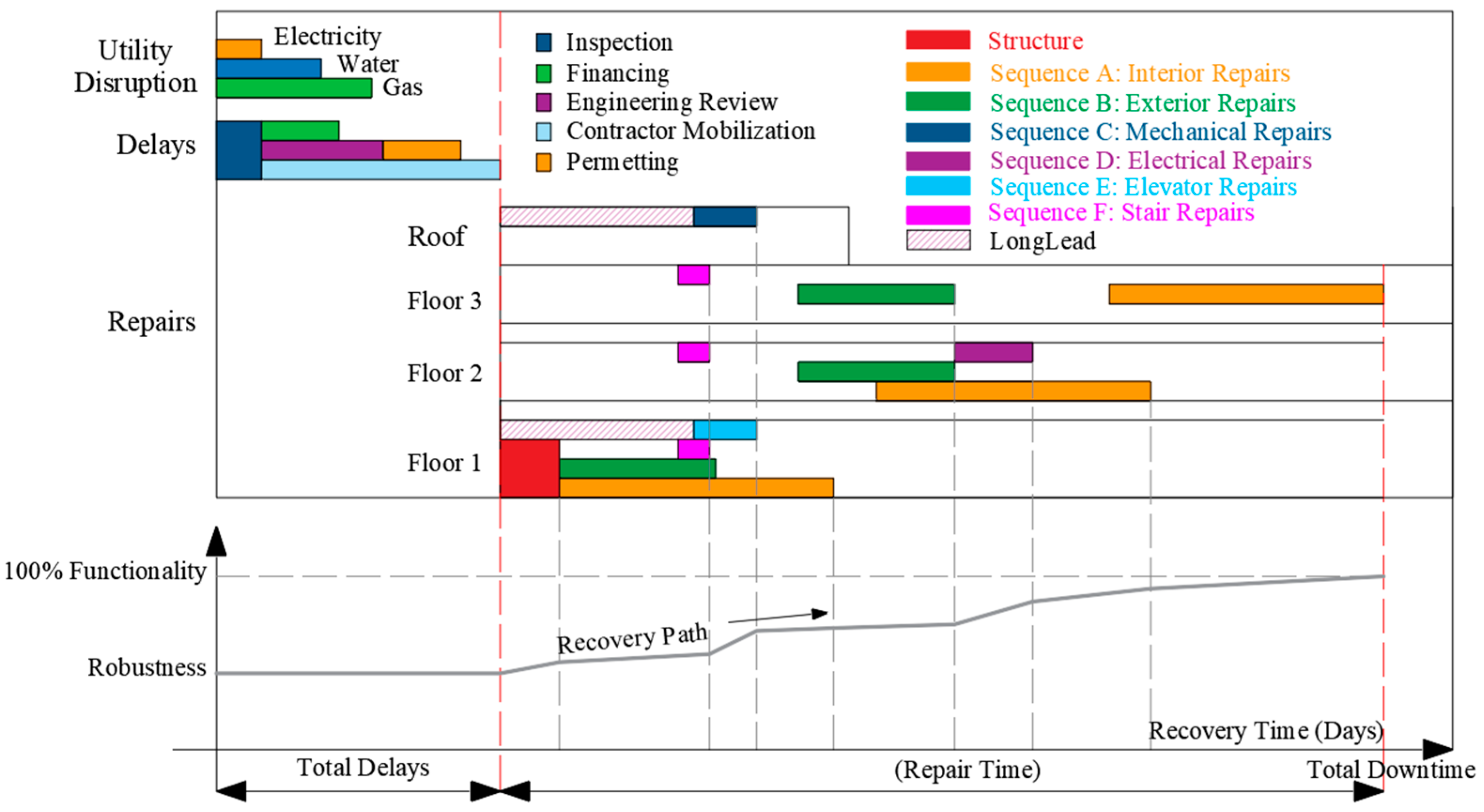Figure 4 lists the steps involved to obtain the recovery time. The recovery time framework for the reoccupancy state includes impeding factors and any building components classified as repair class 3. On the other hand, the recovery time framework for functional recovery integrates utilities and impeding factors as delays, and then all components defined as repair classes 2 and 3 are considered. Similarly, the downtime framework for full recovery includes utilities and impeding factors and considers all repair classes (i.e., 1, 2, and 3). The sequence of delays due to impeding factors is initiated by the postearthquake inspections, followed by the financing, engineering mobilization and review, and contractor mobilization. Contractor mobilization leads to permitting and any long lead-time components.

Furthermore, Figure 5 illustrates the repair sequence to reach full recovery for a four-story building. REDi presents a reasonable sequence to conduct repairs; therefore this repair schedule is used to estimate the recovery function or path as displayed at the bottom of Figure 5. The recovery path is determined by adding the cost associated with each repair sequence (regaining of functionality) and by adding the total delays with the time associated with each repair sequence (total downtime). It is also important to notice the availability of financial resources, which, when lacking, considerably lengthen the time due to delays. In that case, other sources of financing, such as credits or loans, need to be explored. Eghbali et al. [43] revealed that the most noticeable factors causing delays to the start of the renovation of Iranian school buildings after the 2017 Ezgeleh earthquake were lack of sufficient funding by the government and/or donors, time-consuming procedures for the selection of contractors, use of school buildings as temporary shelters for local residents, and delays in the removal of school equipment by the Ministry of Education. Similarly, the time representing the long lead is followed after the contractor mobilization, indicating that if financing exceeds contractor mobilization, one does not have to wait until the repair tasks begin to consider the long lead. As such, the repair of components depending on long lead will not delay the repair activities.

Overall, the REDi guidelines provide a comprehensive framework to evaluate different resilience parameters. Even though the framework is challenging and time-consuming, due to the level of analysis to carry out and subsequent postprocessing of outputs, it yields relevant aspects, such as delays, total downtime, repair classes, and resilience category, among others, that can evaluate seismic resilience in a more precise way. However, one may argue that, given the context in which the REDi guidelines were developed, they should be applied only to case studies in the United States. While it is evident that the resilience measures are not fully representative of the region where the assessment is conducted, for comparative purposes, the framework can be still used as illustrated in subsequent sections through the comparative analysis of retrofitting solutions, including resilience as an evaluation parameter.

2.1.3. Performance-Based Multicriteria-Based Methods

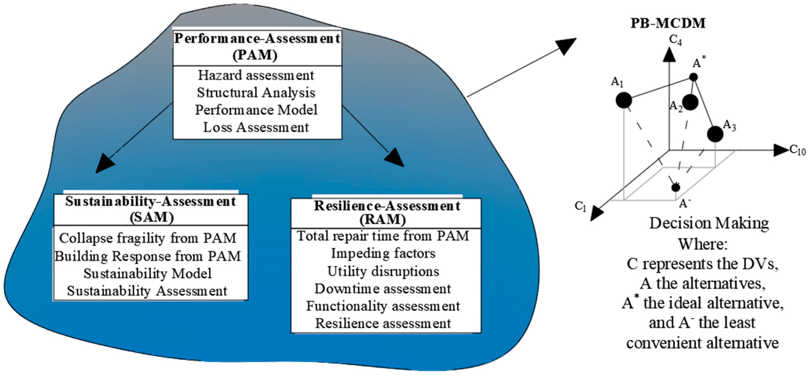
Anwar et al. [49] introduced a performance-based multicriteria decision-making (PB–MCDM) approach to assess the seismic resilience of buildings from a long-term perspective. The PB–MCDM integrates the performance assessment with the MCDM framework [26], and the seismic resilience is evaluated for a range of intensities and includes several consequences (i.e., economic, social, and environmental consequences) [49]. Therefore, to implement the PB–MCDM, three types of analyses need to be carried out: (1) performance assessment module—PAM (loss assessment), (2) sustainability assessment module—SAM (expected consequences: social and environmental), and (3) resilience assessment module—RAM. These three metrics are then integrated into an annualized value, and through an MCDM analysis, the most convenient retrofitting option is selected (Figure 6). This section is divided by subheadings. It provides a concise and precise description of the experimental results, their interpretation, and the experimental conclusions that are drawn.

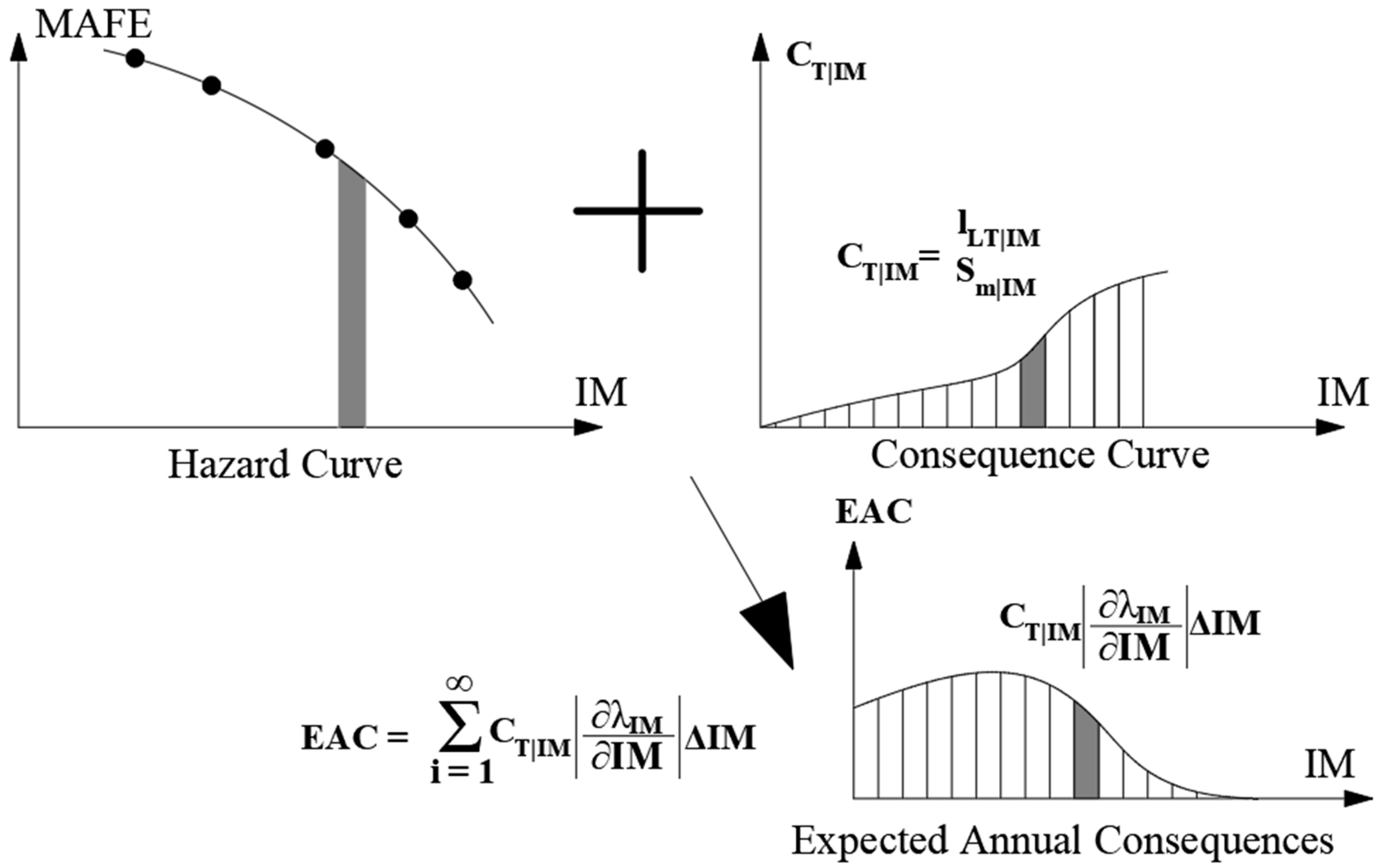
At a first glance, the PB–MCDM framework appears as an extensive methodology (i.e., four modules have to be evaluated); however, the method is simplified by using the software PACT [48], from which the three first modules (PAM, SAM, and RAM) can be quickly obtained. Each module is evaluated for different intensities, and then all the PAM, SAM, and RAM parameters are integrated into a single metric. The integration procedure, illustrated in Figure 7, combines the mean annual frequency of occurrence and the total consequence curves, considering hazard scenarios converted to expected annual consequences (EACs). Finally, the MCDM [26] is applied to the parameters obtained from these modules.

Anwar et al. [49] evaluated three different earthquake intensities: FLE (Frequent-Level Earthquake), DLE (Design-Level Earthquake), and MCE (Maximum Considered Earthquake) when analyzing a 4-story RC building with three retrofitting alternatives. Five parameters were considered for the MCDM evaluation: seismic loss (economic losses), sustainability, through three parameters (casualties, equivalent carbon emissions, and embodied energy), and resilience. The repair time, sequence of repairs, and total repair time were determined using the REDi methodology [1]. The alternative with the highest relative closeness [26] was considered as the best retrofit option among the considered alternatives.

Furthermore, Anwar et al. [49] found that long-term consequences result in different closeness coefficients, and thereby long-term consequences greatly influence the rank preference. As such, the expected long-term economic losses and environmental consequences (embodied carbon emissions and embodied energy) are also contemplated in this study and determined through Equations (5) and (6), respectively:

$$E\left[l_{\left(LT\right)L_{T|tmax}}\right]=\frac{L\lambda }{r}(1-e^{-rtmax})$$

(5)

$$E\left[S_{(LT)L_{T|tmax}}\right]=S\lambda tmax$$

(6)

where L accounts for the expected economic losses for a given intensity; λ is the frequency of the earthquake for a given intensity determined from a hazard curve; r is the financial discount rate; tmax is the investigated period; S is a parameter that represents an environmental consequence (i.e., embodied carbon emissions or embodied energy).

The PB–MCDM adopted by Anwar et al. [49] focuses on sustainability and resilience aspects. However, the versatility of the MCDM allows it to incorporate many additional aspects, such as social, technical, and environmental ones. For a more comprehensive evaluation, PB–MCDM should incorporate other important variables, such as cost, duration of work, architectural impacts, etc., which have been demonstrated to control and alter the selection of the most favorable strategy (Carofilis et al. [42]).

Table 1. Main advantages and shortcomings of the reviewed methodologies.

Seismic Resilience Approach	Advantage	Disadvantage
Index-based Methods	Simple and easy to quantify a resilience parameter (area under the curve of recovery function). Two of the main properties of resilience are evaluated (i.e., rapidity and robustness)	Delays are not considered, if any delay is assumed, then rapidity decreases. A structure that has lost its functionality completely is granted a resiliency of 50% and not 0.
Methods Based on Recovery States	Addresses delays. Useful to represent the recovery process/repair activities. Considers three different functional recovery states.	Requires a detailed loss estimation analysis (e.g., using PACT). Recovery time outputs from PACT need post-processing to adjust them to the framework. Some assumptions refer to the U.S. context (only applicable in that region).
Performance-based Multicriteria-based Methods	Integrates several evaluation parameters. Resilience is evaluated for different intensity levels. Uses the expected annual consequences as a metric for the decision variables.	MCDM is influenced by the weight vector, which is affected by importance given to the variables. Requires specialized software (e.g., PACT).

summarizes the main features of the reviewed methodologies highlighting the main advantages and disadvantages for each approach.

3. Application and Comparison of the Available Assessment Methodologies

3.1. Case Study Building

An RC moment-resisting frame (MRF) school building (illustrated in Figure 8), located in Isola del Gran Sasso d’Italia, Abruzzo, Italy, with unreinforced masonry (URM) infills was adopted as a case study building. It has two above-ground stories and a small partial basement at the east end. The first and second floors have an area of approximately 630 m² and interstory heights of 3.75 m and 4.25 m, respectively. The building is a typical Italian construction dating back prior to the introduction of modern seismic design provisions (Prota et al. [50]). A more detailed description of the building, along with architectural plans and elevations, is found in Prota et al. [50], and its detailed seismic performance evaluation is found in Clemett et al. [30]. Four seismic retrofit schemes were evaluated: A1—local strengthening with carbon FRP (CFRP); A2—global strengthening with concentric steel bracing-system; A3—CFRP strengthening combined with concentric steel bracing-system, and A4—CFRP strengthening combined with viscous dampers. These retrofitting strategies were initially conceived to improve the building’s structural capacity and comply with code-defined limit state requirements of NTC 2018 [17]. However, when these criteria cannot be met, due to excessive cost or material requirements, the maximum improvement that can be implemented is accepted and adopted. Additionally, all the retrofit configurations present URM infills detached from the RC frame through the introduction of a seismic gap to eliminate column–infill interaction and reduce the shear forces acting on the columns. The design procedure for each of the retrofit alternatives and all the associated assumptions are found in previous studies (Carofilis et al. [42]; Clemett et al. [51], and Clemett et al. [30]).

3.2. Characterization of Seismic Hazard Site

The case study building is located in Isola del Gran Sasso d’Italia, a region characterized by medium–high seismicity (De Risi et al. [13] and Stewart et al. [14]). To evaluate the nonlinear dynamic seismic response of the building, a multiple-stripe analysis (MSA) [52,53] was performed. The software OpenQuake (GEM 2019 [54]) was used to carry out the probabilistic seismic hazard analysis (PSHA) and disaggregation analyses for ten return periods: 30, 45, 75, 100, 200, 475, 712, 975, 1463, and 2475 years (defined by NTC 2018 [17] for a building type III). A set of 20 ground motion records in both orthogonal directions were selected for each. The average spectral acceleration (AvgSA, Eads et al. [55], and Korangi et al. [56]) illustrated in Figure 9 for each return period was used as the intensity measure (IM) to determine all the demand parameters. Adopting AvgSA as the IM represents an advantage, given that the same records can be used for the entire set of retrofitting alternatives, corresponding to different fundamental periods. As explored by O’Reilly [56], the AvgSA is a more suitable IM for intensity-based analyses (e.g., fragilities functions) due to its moderately low level of dispersion across a range of assessed intensities. Other IMs such as conditioned spectral acceleration may lead to a potential bias unlike AvgSA. The record match was done for a period range of 0.2 Tgm–1.5 Tgm, where Tgm is the geometric period established as the square root of the product between the two fundamental periods for each model. Further details about the ground motion selection are found in Carofilis et al. [42]. Figure 9 also includes the acceleration response spectrum for the return period of 712 years, illustrating how the AvgSA is obtained through the range of periods (Tmin to Tmax).

3.3. Preliminary Seismic Resilience Evaluation

Firstly, two of the main properties of resilience, namely, robustness and rapidity, were evaluated for the school building (A0) and its four retrofitting configurations (A1 to A4), using Equations (3) and (4), respectively. Figure 10 illustrates the robustness for all assessed models, which were obtained as the median of the set of 20 ground motion records for each return period. The worthless limit was set as 0.4 (represented by the grey area), as explained in Section 2.1.1, meaning that cases below this limit suffer from severe damage leading to demolition. The as-built school building presents a premature loss of robustness for return periods longer than 100 years. This premature degradation is represented by the points that fall on the worthless area, meaning that the school building has collapsed or that irreparable damage has occurred. On the other hand, it is clear that all retrofitting strategies increase the robustness of the original configuration, with A4 being the strategy that attains the most substantial improvement and A2 the one with the least increase. The retrofitting strategies are ranked according to the level of robustness enhancement (i.e., highest to lowest) as: A4–A1–A3–A2.

In the case of the average rapidity (Equation (4)), three recovery states (i.e., reoccupancy, functional recovery, and full recovery) are featured in Figure 11. In most of the reviewed studies, rapidity is taken as the ratio between the expected losses and the recovery time and measures the rate at which the repairs are conducted. Nevertheless, if rapidity is considered as a measure of resilience, it needs to account for the delays that greatly impact the downtime, lengthening it. Therefore, a rapidity evaluation can be split in two scenarios: one focusing only on the repair activities and another considering it as a metric of resilience, which considers the total downtime. The two rapidity scenarios (with and without delays) and recovery states correspond to the median of the noncollapse cases determined from the 20 ground motion records for each return period. The rapidity with delays (θ’) is compared with rapidity without delays (θ) in the first plot of Figure 11. It is noted that when delays are not considered, the rapidity is greater, especially for return periods longer than 200 years, while for low return periods, rapidity with delays is slightly greater than rapidity without delays. This is explained by the main components of delays. Utility disruption (i.e., lifeline operation) and impeding factors (all activities that need to be carried out before repair begins) are influenced by the earthquake intensity. For more frequent earthquakes, utility disruption and impeding factors are not generated or are low enough so as not to impact the beginning of repairs in a building (i.e., recovery time tends to the repair time). On the other hand, for rare seismic events, these two components are likely generated, and thereby the downtime is lengthened. The downtime was estimated through the REDi guidelines provided in Figure 4. Despite being based on data for the United States and the fact that the Italian context has different seismicity, currency, and building typologies, some of the assumptions available in REDi were adopted in this study for the sole purpose of comparison of different alternatives. While this does not accurately measure the exact resilience of the school building and retrofitting options, these assumptions still enable a resilience comparison based on the same assumptions to be carried out. Accordingly, a median value of 2 days (essential facility) was adopted for the postearthquake inspection. Engineering mobilization was characterized by assuming engineering contracts of 2 weeks and 4 weeks to conduct any review design for damage states 1 and 3, respectively. Financing was assumed to come from insurance (6 weeks); this is a dominant parameter since in the case of no financial support, obtaining a loan or any type of financial aid can take 48 weeks or more (according to the Small Business Administration SBA-backed loans). In terms of contractor mobilization, 3 weeks and 7 weeks were assumed for damage states 1 and 3, respectively. Finally, for permitting, 1 week and 8 weeks were considered for damage states 1 and 3, respectively.

Moreover, a limit of (1/365 = 0.0027) was set for rapidity and refers to an expected loss ratio of one (i.e., expected loss equal to the total replacement cost of the building) divided by 365 days (a limit time assumed to demolish and rebuild the same school building). For simplification, it was considered that this represents a good estimate of the time needed to demolish and rebuild the case study building. The as-is configuration (A0) reaches the rapidity limit for return periods longer than 100 years. Notably, A0 results in an expected loss ratio of one due to the high collapse vulnerability, meaning that for longer return periods, the school building must be demolished and rebuilt. On the other hand, the best improvement in rapidity is achieved by A4 for a wide range of intensities. Once again, the preference of the retrofitting alternatives according to the improvement of rapidity is as follows: A4–A1–A3–A2. Additionally, the rapidity for the other repair states shows that A1 has a better performance. This retrofitting strategy does not considerably change the seismic demand parameters, such as peak floor acceleration (PFA) and peak story drift (PSD), which tend to be identical to the A0 ones. A1, however, increases the capacity of the structural elements, and thereby less structural damage is reported. When less damage is generated, the time required to repair a component is less. More importantly, for the reoccupancy recovery state, only components in repair class 3 need to be repaired. Consequently, the rapidity for A1 is improved since both the losses and the repair time decrease. The same occurs for the functional recovery state where components with a repair class higher than 2 need to be considered.

3.4. Seismic Resilience Index

Concerning the seismic resilience index, four recovery paths were explored, as illustrated in Figure 12 for a return period of 712 years (i.e., intensity associated with the life safety limit state for the case study building). The linear, exponential, and trigonometric shapes are described in Section 2, whereas the irregular shape (grey line labeled as recovery path in Figure 12), which represents an estimate of the recovery time based on the results of the detailed damage analysis, was calculated by adding the repair cost sequence and repair groups as illustrated in Figure 5 and described in Section 2.1.2. A comparison among all recovery functions illustrated in Figure 12 was sought, as several studies have idealized the recovery process with only one of the three aforementioned recovery functions. For some models, the linear and trigonometric functions seem to better approximate the recovery path. For the life safety limit state (SLV) [17], A4 is the only strategy that does not completely lose its robustness, which is still above 90%. For the remaining models, the recovery process starts from zero, meaning that these building configurations have been demolished and rebuilt completely.

Similarly, Figure 13 illustrates the recovery functions for a return period of 75 years (damage control limit state, SLD [17]). For this limit state, it is expected that the building regains full functionality promptly. All the models lost just a small fraction of their robustness. However, the downtime for most retrofitting strategies extends up to 60 days. The delays for this earthquake scenario are related to inspection, engineering mobilization, and financing to repair the components that have been damaged. Nevertheless, as the robustness remains above 90%, after the earthquake, the building is under a functionality recovery state meaning that some portions of the building remain operative.

Even though the recovery functions follow different patterns, once these are integrated through Equation (2), they lead to similar seismic resilience indices, as illustrated in Figure 14 for each return period. The indices from the linear and trigonometric functions turn into identical values, while the exponential function produces the largest index (due to the larger area under the curve). The trigonometric and linear functions present similar values, which are very close to the irregular recovery path, especially for low intensities (i.e., return periods less than 100 years). On the other hand, the exponential function produces much higher values with respect to the other two functions and irregular recovery paths. Indeed, the values seem to be twice the irregular recovery path for return periods longer than 100 years. The linear function is the most common to idealize a recovery path. However, the recovery path is not constant throughout the whole repair process of a building. The repair time and losses depend heavily on the repair groups, which represent different fractions of the total replacement cost of the building, meaning that the repair rates cannot be identical. Consequently, even though the linear recovery function is the simplest way to proceed, the repair path does not represent the different repair rates that are developed throughout the building’s functionality restoration. Additionally, the repair process is influenced by whether some activities are carried out in parallel or not.

It is evident that the irregular recovery process (derived from REDi [1]) is the most appropriate way to proceed when the target is to study the full recovery process. However, when the assessment focuses on the overall seismic resilience index, any of the three idealized functions can be adopted. In terms of comparison, all four recovery paths have the same pattern with strategy A4 standing out as the most seismically resilient configuration followed by A1, A3, and lastly A2.

Finally, the PB–MCDM discussed in Section 2.1.3 was applied for which

Table 2. Decision matrix for PB–MCDM [49], also using long-term consequences.

Model	EA Economic	EA Carbon Emission	EA Embodied Energy	EA Resilience(%)	EA Economic (Long-Term)	EA Carbon Emission (Long-Term)	EA Embodied Parts (Long-Term)
A0	23,894.7	16,291.3	254,393	3.8	8.37 × 103	1.11 × 104	1.75 × 105
A1	5450.1	3375.6	53,806.1	4.4	0.94 × 103	0.89 × 103	1.79 × 104
A2	12,360.6	7243.8	114,172.3	4.2	1.87 × 103	1.80 × 103	3.15 × 104
A3	9510.86	5556	87,765.9	4.3	1.49 × 103	1.41 × 103	2.52 × 104
A4	2811	1635.6	27,122.6	4.4	0.59 × 103	0.63 × 103	1.24 × 104

contains the elements of the decision matrix [26] and

Table 3. Rank preference for the decision matrix of Table 2.

Condition	Rank	Relative Closeness
Without Long-term Consequences	A4–A1–A3–A2–A0	0.95–0.87–0.71–0.59-0.05
With Long-term Consequences	A4–A1–A3–A2–A0	0.96–0.95-0.90–0.87-0.04

the preference ranking. Four evaluation parameters were considered for the MCDM, namely, expected annual economic losses (EA Economic), expected annual carbon emission (EA Carbon Emission), expected annual embodied energy (EA Embodied Energy), and expected annual resilience index (EA Resilience). Equal importance, i.e., a weight of 0.25, was given to all the decision variables (DVs). The expected long-term consequences were estimated through Equations (5) and (6). As the consequences of the PB–MCDM framework are derived from PACT, the A0 building configuration was also included in the MCDM analysis, considered as an alternative where no actions are carried out to improve the seismic resilience of the school building.

The ranks for the two analyses (with and without long-term consequences) are reported in Table 3. For these two cases, the rank preference has similar relative closeness. For this case study building, the long-term consequences seem to not influence the selection of the most convenient alternative. Similarly, A0 has the lowest relative closeness (very close to zero), meaning that not carrying out any action to improve the seismic resilience is not practical at all.

Table 4. Seismic resilience parameters.

Model	EA Robustness	EA Rapidity (%/Days)	EA Resilience (%)	Re SLO (%)	Re SLD (%)	Re SLV (%)	Re SLC (%)	RaFR SLD	RaRe SLD	R1 SLD
A0	0.033	4.4 × 10−5	3.8	99.06	95.5	43.9	43.9	9.07 × 10−5	6.49 × 10−5	0.83
A1	0.043	1.4 × 10−5	4.4	99.6	99.1	43.9	43.9	7.12 × 10−7	7.12 × 10−7	0.92
A2	0.04	2.5 × 10−5	4.2	99.4	98.1	43.9	43.9	1.37 × 10−6	1.37 × 10−6	0.90
A3	0.041	2.1 × 10−5	4.3	99.4	98.6	43.9	43.9	1.27 × 10−6	1.27 × 10−6	0.93
A4	0.044	8.5 × 10−5	4.4	99.7	99.6	94.4	43.9	6.31 × 10−9	6.14 × 10−9	0.94
A1RNS	0.043	1.4 × 10−5	4.4	100	99.9	43.9	43.9	8.90 × 10−4	8.90 × 10−4	0.98
A3RNS	0.041	2.1 × 10−5	4.3	100	99.7	43.9	43.9	7.54 × 10−4	7.54 × 10−4	0.98

lists possible parameters to measure the seismic resilience of existing school buildings. The column EA Robustness corresponds to the annualized robustness, obtained by integrating the curves of Figure 10. EA Rapidity corresponds to the annualized rapidity considering delays for a full recovery state and obtained by integrating the first plot of Figure 11. EA Resilience lists the annualized seismic resilience index obtained from an irregular recovery path (Figure 14). Re SLO, Re SLD, Re SLV, and Re SLC present the resilience indices, corresponding to the four limit states defined by the Italian seismic design and assessment guidelines NTC 2018 [17]. RaFR SLD and RaRe SLD report the rapidity for SLD of NTC 2018 [17] for the functional recovery and reoccupancy repair states. R1 SLD represents the ratio of all the building elements categorized with a repair class of 1 at SLD. A repair class of 1 means aesthetic repairs, which allow a prompt return to full functionality. For all these parameters, A4 stands above the other alternatives, attaining the best improvement. It is noted that A4 considerably reduces the seismic demand for both structural and nonstructural components. In turn, alternatives A1 and A3 have a better structural performance with respect to the as-built configuration, but their demand parameters may compromise the seismic performance of nonstructural elements. For this reason, henceforth, two additional retrofitting strategies were evaluated and presented in Table 4, A1RNS and A3RNS. These two alternatives refer to the strategies A1 and A3 combined with the retrofit of nonstructural elements, which was considered by changing the fragility functions of such components in PACT [48] when performing the loss assessment. This means that seismic retrofitted nonstructural elements have higher median values with respect to nonretrofitted components. By improving the seismic behavior of nonstructural elements, some seismic resilience parameters surpass or equal the resilience performance of A4 for some of the parameters listed in Table 4 (e.g., EA Resilience, Re SLO, Re SLD, and R1 SLD). Overall, this consideration (retrofit nonstructural elements) can be a dominant aspect when conducting an MCDM analysis based exclusively on resilience parameters. However, when incorporating other parameters, the alternative preference and ranking order could be different ([26,43]) as further explored in the subsequent sections.

4. Integrated MCDM-Based Optimal Retrofitting Selection

As a further step with respect to the resilience-based PB–MCDM approach described in Section 2.1.3 and applied in Section 3.4, this section defines an extended MCDM framework that integrates the estimated seismic resilience with several other relevant evaluation parameters, building upon the work carried out by Clemett et al. [30]. In this work, the authors designed a number of seismic and energy-efficient retrofitting schemes and applied the MCDM framework to select the optimal combination of those schemes, conditioned on the adopted decision variables and weight vector. The seismic retrofitting strategies correspond to the ones already presented in Section 4 (i.e., A1 to A4), while the energy retrofit measures adopted in such a study [30] consisted of: E1—external roof insulation with EPS panels; E2—external wall insulation with EPS panels combined with the interventions of E1; and E3—replacement of windows with new double glazing with PVC frames with internal venetian blinds, floor insulation, along with the E2 interventions. The label S and E indicate the seismic (S1–S4 are equivalent to A1–A4 defined in Section 4) and energy retrofit schemes, respectively, that comprise the combined alternative. The different retrofit combination alternatives (considering both energy and seismic retrofitting) were analyzed across the DVs listed in

Table 5. Evaluation parameters adopted for MCDM to select an optimal retrofit alternative [30].

Group	Symbol	Description
Economic	C1	Installation costs of the retrofit alternative
	C2	Expected annual costs of retrofitted structure
Environmental	C3	Expected life cycle environmental impacts of retrofitted structure
Social	C4	Annual probability of collapse
	C5	Duration of works/disruption to occupants
	C6	Architectural impact
Technical	C7	Need for specialized labor/technical design knowledge
	C8	Required intervention at the foundation level
	C9	Seismic resilience

[30].

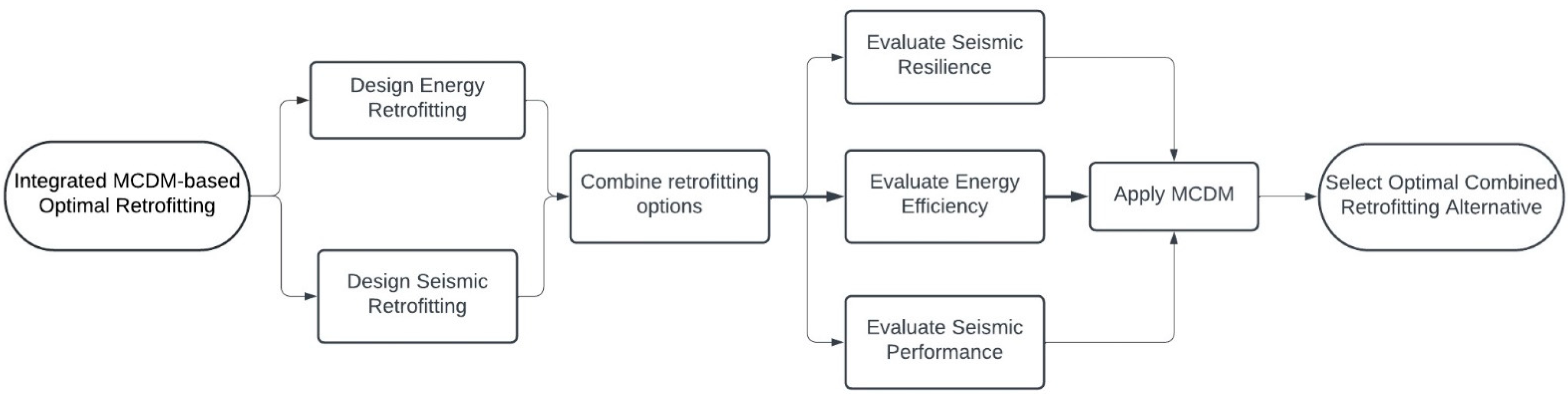
The integrated MCDM-based optimal retrofitting selection follows the procedure illustrated in the flowchart shown in Figure 15. The two first steps relate to designing the energy and seismic retrofitting separately. Then, the alternatives are combined to obtain a set of integrated energy and seismic retrofitting options. This new set of different retrofit combinations is evaluated in terms of energy efficiency, seismic performance, and seismic resilience. Finally, the MCDM is applied to the set of combined alternatives considering all the DVs of Table 5.

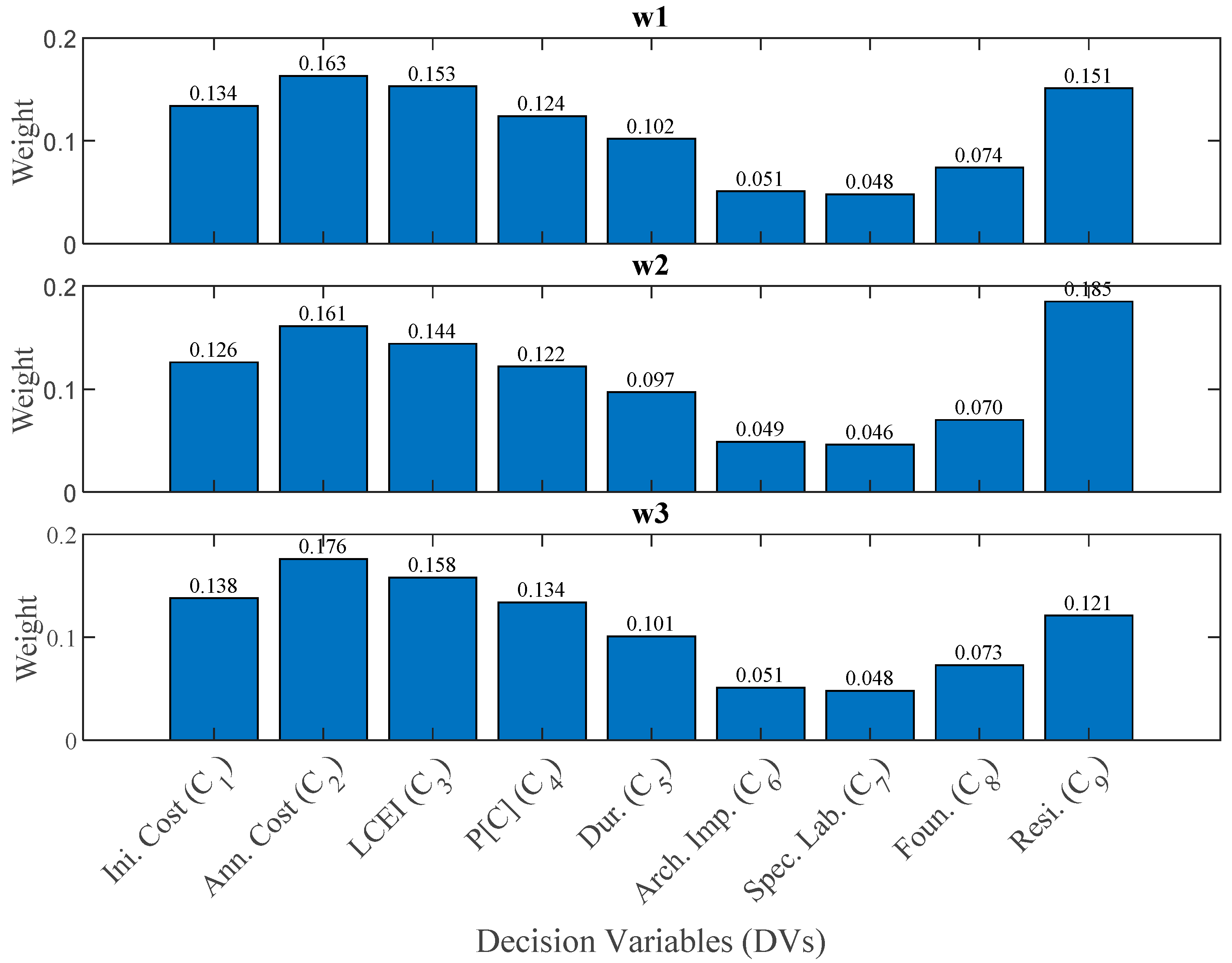
Regarding the weight vector (w) that is required for the MCDM implementation, one of many possible acceptable vectors was determined using the analytical hierarchy process (AHP) and engineering judgment. The same assumptions of Clemett et al. [30] guided the selection of the values for the pairwise comparison of the variables. Figure 16 illustrates three possible cases; w1 gives equal importance to the seismic resilience and LCEI (expected life cycle environmental impacts of retrofitted structure); w2 considers the seismic resilience as the most important parameter; w3 assumes seismic resilience as the fifth most important variable, with lower importance when compared to the annual probability of collapse but higher with respect to the duration of works.

Table 6. Decision variable values adopted from [30] and using three different seismic resilience parameters.

Model	C1 (EUR)	C2 (EUR)	C3 (kgCO2e)	C4	C5 (days)	C6	C7	C8	EARe	C9 Re_SLV	R1_SLD
S1E1	1,229,555	15.98	47.70	0.0019	61	0.023	0.084	5.71	4.35	43.90	0.94
S1E2	1,290,386	15.15	39.75	0.0018	61	0.023	0.084	5.71	4.36	43.90	0.94
S1E3	1,462,370	13.09	22.52	0.0018	65	0.023	0.084	5.71	4.36	43.90	0.92
S2E1	183,863	16.43	44.27	0.0044	22	0.056	0.013	16.54	4.24	43.90	0.93
S2E2	244,694	15.55	34.62	0.0040	24	0.056	0.013	16.54	4.24	43.90	0.92
S2E3	416,678	14.04	19.34	0.0043	29	0.056	0.013	16.54	4.23	43.90	0.92
S3E1	297,092	17.74	43.91	0.0027	42	0.093	0.084	16.61	4.29	45.20	0.94
S3E2	357,922	15.94	35.10	0.0024	42	0.093	0.084	16.61	4.33	43.90	0.93
S3E3	529,907	14.07	18.06	0.0027	46	0.093	0.084	16.61	4.33	43.90	0.94
S4E1	584,415	16.61	41.84	0.0008	44	0.162	0.151	4.77	4.42	94.40	1.00
S4E2	645,245	15.86	33.91	0.0008	44	0.162	0.151	4.77	4.42	94.50	1.00
S4E3	817,230	13.55	16.53	0.0008	48	0.162	0.151	4.77	4.44	94.40	1.00

represents the decision matrix used for conducting the MCDM analysis. The decision matrix was filled according to the results reported for the case study location (Isola del Gran Sasso, Italy), described in the study of Clemett et al. [30] (i.e., values for C₁ to C₈). The calculation of each DV value is described in detail by Clemett et al. [30]. To represent the seismic resilience DV (C₉), three parameters were considered, namely, the annualized resilience index (EARe), the resilience index at SLV (Re_SLV), and the ratio of all the building elements categorized with a repair class of 1 at SLD (R1_SLD).

The ranking representing the preference of all nine combined retrofitting strategies is reported in

Table 7. Rank using weight vector w1.

Model	Relative Closeness	Model	Relative Closeness	Model	Relative Closeness	Model	Relative Closeness
EARe		Re_SLV		Re_SLV		Clemett et al. [30]
S4E3	0.621	S4E3	0.646	S4E3	0.621	S4E3	0.633
S3E3	0.609	S4E2	0.633	S3E3	0.608	S4E2	0.617
S4E2	0.605	S4E1	0.608	S4E2	0.605	S4E1	0.595
S3E2	0.596	S3E3	0.543	S3E2	0.595	S3E3	0.592
S4E1	0.579	S3E2	0.533	S4E1	0.579	S3E2	0.570
S2E3	0.574	S2E3	0.527	S2E3	0.574	S2E3	0.561
S2E2	0.572	S2E2	0.526	S2E2	0.571	S3E1	0.558
S3E1	0.545	S3E1	0.500	S3E1	0.545	S2E2	0.523
S2E1	0.531	S2E1	0.496	S2E1	0.531	S2E1	0.517
S1E3	0.451	S1E3	0.422	S1E3	0.450	S1E3	0.455
S1E2	0.412	S1E2	0.382	S1E2	0.412	S1E1	0.420
S1E1	0.391	S1E1	0.364	S1E1	0.391	S1E2	0.420

when the weight vector w1 is used. Different tones of gray are used to distinguish the four seismic retrofitting options. On the other hand,

Table 8. Rank using weight vectors w2 and w3.

Model	Relative Closeness	Model	Relative Closeness	Model	Relative Closeness	Model	Relative Closeness
EARe_w2		R1_SLV_w2		EARe_w3		R1_SLV_w3
S4E3	0.624	S4E3	0.624	S4E3	0.629	S4E3	0.629
S4E2	0.608	S4E2	0.609	S4E2	0.613	S4E2	0.613
S3E3	0.605	S3E3	0.604	S3E3	0.610	S3E3	0.609
S3E2	0.594	S3E2	0.593	S3E2	0.597	S3E2	0.597
S4E1	0.582	S4E1	0.583	S4E1	0.586	S4E1	0.586
S2E3	0.566	S2E3	0.566	S2E3	0.565	S2E3	0.565
S2E2	0.565	S2E2	0.565	S2E2	0.564	S2E2	0.563
S3E1	0.543	S3E1	0.542	S3E1	0.544	S3E1	0.544
S2E1	0.525	S2E1	0.525	S2E1	0.523	S2E1	0.522
S1E3	0.455	S1E3	0.455	S1E3	0.455	S1E3	0.455
S1E2	0.418	S1E2	0.418	S1E2	0.416	S1E2	0.416
S1E1	0.397	S1E1	0.397	S1E1	0.394	S1E1	0.394

reports the cases for weight vectors w2 and w3 for the EARe and R1_SLD resilience DVs, since these are the seismic resilience DVs that alter the ranking preference of the second and third alternatives. All the tested options for weight vector and resilience DV resulted in S₄E₃ as the most beneficial strategy, which coincides with the selection reported in Clemett et al. [30]. However, the subsequent three preference positions follow the same pattern as in Clement et al. [30] just when Re_SLV is adopted as the seismic resilience parameter. For EARe and RI_SLD, S₃E₃, S₄E₂, and S₃E₂ are ranked as the second, third, and fourth best alternatives.

Furthermore, adopting different weight vectors slightly alters the rank positions of the alternatives with higher relative closeness, yet S₄E₃ is still granted the top position, i.e., as the most convenient solution. It is evident that by combining the strategy with CFRP and viscous dampers (seismic retrofitting) with the E₃ energy retrofitting level, the most favorable outcome is obtained.

5. Conclusions

This paper explored, for the first time, the use of seismic resilience parameters in an integrated assessment and evaluation of optimal seismic and energy retrofitting strategies for existing buildings. Initially, several methodologies were critically reviewed and scrutinized, highlighting the pros and cons of each approach, to determine the most practical parameter with which seismic resilience could be estimated. Such different methodologies were applied to a case study RC Italian school building with four retrofitting alternatives. Subsequently, resilience was integrated as an additional decision variable (DV) into a multicriteria decision-making (MCDM) framework that was employed to identify the optimal combination of seismic and energy-efficient retrofitting interventions for the case study building. The main conclusions that can be drawn about the role and impact of resilience in optimal retrofitting identification for existing buildings are as follows:

• Even though robustness is one metric of resilience, this parameter depends solely on expected economic losses. Robustness does not describe how recovery is carried out but rather indicates the remaining functionality of the building after a seismic event. On the other hand, rapidity integrates two parameters—losses and downtime. Therefore, rapidity is seen as a more precise parameter to estimate resilience, which gives an idea of how a building regains normal conditions throughout a recovery path;
• The resilience index is the most widely used method to measure resilience and corresponds to the integration of a functionality curve over the total downtime. The functionality curve is idealized by a linear, exponential, or trigonometric function, with the linear and trigonometric options often providing a closer approximation of the recovery path. However, when any of these functions is integrated, the resilience index does not vary much from one to another. Therefore, any of these functions can be assumed for estimating resilience indices, as part of other endeavors that do not have as the primary goal the estimation of resilience per se, such as a comparative analysis of different retrofitting alternatives;
• The Resilience-based Earthquake Design Initiative (REDi) Rating System was adopted not only as a rating system but also to estimate a particular recovery state. In such a case, the recovery path of a building is determined by adding the recovery cost of each repaired component (regaining functionality) and their repair time (downtime);
• Revising and conducting a critical analysis of the seismic resilience assessment methodologies available in the literature helped to identify the components that are suitable for determining the seismic resilience of buildings, which is not limited to the Italian context. Examining the pros and cos of each approach uncovered that an annualized expected resilience metric is more appropriate for the combined seismic and energy retrofitting framework;
• When carrying out the performance-based MCDM considering solely a resilience perspective, it was found that not conducting any intervention on the existing school building to improve its seismic resilience resulted in an extremely low relative closeness, meaning that this alternative is close to the negative solution of the worst possible case. This highlights the importance of improving the seismic resilience for deficient buildings and how a minimal improvement allows for a resilience increment, meaning that a building regains its operational capabilities much faster after a seismic event;
• Incorporating the seismic resilience into an MCDM framework, together with multiple other parameters, to select the optimal combination of seismic and energy-efficient retrofitting schemes, showed no effect on the identification of the most convenient strategy but modified the rank of the other alternatives. For all the three tested cases (i.e., granting seismic resilience the same importance as expected life cycle environmental impacts, assuming seismic resilience as the most important decision variable, and considering seismic resilience as the fifth most important variable), the retrofitting strategy based on CFRP and viscous dampers, combined with external wall insulation, replacement of windows with new double glazing with PVC frames with internal venetian blinds, and floor insulation, remained as the most convenient alternative. The reason for this is that such a retrofit strategy represents the most ideal solution for the DVs with the highest weights and, at the same time, leads to the best resilience improvement hence the relative closeness to the ideal solution remains close to one. Importantly, the rank of the retrofitting alternatives barely changed when other metrics of resilience were incorporated into the MCDM framework;
• Higher seismic resilience can be gained when all nonstructural elements are seismically retrofitted, in particular the ones that may compromise the normal operation of a building.

Some features of this study could be further improved when addressing the seismic resilience and selection of optimally integrated retrofitting. For instance, only one building was examined as a case study (school building occupancy type), and only one location was assessed for the seismic/climate conditions, whereas more locations with different seismic/climate settings would be useful. Furthermore, exploring a simplified procedure for estimating the seismic response (NLTHA) and loss assessment would make the framework more appealing for practitioners. Finally, this framework assumed that seismic retrofitting and energy retrofitting were carried out independently, whereas fully integrated solutions could be sought and analyzed.

References

1. Almufti, I.; Willford, M. REDi Rating System, Resilience-Based Earthquake Design Initiative for the Next Generation of Build-ings. Version 1.0. October 2013. Available online: https://static1.squarespace.com/static/61d5bdb2d77d2d6ccd13b976/t/61e85a429039460930278463/1642617413050/REDi_Final+Version_October+2013+Arup+Website+%288%29.pdf (accessed on 5 May 2021).
2. Hadigheh, S.A.; Mahini, S.S.; Setunge, S.; Mahin, S.A. A preliminary case study of resilience and performance of rehabilitated buildings subjected to earthquakes. Earthq. Struct. 2016, 11, 967–982. [Google Scholar] [CrossRef]
3. Thacher, T.D.; Pludowski, P.; Shaw, N.J.; Mughal, M.Z.; Munns, C.F.; Högler, W. Nutritional rickets in immigrant and refugee children. Public Health Rev. 2016, 37, 3. [Google Scholar] [CrossRef] [PubMed] [Green Version]
4. Tachibana, S.; Masuya, H.; Nakamura, S. Performance based design of reinforced concrete beams under impact. Nat. Hazards Earth Syst. Sci. 2010, 10, 1069–1078. [Google Scholar] [CrossRef] [Green Version]
5. Gaxiola-Camacho, J.R.; Azizsoltani, H.; Villegas-Mercado, F.J.; Haldar, A. A novel reliability technique for implementation of Performance-Based Seismic Design of structures. Eng. Struct. 2017, 142, 137–147. [Google Scholar] [CrossRef] [Green Version]
6. Terzic, V.; Merrifield, S.K.; Mahin, S. Lifecycle Cost Comparisons of Different Structural Systems; Structural Engineers Association of California: Berkeley, CA, USA, 2012. [Google Scholar]
7. Mayes, R.; Wetzel, N.; Tam, K.; Weaver, B.; Brown, A.; Pietra, D. Performance Based Design of Buildings to Assess and Minimize Damage and Downtime; New Zealand Society of Earthquake Engineering (NZSEE): Christchurch, New Zealand, 2013. [Google Scholar]
8. Ramirez, C.M.; Miranda, E. Significance of residual drifts in building earthquake loss estimation. Earthq. Eng. Struct. Dyn. 2012, 41, 1477–1493. [Google Scholar] [CrossRef]
9. Anwar, G.A.; Dong, Y. Seismic resilience of retrofitted RC buildings. Earthq. Eng. Eng. Vib. 2020, 19, 561–571. [Google Scholar] [CrossRef]
10. Cimellaro, G.P.; Reinhorn, A.M.; Bruneau, M. Seismic resilience of a hospital system. Struct. Infrastruct. Eng. 2010, 6, 127–144. [Google Scholar] [CrossRef]
11. Bruneau, M.; Chang, S.E.; Eguchi, R.T.; Lee, G.C.; O’Rourke, T.D.; Reinhorn, A.M.; Shinozuka, M.; Tierney, K.; Wallace, W.A.; Von Winterfeldt, D. A Framework to Quantitatively Assess and Enhance the Seismic Resilience of Communities. Earthq. Spectra 2003, 19, 733–752. [Google Scholar] [CrossRef] [Green Version]
12. Doost, D.M.; Pourabdollahtootkaboni, M.; Mahin, S.; Cimellaro, G.P. Development of a database for indicators of resilient systems. In Proceedings of the 16th World Conference on Earthquake, 16WCEE 2017, Santiago, Chile, 9–13 January 2017. [Google Scholar]
13. De Risi, R.; Sextos, A.; Zimmaro, P.; Simonelli, A.; Stewart, J. The 2016 Central Italy earthquakes sequence: Observations of incremental building damage. In Proceedings of the 11th National Conference in Earthquake Engineering, Earthquake Engi-neering Research Institute, Los Angeles, CA, USA, 25–29 June 2018. [Google Scholar]
14. Stewart, J.P.; Zimmaro, P.; Lanzo, G.; Mazzoni, S.; Ausilio, E.; Aversa, S.; Bozzoni, F.; Cairo, R.; Capatti, M.C.; Castiglia, M.; et al. Reconnaissance of 2016 Central Italy Earthquake Sequence. Earthq. Spectra 2018, 34, 1547–1555. [Google Scholar] [CrossRef] [Green Version]
15. EN 1998-1:2004; Eurocode 8: Design of Structures for Earthquake Resistance—Part 1: General Rules, Seismic Actions, and Rules for Buildings. The European Union: Brussels, Belgium, 2005.
16. EN 1998-3:2005; Eurocode 8: Design of Structures for Earthquake Resistance—Part 3: Assessment and Retrofit of Buildings. The European Union: Brussels, Belgium, 2005.
17. Norme Tecniche per le Costruzioni. DM 17/1/2018. Gazzetta Ufficiale della Repubblica Italiana; Italian Ministry of Infrastructure and Transport: Rome, Italy, 2018. [Google Scholar]
18. Mazzoni, S.; Castori, G.; Galasso, C.; Calvi, P.; Dreyer, R.; Fischer, E.; Fulco, A.; Sorrentino, L.; Wilson, J.; Penna, A.; et al. 2016–2017 Central Italy Earthquake Sequence: Seismic Retrofit Policy and Effectiveness. Earthq. Spectra 2018, 34, 1671–1691. [Google Scholar] [CrossRef]
19. Gazzetta Ufficiale. Ordinanza del Presidente del Consiglio dei Ministri 20 Marzo 2003 n.3274; Gazzetta Ufficiale della Repubblica Italiana No. 105; Gazzetta Ufficiale: Rome, Italy, 2003. [Google Scholar]
20. O’Reilly, G.J.; Perrone, D.; Fox, M.; Monteiro, R.; Filiatrault, A. Seismic assessment and loss estimation of existing school buildings in Italy. Eng. Struct. 2018, 168, 142–162. [Google Scholar] [CrossRef]
21. Perrone, D.; O’Reilly, G.J.; Monteiro, R.; Filiatrault, A. Assessing seismic risk in typical Italian school buildings: From in-situ survey to loss estimation. Int. J. Disaster Risk Reduct. 2019, 44, 101448. [Google Scholar] [CrossRef]
22. Blaser, A.R.; Starkopf, L.; Deane, A.M.; Poeze, M.; Starkopf, J. Comparison of Different Definitions of Feeding Intolerance: A Retrospective Observational Study. Clin. Nutr. 2015, 34, 956–961. [Google Scholar] [CrossRef] [PubMed]
23. Caruso, M.; Pinho, R.; Bianchi, F.; Cavalieri, F.; Lemmo, M. A Life Cycle Framework for the Identification of Optimal Building Renovation Strategies Considering Economic and Environmental Impacts. Sustainability 2020, 12, 10221. [Google Scholar] [CrossRef]
24. Roberto, G.; Carmine, G. Simplified seismic loss assessment for optimal structural retrofit of RC buildings. Earthq. Spectra 2021, 37, 346–365. [Google Scholar]
25. Leone, M.F.; Zuccaro, G. Seismic and energy retrofitting of residential buildings: A simulation-based approach. Seism. Energy Retrofit. Resid. Build. 2016, 1, 11–25. [Google Scholar]
26. Caterino, N.; Iervolino, I.; Manfredi, G.; Cosenza, E. Multi-Criteria Decision Making for Seismic Retrofitting of RC Structures. J. Earthq. Eng. 2008, 12, 555–583. [Google Scholar] [CrossRef]
27. Il Corriere Della SERA, 2016. Amatrice, Riprende L’anno Scolatico. Pronta la Nuova Scuola Nei Prefabbricati, 12 September. Available online: http://www.corriere.it/foto-gallery/cronache/16_settembre_12/amatrice-scuola-ricostruita-riapre-13-settembre-53eaeae8-78d8-11e6-a4665328024eb1f5.shtml (accessed on 11 February 2018).
28. Fiorentino, G.; Nuti, C.; Paolacci, F. Seismic response to 2016 Central Italy earthquakes of BRB retrofitted school building in Norcia. In Proceedings of the 16th World Conference on Earthquake Engineering, 16WCEE, Santiago, Chile, 9–13 January 2017. [Google Scholar]
29. Scislo, L.; Guinchard, M. COVID-19 lockdown impact on CERN seismic station ambient noise levels. Open Eng. 2022, 12, 62–69. [Google Scholar] [CrossRef]
30. Nicholas, C.; Carofilis Gallo, W.W.; Gabbianelli, G.; O’Reilly, G.J.; Monteiro, R. Optimal combined seismic and energy efficiency retrofitting for existing buildings. J. Struct. Eng. 2021, accepted. [Google Scholar]
31. Menna, C.; Del Vecchio, C.; Di Ludovico, M.; Mauro, G.M.; Ascione, F.; Prota, A. Conceptual design of integrated seismic and energy retrofit interventions. J. Build. Eng. 2021, 38, 102190. [Google Scholar] [CrossRef]
32. Formisano, A.; Vaiano, G.; Fabbrocino, F. Seismic and Energetic Interventions on a Typical South Italy Residential Building: Cost Analysis and Tax Detraction. Front. Built Environ. 2019, 5, 12. [Google Scholar] [CrossRef] [Green Version]
33. Passoni, C.; Marini, A.; Belleri, A.; Menna, C. Redefining the concept of sustainable renovation of buildings: State of the art and an LCT-based design framework. Sustain. Cities Soc. 2020, 64, 102519. [Google Scholar] [CrossRef]
34. Pohoryles, D.A.; Maduta, C.; Bournas, D.; Kouris, L.A.S. Energy performance of existing residential buildings in Europe: A novel approach combining energy with seismic retrofitting. Energy Build. 2020, 223, 110024. [Google Scholar] [CrossRef]
35. WCED. Report of the World Commission on Environment and Development. United Nations. 1987. Available online: https://www.are.admin.ch/dam/are/en/dokumente/nachhaltige_entwicklung/dokumente/bericht/our_common_futurebrundtlandreport1987.pdf.download.pdf/our_common_futurebrundtlandreport1987.pdf (accessed on 12 March 2022).
36. Benson, M.H.; Craig, R.K. The End of Sustainability: Resilience and the Future of Environmental Governance in the Anthropo-Cene; University Press of Kansas: Lawrence, KS, USA, 2017; p. 14. [Google Scholar]
37. Li, J.; Wang, T.; Shang, Q. Probability-based seismic resilience assessment method for substation systems. Struct. Infrastruct. Eng. 2020, 18, 71–83. [Google Scholar] [CrossRef]
38. Lu, X.; Liao, W.; Fang, D.; Lin, K.; Tian, Y.; Zhang, C.; Zheng, Z.; Zhao, P. Quantification of disaster resilience in civil engineering: A review. J. Saf. Sci. Resil. 2020, 1, 19–30. [Google Scholar] [CrossRef]
39. Kafali, C.; Grigoriu, M. Rehabilitation decision analysis. In Proceedings of the 9th International Conference on Structural Safety and Reliability, Rome, Italy, 19–23 June 2005. [Google Scholar]
40. Chang, S.E.; Shinozuka, M. Measuring Improvements in the Disaster Resilience of Communities. Earthq. Spectra 2004, 20, 739–755. [Google Scholar] [CrossRef]
41. Gallo, W.W.C.; Gabbianelli, G.; Monteiro, R. Assessment of Multi-Criteria Evaluation Procedures for Identification of Optimal Seismic Retrofitting Strategies for Existing RC Buildings. J. Earthq. Eng. 2021, 1–34. [Google Scholar] [CrossRef]
42. Eghbali, M.; Samadian, D.; Ghafory-Ashtiany, M.; Dehkordi, M.R. Recovery and reconstruction of schools after M 7.3 Ezgeleh-Sarpole-Zahab earthquake; part II: Recovery process and resiliency calculation. Soil Dyn. Earthq. Eng. 2020, 139, 106327. [Google Scholar] [CrossRef]
43. Samadian, D.; Ghafory-Ashtiany, M.; Naderpour, H.; Eghbali, M. Seismic resilience evaluation based on vulnerability curves for existing and retrofitted typical RC school buildings. Soil Dyn. Earthq. Eng. 2019, 127, 105844. [Google Scholar] [CrossRef]
44. O’Reilly, G.J.; Sullivan, T.J. Probabilistic seismic assessment and retrofit considerations for Italian RC frame buildings. Bull. Earthq. Eng. 2017, 16, 1447–1485. [Google Scholar] [CrossRef]
45. Elwood, K.J.; Marquis, F.; Kim, J.H. Post-earthquake assessment and repairability of RC buildings: Lessons from Canterbury and emerging challenges. In Proceedings of the Tenth Pacific Conference on Earthquake Engineering, Sydney, Australia, 6–8 November 2015. [Google Scholar]
46. Porter, K.A. An Overview of PEER’s Performance-Based Earthquake Engineering Methodology. In Proceedings of the Ninth Inter-national Conference on Applications of Statistics and Probability in Engineering, San Francisco, CA, USA, 6–9 July 2003. [Google Scholar]
47. FEMA P58-3. Seismic Performance Assessment of Buildings; Performance Assessment Calculation Tool (PACT), Version 2.9.65 (FEMA P-58-3.1); Applied Technology Council for the Federal Emergency Management Agency: Washington, DC, USA, 2012; Volume 3. [Google Scholar]
48. Anwar, G.A.; Dong, Y.; Li, Y. Performance-based decision-making of buildings under seismic hazard considering long-term loss, sustainability, and resilience. Struct. Infrastruct. Eng. 2020, 17, 454–470. [Google Scholar] [CrossRef]
49. Prota, A.; Di Ludovico, M.; Del Vecchio, C.; Menna, C. Progetto DPC-ReLUIS 2019-2021 WP5: Interventi di Rapida Esecuzione a Basso Impatto ed Integrati. RELUIS, 72. Recommended Lighting Levels in Buildings 2021. Archtoolbox.com. Available online: https://www.archtoolbox.com/materials-systems/electrical/recommended-lighting-levels-in-buildings.html (accessed on 27 July 2021).
50. Clemett, N.; Gallo, W.W.C.; O’Reilly, G.J.; Gabbianelli, G.; Monteiro, R. Optimal seismic retrofitting of existing buildings considering environmental impact. Eng. Struct. 2021, 250, 113391. [Google Scholar] [CrossRef]
51. Mackie, K.R.; Stojadinović, B. Comparison of Incremental Dynamic, Cloud, and Stripe Methods for Computing Probabilistic 908 Seismic Demand Models. In Structures Congress; ASCE: Reston, VA, USA, 2005; pp. 1–11. [Google Scholar]
52. Bradley, B.A. Practice-oriented estimation of the seismic demand hazard using ground motions at few intensity levels. Earthq. Eng. Struct. Dyn. 2013, 42, 2167–2185. [Google Scholar] [CrossRef] [Green Version]
53. Global Earthquake Model (GEM). The OpenQuake-Engine User Manual. Open-Quake Manual for Engine Version 3.7.0. 183. 2019. Available online: https://doi.org/10.13117/GEM.OPENQUAKE.MAN.ENGINE.3.7.0 (accessed on 15 October 2020).
54. Eads, L.; Miranda, E.; Lignos, D.G. Average spectral acceleration as an intensity measure for collapse risk assessment. Earthq. Eng. Struct. Dyn. 2015, 44, 2057–2073. [Google Scholar] [CrossRef]
55. Kohrangi, M.; Bazzurro, P.; Vamvatsikos, D.; Spillatura, A. Conditional spectrum-based ground motion record selection using average spectral acceleration. Earthq. Eng. Struct. Dyn. 2017, 46, 1667–1685. [Google Scholar] [CrossRef]
56. O’Reilly, G.J. Limitations of Sa(T1) as an intensity measure when assessing non-ductile infilled RC frame structures. Bull. Earthq. Eng. 2021, 19, 2389–2417. [Google Scholar] [CrossRef]
Figure 1. General components of resilience and main properties (4R) adapted from [10]. (a) Recovery function, (b) Robustness and Rapidity, (c) Resourcefulness, and (d) Redundancy.
Buildings 12 00845 g001
Figure 2. Typical model of seismic resilience using a recovery function.
Buildings 12 00845 g002
Figure 3. REDi recovery framework: (a) recovery states and (b) repair sequence, adapted from [1].
Buildings 12 00845 g003
Figure 4. Steps to estimate recovery time through REDi guidelines, Almufti and Willford 2013 [1].
Buildings 12 00845 g004
Figure 5. Example of repair sequence, considering delays and utility disruption, adapted from [1].
Buildings 12 00845 g005
Figure 6. Main modules of the proposed framework for PB–MCDM, adapted from [49].
Buildings 12 00845 g006
Figure 7. Illustration for computing EAC using a hazard curve and consequence curve, adapted from [49].
Buildings 12 00845 g007
Figure 8. Plan and elevation layout of the case study building.
Buildings 12 00845 g008
Figure 9. Hazard curve for the case study location and response acceleration spectrum for a return period of 712 years.
Buildings 12 00845 g009
Figure 10. Robustness of the case study school building (A0) and retrofitting alternatives.
Buildings 12 00845 g010
Figure 11. Rapidity of the case study school building (A0) and retrofitting alternatives.
Buildings 12 00845 g011
Figure 12. Recovery path for all models at Tr 712 years (SLV).
Buildings 12 00845 g012
Figure 13. Recovery path for all models at Tr 75 years (SLD).
Buildings 12 00845 g013
Figure 14. Seismic resilience index for a wide range of intensities using different recovery functions.
Buildings 12 00845 g014
Figure 15. Integrated MCDM-based optimal retrofitting selection methodology.
Buildings 12 00845 g015
Figure 16. Weight vectors for the MCDM analysis.
Buildings 12 00845 g016