Identifying Effective Managerial Factors in Improving and Renovating Old Urban Tissues: A Case Study Approach

Abstract

This paper attempts to identify the effective managerial factors in renovating old building tissues in a city in Iran (Langrud). The present research is practical in terms of purpose, and it is descriptive and contextual in terms of data collection. Furthermore, since this is a mixed research study from both the perspective of its nature and purpose, we conducted the study with both qualitative (interviews) and quantitative (questionnaires) methods. As the statistical population in the qualitative section consists of experts on improving worn-out tissues, we used an available sampling method and took into account the individuals’ characteristics in the sampling process. Seven managers, assistants, and engineers with more work experience than the rest of the managers and assistants were selected. During the quantitative phase, the population included all the municipality staff and the engineering system organization of Langrod city, which contains a total of 650 people. A total of 335 people were selected, and the questionnaire was distributed using Cochran’s formula. A semi-structured interview and a questionnaire were used as research tools distributed among participants. The validity and reliability of the questionnaires were determined based on existing standards. Additionally, the data were analyzed using Factor Analysis (FA), the Fuzzy Analytic Hierarchy Process (FAHP), and Structural Equations Modeling. According to the results, the most effective managerial factors and indicators in the improvement and renovation of the city’s old tissues were related to resources. Next, attention to training, commitment to environmental assessment, idea creation, planning, management, technical factors, experience, attention to legal requirements, and attention to external factors are placed.

1. Introduction

Improvements and renovations of urban areas have grown in importance in recent years [1,2,3]. The theory of sustainable urban development arose as a result of rapid scientific and technological developments, followed by a transformation of the social, economic, and physical structures of cities. As a result, urban improvement and renovation are among the most important topics in the 21st century and are of interest to various scientific fields. Worn-out urban tissues refer to areas within the legal boundaries of cities that have a low place, environmental, and economic value due to being physically worn-out, a lack of vehicle access, and a lack of public facilities, services, and urban infrastructures [4,5]. Due to the poverty of the residents and their owners, these areas cannot undergo spontaneous renovations, and investors are not motivated to invest in them [6]. As a result of aging and physical and functional wear-out, these areas fail to meet today’s needs. Consequently, these native populations migrate to the outskirts of the cities and are replaced by rural immigrants and low-income strata. These problems make these worn-out tissues even more in need of renovation and improvement. There are many dimensions to city improvement and renovation, including physical, social-cultural, economic, and political-administrative ones [7,8]. In other words, it is critical to preserve the identity and urban life when renovating and improving. A vital component of realizing the urban development policy from the inside is the improvement and modernization of worn-out urban tissues. However, this is a multifaceted, complex phenomenon with both physical and nonphysical dimensions [9]. Over time, all cities grow and evolve, and their texture changes as economic-social currents, weather conditions, and time pass. Depending on the geographical location and the cause of urban erosion, this transformation differs. When a city grows and develops and creates new spaces, the worn-out texture is reconstructed and improved by modern engineering principles, current conditions, and the local architecture. On the other hand, the historical identity of the city must also be preserved [10]. To improve and renovate an old and worn-out city’s fabric, it is necessary to conduct comprehensive investigations and research regarding climatology criteria, historical identity, management of the implementation of the improvement plan, contractor selection, employee commitment, cost control monitoring, and so on. It should also be done according to a detailed plan. Furthermore, paying attention to the culture, ecology, economy, and historical architecture of the city can greatly improve and renovate it [11].

Construction and renovation projects rely on effective managerial factors to succeed. The managers should consider the mentioned factors for improving the project level, eliminating obstacles, and using these factors to make the project successful. In today’s management and engineering fields, it has become increasingly common to identify effective managerial factors and use them in many projects, from military and defense projects to construction projects and infrastructure projects. We should pursue selecting some potentially effective factors in improving the management style and project quality. It is also imperative to pay attention to the target criteria and limitations in this subject area [12]. In addition, some criteria are critical in managing improvement and renovation projects. Making accurate decisions based on superior managerial indicators, selecting the right contractor, ensuring project implementation personnel’s commitment, controlling costs in the project, and adjusting the improvement model to the reality of the plan during implementation are just some of the factors that need to be considered. The preservation of local architecture, consideration of climate and weather variables, and other factors are also essential.

Identifying effective management factors is crucial to improving a country’s economic grade and civil status. In addition, enhancing and renovating worn-out buildings can be more successful when influential managerial factors are prioritized. Project management is so crucial that even the slightest error can lead to considerable losses, both financially and physically. Consequently, it is essential to identify and prioritize the most effective managerial factors for improving and renovating the old infrastructure of cities. However, various studies have been conducted on improving and renovating the old tissues of different Iranian cities. Despite this, no independent research has been accomplished on identifying influential managerial factors contributing to a successful renovation or improvement project. It is, therefore, necessary to work on this issue to manage improvement and renovation projects effectively. In addition, considering the number and types of these factors on the one hand, and the necessity of renovating and improving worn-out urban structures on the other, city managers should pay particular attention to these factors as they are crucial to improving and renovating cities. For example, we can indicate building and construction management factors that can improve project completion, monitoring, and control. To achieve several appropriate and effective indicators and factors that can improve the management level in multiple dimensions, we try to focus on the management of the proposed projects in improving and renovating the old tissues of Langrod. Therefore, according to the contents of this research, it seeks to answer the question of what is the prioritization of the effective management factors in the improvement and renovation of the old tissues of the city (case study: the city of Langrod) and which factor is more important? In addition, the objectives of the research are as follows:

General purpose: Prioritization of effective management factors in the improvement and renovation of the old tissues of the city (case study: Langrod city).

Sub-goals of the research:

✓

Identification of effective management factors in the improvement and renovation of the old tissues of Langrod city.

✓

Examining the contribution of each of the factors in the improvement and renovation of the old tissues of Langrod city.

✓

Presenting a model for ranking effective management factors in improving and renovating the old tissues of the city.

2. Research Background

During the research related to this topic, it was discovered that no independent study has been accomplished on investigating effective managerial factors for the improvement and renovation of old tissues of cities (case study: Langrod). Nevertheless, various studies have been conducted in different cities, some of which are listed here. Therefore, the contents of this section help to review the existing studies in this field in a brief way and to continue to improve this research direction.

It was stated by Mazraeh and Pazhouhanfar [13] that the architecture of Qeshm Island was unique to a hot and humid environment. Sustainable architecture and development are already goals of this architecture. Studies have not been conducted to identify the characteristics of native architecture and how they contribute to the island’s stability. As a result, we examined the island’s native architecture separately in three aspects: urban texture, single-base architecture, and architectural details. A quantitative study was conducted on 42 buildings over 70-years-old to document our analysis of the old texture of the city. Based on the results, it was concluded that factors such as beams, the thickness of walls, and openings play a critical role in the stability of Qeshm Island with regard to the urban texture, such as the structures of buildings, the framework of neighborhood spaces, and architectural details. Generally, the vernacular architecture of the island was based on an understanding of construction and an orientation toward the climate. Foroughi and Rasol [14] argue that housing is one of the most basic needs of all humans. It is crucial to renovate housing to ensure the quality and standards of living and to create the institution of urban planners and managers. When residents have a poor economic status, a high wear-out rate of residential units complicates the housing renewal process. Due to this, prioritization and preparation of plans for such renovations are considered according to the available resources.

As Trop [15] reports in his study, regeneration is happening in all occupied Palestinian cities, despite limited evaluation of social consequences. The results of a social impact assessment (SIA) for a demolition and reconstruction project of a low-income neighborhood last year are presented in this article. Using this research, they demonstrated that this project is a complete example of improvement, including the removal of dilapidated and small housing and its replacement with privately owned housing with better facilities and areas. They also gathered various points of view held by different public and private actors in this project to determine the actual and potential social consequences. Analyzing various documents, observing the reconstruction process on the ground, and conducting semi-structured interviews with key stakeholders and community representatives formed the basis of this study. Based on the results of that study, different methods approved in developed countries are more likely to improve project outcomes for all parties. In addition to promoting urban sustainability, SIAs could also improve strategic decision making within this particular type of regeneration. Vanvari and Mhaske [16] stated that many developing countries have old buildings that need to be developed and renovated. Renovating dilapidated, uneconomical, or rented buildings falls into this category. Since the last decade and a half, Mumbai has seen a lot of construction, development, and reconstruction. The process of renovating a structure or redevelopment project is quite complex due to some limitations and considerations. It takes a lot of time and effort to accomplish this. Several risks, uncertainties, and challenges exist in the Mumbai city development project that can lead to failure, causing great grief and loss to those involved. It is, therefore, vital to identify the risks and challenges that may arise during renovation projects. Interacting with all stakeholders involved in the Mumbai renovation project should enable researchers to demonstrate the risks of profit loss and the various problems and uncertainties. In a study examining the experiences of three old renovation periods in Guangzhou, Li et al. [17] concluded that residential development results in the loss of agricultural land and natural resources. Researchers and policymakers have expressed concern about this. Habitat III was founded by the United Nations in 2016 and encourages spatial development strategies to redevelop urban areas. It also describes methods for developing a new urban program using urban planning, context-oriented design, policies, rules, and regulations. Urban restructuring has become a reputation of the Chinese government. The land use policy for Guangzhou city has been analyzed in the context of three previous renovation experiences. Compared to the previous “top-down” approach, the policies and processes of the “three previous modernization periods” differed. This is because, in the second case, local governments should promote active participation from different stakeholders. Culture-based creativity is considered an important factor in the reconstruction of the three regions of China, as a catalyst for redefining the recognition of historical neighborhoods for reconstruction. In addition, the wisdom transfer approach can provide valuable lessons and experiences for other Chinese and developing cities; for more details, see [18,19,20,21,22,23,24,25].

3. Definitions of Terms and Concepts

3.1. Theoretical Definitions

Effective management factor: the action or factors that have influence on improving the management level of construction projects and have the highest priority.

Improvement and renovation of worn-out tissues: a set of measures that are carried out in order to renew buildings in damaged cities.

3.2. Operational Definitions

Effective managerial factor: In this research, 10 prominent factors obtained from the research background and semi-structured interview data, which were given the highest score by the people of the studied society (managers, assistants, engineers, and municipal employees, as well as the engineering system of the city of Langrod). These factors have more priority and a more effective role in the management of the improvement and renovation of worn-out tissues.

Improvement and renovation: In this research, the meaning of improvement and renovation is the reconstruction projects under the supervision of the municipality and the city’s engineering system.

3.3. Introducing the City of Langrod

Langrod is a city in Gilan province, between Lahijan and Rudsar, located in the north of Iran. Langrod is located at 30, 10, 50 longitudes and 11, 37 latitudes, at an altitude of 21 m above the Caspian Sea. There is a forest in the southern foothills of this city, which is situated on a green plain and 10 km away from the Caspian Sea. There is a 60 km distance between Langrod and Rasht (the province capital), and it connects the north with the Caspian Sea, the west with Lahijan, the east with Rudsar, and the south with Amlash. In 2015, Langrod city had a population of 140,686 according to the general population and housing census.

3.4. Research Scope (Temporal, Spatial, Subject)

The research period is winter and spring 2022. The spatial domain of the current research is on the construction companies that have been working in 2021–2022. Moreover, the subject area of this research is in the field of construction management research and construction companies.

4. Research Methodology

The current research has an applied purpose. Considering the nature and purpose of this study, mixed research methods were used, as well as descriptive and contextual data collection. The mixed-method research was conducted in two phases: qualitative (interviews) and quantitative (questionnaires).

4.1. The Qualitative Phase

A qualitative case study methodology was used for the qualitative part of the research. According to the research literature, ten components were extracted from the background information, and several sub-components were added for each. There were 35 sub-components, which were written in a table for judging in the qualitative phase. Qualitative data were collected from semi-structured interviews during the research phase. We asked those invited to the interview who were experts and opinionated people to rank the quantitative components and subcomponents based on their new opinions. Components and subcomponents were added or deleted in these opinions. This phase was qualitative due to the survey of Langrod municipality managers.

4.2. The Quantitative Phase

The research was conducted as a descriptive survey. The sample participants were asked to fill out the questionnaire that was created in the quantitative phase of the study. There are 650 people in the statistical population of the research, including managers, assistants, engineers, and employees of the municipal authority and the engineering system of Langrod and east of Gilan province. Since this study has two types of statistical populations (qualitative and quantitative phases), we used two types of sampling in this study, and since the statistical population for the qualitative portion of this study includes experts in Langrod’s improvement projects, sampling was conducted according to the available sampling method and the individual characteristics. Seven managers, assistants, and engineers with more work experience were selected (see

Table 1. Frequency of qualitative statistical population (semi-structured interview).

Population	Population Size (People)	Sample Size
Managers	20	5
Assistants	22	2
Total	42	7

).

In the quantitative phase of the research, 650 people are included in the statistical population, including managers, assistants, engineers, municipal employees, and engineering system employees of Langrod and east of Gilan province.

Cochran’s formula was used in this study to sample:

• n = sample size
• N = the size of the statistical population
• t or z = percentage of the standard error of the acceptable confidence factor
• p = a proportion of the population without a certain trait
• q = 1 − p = a proportion of the population without a certain trait
• d = degree of certainty or possible accuracy

We usually consider p and q as 0.5. The z value is usually 1.96. d can be 0.01 or 0.05.

$$\mathrm{n}=\frac{\frac{{\mathrm{z}}^2\mathrm{pq}}{{\mathrm{d}}^2}}{1+\frac{1}{\mathrm{N}}\left(\frac{{\mathrm{z}}^2\mathrm{pq}}{{\mathrm{d}}^2}-1\right)}$$

Based on the number of people in the research community and sampling using Cochran’s formula, 335 people were selected as the sample. As a result of the study on the sources and background of the interview, several components and sub-components were compiled. Semi-structured interviews were conducted with several professors and administrators to localize the components (see Figure 1).

Considering that the questionnaire has an Analytic Hierarchy Process (AHP), its target level is related to effective management factors in the improvement and renovation of old city tissues (case study: Langrod city).

To determine the validity and reliability of the questionnaire, the AHP method’s inconsistency rate (Cr) must be calculated for the matrix. If the inconsistency is within the permissible limit (Cr < 0.1), the questionnaire is sent back to the relevant statistical community for correction and feedback. Inconsistency rates of pairwise comparisons are monitored until they fall within acceptable limits.

One of the technical characteristics of measuring tools is their reliability. As mentioned, the concept pertains to how much the measurement tool gives the same results under the same circumstances. The correlation between repeated measurements under the same conditions is the test that determines the confidence coefficient (reliability). Cronbach’s alpha coefficient should be greater than 0.7 to ensure that the questionnaire is reliable enough to test the desired variables. Accordingly, in this study, professors and experts evaluate the questionnaire created, and validity is based on the opinions of professors, while reliability is based on the distribution of the questionnaire and Cronbach’s alpha coefficient in the Amos structural equation output. This research includes descriptive and inferential findings. Statistics, such as frequency distributions and percentages, are used in the descriptive section to describe the current situation of the studied society. Inferential analysis was performed using the AHP technique and collected data. In the first stage, components and questions were evaluated by using this method and distributing questionnaires to experts. At this stage, low-importance questions were removed from the questionnaire, and a final questionnaire was provided to the statistical sample. A structural equation method was then used to classify and test the research questions.

5. Data Analysis

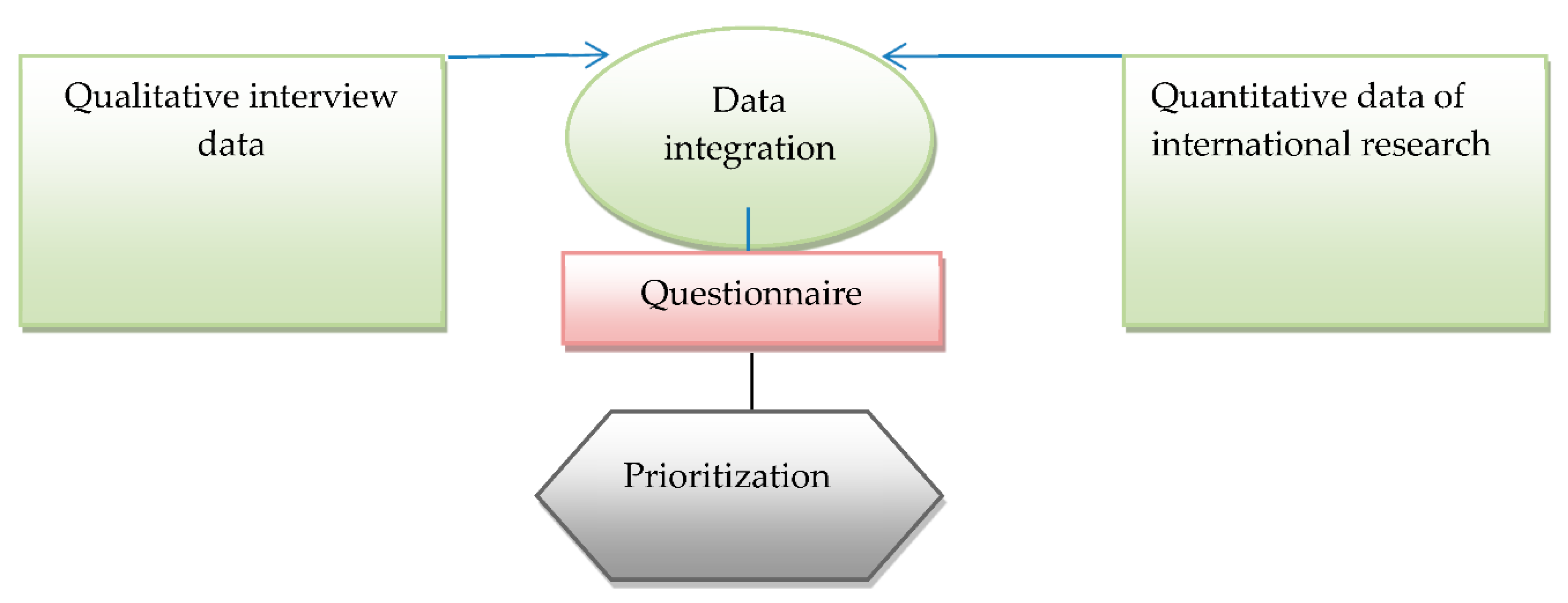
The purpose of this research is to rank the requirements and indicators of the improvement and renovation of the old tissues of the city through Analytical Hierarchy Process (AHP) techniques (case study: Langrod city). This technique involves constructing a hierarchical structure of the decision problem and then preparing a questionnaire (pairwise comparisons) containing some questions. Based on paired comparisons, this technique uses a matrix of paired comparisons, in which people compare two factors in pairs and rank one over the other by placing a number between 1 and 9. The purpose of a paired questionnaire was to compare the indicators and sub-indices of old city structures, as well as to identify and prioritize factors and indicators for improving and renovating them (case study: Langrod city). In the following paragraphs, we introduce the sub-indices. With the Analytic Hierarchy Process (AHP), several indicators are organized into a hierarchy. Decision making begins at the first level with the main goals. Indicators at the second level represent major and basic indicators (which can then be broken down into sub-indices). Optional decisions are presented at the last level.

• Level one: (decision’s objective):

The research aims to rank the factors and effective management indicators for the improvement and renovation of Langrod’s old tissues.

• Level two: (the main factors effective in the decision):

In this research, ten indicators have been selected as effective managerial factors in the improvement and renovation of the old tissues of Langrod city.

• Level three: the sub-components of each of the main factors effective in the decision:

Managerial indicators have seven sub-components in this study. Each of the technical indicators and the commitment to environmental assessment has three sub-components. There are four sub-components for indicators of resources, attention to training, and idea creation, and five sub-components for indicators of planning.

5.1. Questionnaire Integration (Normalization)

During this stage, we must integrate the 20 questionnaires collected before making pairwise comparisons. Ultimately, only one questionnaire should be collected. To calculate this, we use the geometric mean of the matrices, and the final questionnaire is the normalized matrix or matrix D, which is shown in

Table 2. Pairwise comparison matrix related to effective management factors and indicators in the improvement and renovation of old tissues of the city.

Matrix D Related to Effective Management Factors	Attention to Legal Requirements	Management	Technical	Resources	Attention to Training	Commitment to Environmental Assessment	Idea Creation	Planning	Attention to External Factors	Experience
Attention to legal requirements	1	0.9221	0.8798	0.7375	0.7459	0.7850	0.9923	0.7459	1.0134	0.8027
Management	1.0845	1	0.8941	0.8027	1.4811	0.8941	0.5920	0.5459	0.8941	1.4758
Technical	1.1367	1.1184	1	0.9696	0.8027	0.7402	0.8941	0.8027	0.7402	0.8941
Resources	1.3559	1.2457	1.0313	1	1.5047	0.9188	0.8472	1.3875	2.4927	2.2985
Attention to training	1.3406	0.6752	1.2457	0.6646	1	1.5047	1.6891	1.4727	1.3875	1.6667
Commitment to environmental assessment	1.2738	1.1184	1.3510	1.0884	1.2738	1	0.8342	1.6063	1.4811	0.8342
Idea creation	1.0077	1.6891	1.1184	1.1804	0.5920	1.1987	1	0.8941	1.3493	1.4811
Planning	1.3406	1.8317	1.2457	0.7207	0.6790	0.6226	1.1184	1	0.9696	1.0884
Attention to external factors	0.9867	1.1184	1.3510	0.4012	0.7207	0.6752	0.7411	1.0313	1	0.7784
Experience	1.2457	0.6776	1.1184	0.4351	0.6000	1.1987	0.6752	0.9188	1.2847	1
Total	11.7723	11.3967	11.2354	8.0002	9.4002	9.5380	9.3837	10.4053	12.6128	12.3200

.

As soon as we have formed the pairwise comparison matrix of indicators, we normalize their values. For this purpose, we divide each value of the matrix by the sum of its columns. For example, in the first column of the second row of Table 2:

$$\frac{1.0845}{11.7723}=0.0921 Output$$

We calculate the arithmetic mean of each row to calculate each index’s relative weight. The calculation results are given in

Table 3. The normalized matrix related to effective management factors and indicators in the improvement and renovation of the old tissues of the city.

Normalized Matrix	Attention to Legal Requirements	Management	Technical	Resources	Attention to Training	Commitment to Environmental Assessment	Idea Creation	Planning	Attention to External Factors	Experience
Attention to legal requirements	0.0849	0.0809	0.0783	0.0922	0.0794	0.0823	0.1058	0.0717	0.0804	0.0652
Management	0.0921	0.0877	0.0796	0.1003	0.1576	0.0937	0.0631	0.0525	0.0709	0.1198
Technical	0.0966	0.0981	0.0890	0.1212	0.0854	0.0776	0.0953	0.0771	0.0587	0.0726
Resources	0.1152	0.1093	0.0918	0.1250	0.1601	0.0963	0.0903	0.1333	0.1976	0.1866
Attention to training	0.1139	0.0592	0.1109	0.0831	0.1064	0.1578	0.1800	0.1415	0.1100	0.1353
Commitment to environmental assessment	0.1082	0.0981	0.1202	0.1360	0.1355	0.1048	0.0889	0.1544	0.1174	0.0677
Idea creation	0.0856	0.1482	0.0995	0.1475	0.0630	0.1257	0.1066	0.0859	0.1070	0.1202
Planning	0.1139	0.1607	0.1109	0.0901	0.0722	0.0653	0.1192	0.0961	0.0769	0.0883
Attention to external factors	0.0838	0.0981	0.1202	0.0501	0.0767	0.0708	0.0790	0.0991	0.0793	0.0632
Experience	0.1058	0.0595	0.0995	0.0544	0.0638	0.1257	0.0719	0.0883	0.1019	0.0812

and

Table 4. The priority of effective managerial factors and indicators in the improvement and renovation of the old tissues of the city.

Factors	Final Score	Priority
Attention to legal requirements	0.0821	9
Management	0.0917	6
Technical	0.0872	7
Resources	0.1306	1
Attention to training	0.1198	2
Commitment to environmental assessment	0.1131	3
Idea creation	0.1089	4
Planning	0.0994	5
Attention to external factors	0.0820	10
Experience	0.0852	8

.

As shown in Table 4 and the average of the factors, resources ranked highest among the effective managerial factors and indicators for improving and renovating the old tissues of the city. After that, the rankings are as follows: attention to training, commitment to environmental assessment, idea generation, planning, management, technical experience, attention to legal requirements, and attention to external factors. According to the answers of the experts and the priorities specified by them, it was decided to remove the indicators of experience, attention to legal requirements, and attention to external factors from the series of effective management factors in the final questionnaire to emphasize the importance of improving and renovating old tissues. The following section examines each of the approved component’s sub-indices. The process of prioritizing managerial indicators is shown in

Table 5. Pairwise comparison matrix related to management indicators.

Matrix D Related to Managerial Indicators	S1	S2	S3	S4	S5	S6	S7
Project Control	1	2.2513	2.4856	1.5121	0.7490	5.8845	1.0292
Materials management	0.4442	1	3.2439	1.9871	1.1689	3.3633	1.0649
Management skills	0.4023	0.3083	1	1.1789	1.8708	2.5581	1.4829
Ability and executive experience	0.6613	0.5032	0.8483	1	2.2938	2.6845	0.6010
Redefining the features and abilities and qualifications required by managers	1.3351	0.8555	0.5345	0.4360	1	1.8503	1.3493
Using experiences in the technical and professional field	0.1699	0.2973	0.3909	0.3725	0.5404	1	0.4443
Strengthening the theoretical and scientific capabilities of human resources	0.9716	0.9391	0.6743	1.6640	0.7411	2.2505	1
Total	4.9845	6.1547	9.1775	8.1506	8.3640	19.5914	6.9716

,

Table 6. Normalized matrix related to management indicators.

Matrix D Related to Managerial Indicators	S1	S2	S3	S4	S5	S6	S7
Project Control	0.2006	0.3658	0.2708	0.1855	0.0895	0.3004	0.1476
Materials management	0.0891	0.1625	0.3535	0.2438	0.1398	0.1717	0.1527
Management skills	0.0807	0.0501	0.1090	0.1446	0.2237	0.1306	0.2127
Ability and executive experience	0.1327	0.0818	0.0924	0.1227	0.2742	0.1370	0.0862
Redefining the features and abilities and qualifications required by managers	0.2679	0.1390	0.0582	0.0535	0.1196	0.0944	0.1935
Using experiences in the technical and professional field	0.0341	0.0483	0.0426	0.0457	0.0646	0.0510	0.0637
Strengthening the theoretical and scientific capabilities of human resources	0.1949	0.1526	0.0735	0.2042	0.0886	0.1149	0.1434

and

Table 7. Priority related to management indicators.

Indicators	Final Score	Priority
Project Control	0.2229	1
Materials management	0.1876	2
Management skills	0.1359	4
Ability and executive experience	0.1324	5
Redefining the features and abilities and qualifications required by managers	0.1323	6
Using experiences in the technical and professional field	0.0500	7
Strengthening the theoretical and scientific capabilities of human resources	0.1389	3

.

After that, there is the management of materials, strengthening the theoretical and scientific capabilities of human resources, management skills, power, and executive experience, redefining the characteristics, abilities, and qualifications required of managers, and utilizing technical and professional experiences. In accordance with the experts’ answers and their priorities, the sub-index of using technical and professional experiences was removed from the final questionnaire. The process of prioritizing technical indicators is shown in

Table 8. Pairwise comparison matrix related to technical indicators.

Matrix D Related to Technical Indicators	S8	S9	S10
Supply of machinery	1	3.0546	2.7589
Software capability	0.3274	1	1.2402
Engineering knowledge	0.3625	0.8063	1
Total	1.6898	4.8609	4.9992

,

Table 9. The normalized matrix related to the technical indicators.

Normalized Matrix	S8	S9	S10
Supply of machinery	0.5918	0.6284	0.5519
Software capability	0.1937	0.2057	0.2481
Engineering knowledge	0.2145	0.1659	0.2000

and

Table 10. Priority related to technical indicators.

Indicators	Final Score	Priority
Supply of machinery	0.5907	1
Software capability	0.2158	2
Engineering knowledge	0.1935	3

.

The highest ranking among the sub-indices of the technical factors is related to software power, based on the above table and factor averages. Then, there is the provision of machines and the knowledge of how engineers do their work. As a result of the experts’ answers and the priorities they specified, the sub-criterion of knowing how to do engineers’ work was eliminated from the final questionnaire. The process of prioritizing resource indicators can be seen in

Table 11. Pairwise comparison matrix related to resource indicators.

Matrix D Related to Resource Indicators	S11	S12	S13	S14
Technology use	1	1.4422	1.7904	0.7980
Initial estimates	0.6934	1	2.0056	1.0095
Funding	0.5585	0.4986	1	1.5697
Allocation of the necessary funds to prevent accidents	1.2532	0.9906	0.6371	1
Total	3.5051	3.9314	5.4330	4.3772

,

Table 12. The normalized matrix related to the resource indicators.

Normalized Matrix	S11	S12	S13	S14
Technology use	0.2853	0.3669	0.3295	0.1823
Initial estimates	0.1978	0.2544	0.3691	0.2306
Funding	0.1594	0.1268	0.1841	0.3586
Allocation of the necessary funds to prevent accidents	0.3575	0.2520	0.1173	0.2285

and

Table 13. Priority related to resource indicators.

Indicators	Final Score	Priority
Technology use	0.2910	1
Initial estimates	0.2630	2
Funding	0.2072	4
Allocation of the necessary funds to prevent accidents	0.2388	3

.

According to the table above and the average of all the factors, the use of technology ranked highest among the indicators of the resource factors. After that, there are initial estimates, the allocation of necessary funds for the prevention of accidents, and funding. According to the answers of the experts and the priorities specified by them, the subject of funding is removed from the final questionnaire.

Table 14. Pairwise comparison matrix related to attention to training indicators.

Matrix D Related to Training Indicators	S15	S16	S17	S18
Updating technician skills	1	0.8599	0.4413	0.5132
Utilizing academic elites	1.1629	1	2.2731	0.8291
Workshops on technical and skill development	2.2660	0.4399	1	0.9642
Using the world’s current knowledge to train technicians	1.9486	1.2061	1.0371	1
Total	6.3774	3.5059	4.7515	3.3065

,

Table 15. The normalized matrix related attention to training indicators.

Matrix D Related to Training Indicators	S15	S16	S17	S18
Updating technician skills	0.1568	0.2453	0.0929	0.1552
Utilizing academic elites	0.1823	0.2852	0.4784	0.2508
Workshops on technical and skill development	0.3553	0.1255	0.2105	0.2916
Using the world’s current knowledge to train technicians	0.3055	0.3440	0.2183	0.3024

and

Table 16. Priority related to attention to training indicators.

Indicators	Final Score	Priority
Updating technician skills	0.1625	4
Utilizing academic elites	0.2992	1
Workshops on technical and skill development	0.2457	3
Using the world’s current knowledge to train technicians	0.2926	2

illustrate how the indicators of attention to training in improvement activities is prioritized.

Based on the above table and the average of the factors, utilizing academic elites ranked highest among the attention to training criterion. Then, using the world’s current knowledge to train technicians, holding workshops on technical and skill development, and updating technician skills are placed next. In the final questionnaire, updating technician skills was removed based on the answers of the experts.

Table 17. Pairwise comparison matrix related to commitment to environmental assessment indicators.

Matrix D Related to Commitment to Environmental Assessment Indicators	S19	S20	S21
The reduction of environmental damage	1	2.6158	1.0065
Developing environmental strategies	0.3823	1	0.4472
Reduction of risks and environmental threats in improvement	0.9936	2.2361	1
Total	2.3759	5.8519	2.4537

,

Table 18. The normalized matrix related to attention to commitment to environmental assessment indicators.

Matrix D Related to Commitment to Environmental Assessment Indicators	S19	S20	S21
The reduction of environmental damage	0.4209	0.4470	0.4102
Developing environmental strategies	0.1609	0.1709	0.1823
Reduction of risks and environmental threats in improvement	0.4182	0.3821	0.4075

and

Table 19. Priority related to attention to commitment to environmental assessment indicators.

Indicators	Final Score	Priority
The reduction of environmental damage	0.1625	1
Developing environmental strategies	0.2992	3
Reduction of risks and environmental threats in improvement	0.2926	2

illustrate the process for prioritizing the indicators related to commitment to environmental assessment.

Based on the above table, the reduction of environmental damages ranked highest. After that, there are two indicators of developing environmental strategies and the reduction of risks and environmental threats in the improvement. In the final questionnaire, the risk reduction and threats to improvement plans for the environment were removed based on the experts’ responses and priorities.

In

Table 20. Pairwise comparison matrix related to idea creation indicators.

Matrix D Related to Idea Creation Indicators	S22	S23	S24	S25
Project goals’ clarity	1	0.4670	5.3566	5.5555
Explanation of conditions, limitations, and available possibilities	2.1411	1	7.0168	6.9035
Paying attention and checking the employees’ new ideas	0.1867	0.1425	1	2.3305
Creating a research team and studying scientific research on improving the old tissues	0.1800	0.1449	0.4291	1
Total	3.5078	1.7544	13.8025	15.7895

,

Table 21. The normalized matrix related to idea creation indicators.

Matrix D Related to Idea Creation Indicators	S22	S23	S24	S25
Project goals’ clarity	0.2851	0.2662	0.3881	0.3518
Explanation of conditions, limitations, and available possibilities	0.6104	0.5700	0.5084	0.4372
Paying attention and checking the employees’ new ideas	0.0532	0.0812	0.0725	0.1476
Creating a research team and studying scientific research on improving the old tissues	0.0513	0.0826	0.0311	0.0633

and

Table 22. Priority related to attention to idea creation indicators.

Indicators	Final Score	Priority
Project goals’ clarity	0.3228	2
Explanation of conditions, limitations, and available possibilities	0.5315	1
Paying attention and checking the employees’ new ideas	0.0886	3
Creating a research team and studying scientific research on improving the old tissues	0.0571	4

, we show the process of prioritizing the indicators of idea creation.

According to the table above and the average of all the factors, explanation of conditions, limitations, and available possibilities ranked highest among the indicators of idea creation. After that, there are project goals’ clarity, paying attention and checking the employees’ new ideas, and creating a research team and studying scientific research on improving the old tissues. According to the answers of the experts and the priorities specified by them, the subject of “creating a research team and studying scientific research on improving the old tissues” was removed from the final questionnaire.

Table 23. Pairwise comparison matrix related to planning indicators.

Matrix D Related to Planning Indicators	S26	S27	S28	S29	S30
Pay attention to the quality control unit	1	1.3636	0.6632	1.5747	0.9603
Use of experienced technicians	0.7334	1	1.7964	0.7059	1.1953
Addressing needs	1.5078	0.5567	1	1.1698	0.6544
Managers’ incentives/penalties	0.6350	1.4166	0.8548	1	1.2227
Realistic timing	1.0414	0.8366	1.5281	0.8179	1
Total	4.9176	5.1735	5.8425	5.2683	5.0326

,

Table 24. The normalized matrix related planning indicators.

Matrix D Related to Planning Indicators	S26	S27	S28	S29	S30
Pay attention to the quality control unit	0.2034	0.2636	0.1135	0.2989	0.1908
Use of experienced technicians	0.1491	0.1933	0.3075	0.1340	0.2375
Addressing needs	0.3066	0.1076	0.1712	0.2221	0.1300
Managers’ incentives/penalties	0.1291	0.2738	0.1463	0.1898	0.2430
Realistic timing	0.2118	0.1617	0.2615	0.1552	0.1987

and

Table 25. Priority related to attention to planning indicators.

Indicators	Final Score	Priority
Paying attention to the quality control unit	0.2140	1
Use of experienced technicians	0.2043	2
Addressing needs	0.1875	5
Managers’ incentives/penalties	0.1964	4
Realistic timing	0.1978	3

illustrate how planning indicators are prioritized.

According to Table 25 and the average of all the factors, paying attention to the quality control unit ranked highest among the indicators of planning. After that, there are the use of experienced technicians, realistic timing, managers’ incentives/penalties, and addressing needs. According to the answers of the experts and the priorities specified by them, addressing needs was removed from the final questionnaire.

5.2. Determining Inconsistency Rate

To determine whether our pairwise comparisons are consistent, the inconsistency rate should be calculated. The inconsistency rate is calculated only for pairwise comparisons of factors. We should perform this operation for each criterion’s indicator. As a first step, we multiply the initial integrated matrix (D) by the average of the same matrix to obtain the weighted sum vector. This is the product of pairwise comparisons of indicators in the relative weight vector. That means:

$$\mathrm{WSV}=\mathrm{DW},$$

where W represents relative weight, D represents the initial integral matrix, and WSV represents the weighted sum vector. The next step is to divide the result (WSV) by the index’s relative weight vector to obtain the compatibility vector (cv). Lastly, we obtain the arithmetic mean of the above vectors (compatibility CV), which is called λ_max. The calculated λ_max related to the components of the factors is specified in

Table 26. The factors’ λ_max.

Factors	λmax
Effective managerial factors in improving and renovating old urban structures	10.3789
Management	7.6269
Technical	3.0112
Resources	4.2236
Attention to training	4.2132
Commitment to environmental assessment	3.0025
Idea creation	4.1256
Planning	5.2352

.

As a fourth step, we calculate the inconsistency index (II) based on the following relationships:

$$\mathrm{II}=\frac{{\mathsf{\lambda }}_{\max }-\mathrm{n}}{\mathrm{n}-1},$$

$$\mathrm{IR}=\frac{\mathrm{II}}{\mathrm{IIR}},$$

The IIR is calculated from

Table 27. IIR figures.

10	9	8	7	6	5	3	3	2	1	n
1.51	1.45	1.41	1.32	1.24	1.12	0.9	0.58	0	0	IRI

.

The inconsistency rate of all components is shown in

Table 28. The factors’ inconsistency rate.

Factors	Inconsistency Index (IR)
Effective managerial factors in improving and renovating old urban structures	0.0279
Management	0.0792
Technical	0.0097
Resources	0.0828
Attention to training	0.0790
Commitment to environmental assessment	0.0022
Idea creation	0.0465
Planning	0.0474

.

There is acceptable consistency in the pairwise comparisons since all factors have an IRI of less than 0.1. Based on the examples and experts’ opinions, the low-importance questions were removed from the final questionnaire, which was provided to the statistical sample for purification and analysis.

5.3. Research Descriptive Findings

In this section, the statistical population for the second part of the research (creating the structural equation model) includes approximately 650 managers and employees related to the improvement of the old texture in Langrod, 335 of whom were selected for research based on the explanations given in Section 4. Using the output of SPSS software, we first draw the tables and graphs using the response data from the first part of the research questionnaire. The characteristics of an individual include marital status, age, job position, and education. The current study examines first the sample distribution of the marital status variable.

According to

Table 29. Frequency distribution of marital status in the sample.

Qualitative Variable	Level	Frequency	Frequency Percentage	Cumulative Percentage
Marital status	Single	53	15.82	15.82
	Married	282	84.18	100
	Total	335	100

, the marital status of the statistical sample under study is classified into two levels.

Based on the statistical sample studied,

Table 30. Frequency distribution of age in the sample.

Qualitative Variable	Level	Frequency	Frequency Percentage	Cumulative Percentage
Age	20 to 30 years old	91	27.16	27.16
	31 to 40 years old	166	49.55	76.72
	41 to 50 years old	46	13.73	90.45
	Above 51 years old	32	9.55	100
	Total	335	100

shows the multi-level age variable.

In

Table 31. Frequency distribution of job position in the sample.

Qualitative Variable	Level	Frequency	Frequency Percentage	Cumulative Percentage
Job position	Managers	19	5.67	5.67
	Assistants	21	6.27	11.94
	Engineers	74	22.09	34.03
	Staff	221	65.97	100
	Total	335	100

, the multi-level variable of the job position is shown in its current status.

SPSS software produces descriptive findings about research variables, which are interpreted and analyzed descriptively. The descriptive findings include the central index (mean), dispersion indices (standard deviation and range of changes), and skewness–stretch distribution indices. An analysis of

Table 32. Central indices and dispersion of variables related to research factors.

Variables	Number	Range of Changes	The Least Amount	The Highest Amount	Average	Standard Error of the Mean
Management	335	3.67	1.33	5	3.0846	0.03553
Technical	335	4	1	5	3.4537	0.04713
Resources	335	4	1	5	3.3970	0.04161
Attention to training	335	3	2	5	3.4627	0.03385
Commitment to environmental assessment	335	3.5	1.5	5	3.1030	0.04219
Idea creation	335	3.33	1.67	5	3.3831	0.03518
Planning	335	3	2	5	3.3627	0.03035
Effective managerial factors	335	2.63	2.1	4.73	3.3210	0.02429

shows the central and dispersion indicators related to the factors that improve and renovate old tissues of a city (case study: Langrod).

For the operational definition of variables, average questions have been used, as shown in Table 32. In the improvement and renovation of the old tissues of Langrod city, the minimum range of changes for the variable of effective management criteria and indicators is equal to 2.63, while the maximum range of changes for the variables of resources and technical factors is equal to 4. Furthermore, the mean scores of the variables are greater than 3 (the average of the five-point Likert scale), which indicates respondents’ preference for high, medium, and very high options.

In

Table 33. The indicators of distribution of variable observations related to research factors.

Variables	Number	Standard Deviation	Crookedness	Standard Error of the Deviation	Elongation
Management	335	0.65036	0.122	0.133	0.145
Technical	335	0.86262	−0.430	0.133	0.165
Resources	335	0.76164	−0.352	0.133	−0.248
Attention to training	335	0.61948	0.297	0.133	0.401
Commitment to environmental assessment	335	0.77227	0.245	0.133	0.065
Idea creation	335	0.64396	0.213	0.133	−0.093
Planning	335	0.55548	−0.049	0.133	−0.582
Effective managerial factors	335	0.44465	0.298	0.133	0.584

, effective managerial factors in improving and renovating old city tissues are outlined.

With a skewness coefficient based on the research findings, Table 33 shows the highest standard deviation is related to technical factors, indicating the greater dispersion of this component compared to other components. The lowest standard deviation is related to the component of effective managerial indicators, and the dispersion related to this component is also the lowest. Being less than 0.5 indicates that the data distribution is close to normal. To check the distribution of data, the Kolmogorov–Smirnov test is used.

The research variables were tested for normality using the Kolmogorov–Smirnov method. Kolmogorov–Smirnov statistics and significance levels for the research variables are shown in

Table 34. The result of the Kolmogorov–Smirnov test of research variables.

Variables	Number	Average	Standard Deviation	Test Statistics	The Significance Level
Management	335	3.0846	0.65036	0.089	0.064
Technical	335	3.4537	0.86262	0.164	0.122
Resources	335	3.3970	0.76164	0.125	0.112
Attention to training	335	3.4627	0.61948	0.147	0.129
Commitment to environmental assessment	335	3.1030	0.77227	0.186	0.062
Idea creation	335	3.3831	0.64396	0.145	0.095
Planning	335	3.3627	0.55548	0.111	0.051
Effective managerial factors	335	3.3210	0.44465	0.044	0.2

.

The Kolmogorov–Smirnov test statistic indicates that the data have a normal distribution and the significance level is greater than 0.05.

5.4. Validity and Reliability of the Questionnaire

To assess the structural validity of the spectra, factor analysis was also used as part of the theoretical foundations. By using this method, a large set of variables can be reduced to a smaller set of factors [26,27,28]. As the variables used in the current research have strong theoretical bases, the confirmatory factor analysis method was used to test the factorial structure of the mentioned model in the test plant. Consequently, in the following, we briefly describe the confirmatory factor analysis. The accuracy of the measurement of the structures is examined in this section by using structural equation modeling measurement models. By using factor analysis, it is determined whether the questions designed in each construct can measure the desired construct. Essentially, it determines whether the questions and indicators considered have the necessary validity. Confirmatory factor analysis presents standard coefficients and significant coefficients. Factor loading indicates the strength of the relationship between a factor (hidden variable) and an observable variable. A factor load is a value between 0 and 1. Weak relationships are considered when the factor load is less than 0.3, acceptable relationships are between 0.3 and 0.6, and favorable relationships are greater than 0.6.

Path coefficients or standard factor loadings between factors and markers are expressed by standardized coefficients. Validity requires a significant correlation between each construct and its indicators. Correlations are measured by significant values. Each parameter’s significance is shown by a significant number or t-value. The model parameters are significant if their value is greater than 1.96. In the factor model of the present research, all the values of the standard coefficients are higher than 0.3, which indicates that the factor model is appropriate and questions do not need to be removed. The standard factor loadings and significant coefficients of the questions are shown in

Table 35. The results of the confirmatory factor analysis of the questionnaire.

Variable	Indicator	Standard Factor Load	T-Value	Cronbach’s Alpha
Management				0.735
	Project Control	0.619
	Materials management	0.529	7.391
	Management skills	0.703	8.771
	Ability and executive experience	0.652	8.386
	Redefining the features and abilities and qualifications required by managers	0.654	7.738
	Strengthening the theoretical and scientific capabilities of human resources	0.300	4.720
Technical				0.821
	Supply of machinery	0.805
	Software capability	0.863	14.962
Resource				0.710
	Technology use	0.742
	Initial estimates	0.781	10.553
	Allocation of the necessary fund to prevent accidents	0.674	9.286
Attention to Training				0.772
	Utilizing academic elites	0.839
	Workshops on technical and skill development	0.538	8.365
	Using the world’s current knowledge to train technicians	0.724	9.381
Commitment to environmental assessment				0.703
	The reduction of environmental damage	0.711
	Reduction of risks and environmental threats in improvement	0.764	11.644
Idea Creation				0.863
	Project goals’ clarity	0.651
	Explanation of conditions, limitations, and available possibilities	0.715	8.821
	Paying attention and checking the employees’ new ideas	0.539	5.806
Planning				0.770
	Paying attention to the quality control unit	0.741
	Use of experienced technicians	0.658	9.836
	Managers’ incentives/penalties	0.490	7.037
	Realistic timing	0.656	9.454

. All of them indicate that the questions have appropriate factor loadings and their significant coefficients are also significant. For each variable, Cronbach’s alpha values were calculated, which were all above 0.7, indicating the questionnaire is reliable.

Table 36. Acceptable threshold and observed values of fit indices in the questionnaire.

Index Name	Recommended Amount	The Value Observed in the Present Study
Root-Mean-Square Error of Approximation (RMSEA)	Less than 0.8	0.729
Softened Fit Index (NFI)	More than 0.9	0.966
Comparative Fit Index (CFI)	More than 0.9	0.949
Goodness of fit index (GFI)	More than 0.9	0.83
Adjusted Goodness of Fit Index (AGFI)	More than 0.8	0.937

summarizes the recommended values and observed values of the fit indices. It is equal to 158/596 in the chi-squared test. With a significance level of 0.0001, it is significant at a confidence level of 99%. This value indicates the low fit of the model. There are 2.688 degrees of freedom in the presented research model, which is within the allowed range. We obtained an RMSEA value of 0.729, which is smaller than the recommended value of 0.8, indicating that the model fits the data well. An incremental fit index (IFI) equals 0.961, a normalized fit index (NFI) equals 0.966, a comparative fit index (CFI) equals 0.949, a goodness of fit index (GFI) equals 0.83, and an adjusted goodness of fit index (AGFI) equals 0.937. As a result, the fit indices are at the optimal level, indicating that the model is appropriately fitted.

6. Conclusions

Effective management factors in improving and renovating the old tissues of a city are critical factors in an organizational process or construction project. Managers should focus on improvement projects and their processes, which is what this research aims to do. This research aimed to identify and prioritize effective managerial factors necessary to improve and renovate the old tissues of Langrod. Mixed research methods were used to identify effective managerial factors for improving and renovating the old tissues of Langrod city. Since the research method was mixed, two phases, one qualitative (interviews) and one quantitative (questionnaires), were conducted. According to the results, resources ranked highest among the effective managerial criteria and indicators in improving and renovating old tissues. Then, education, commitment to environmental assessment, idea creation, planning, management, technical, experience, legal requirements, and, finally, external factors are addressed. The problems and limitations of the research can be mentioned here. The newness of the subject and lack of sufficient resources were the difficulties, which of course became clear at the beginning of the subject selection and preliminary studies. Unfortunately, the uncoordinated and lackluster communication of the employees and managers showed up many times and showed their indifference towards the research work, and the weakness of this communication in the distribution and collection of questionnaires was very clear, because the need for face-to-face communication showed that the language of this communication is very weak.