
Evaluation of ALARO-0 and REMO Regional Climate Models over Iran Focusing on Building Material Degradation Criteria

 , ,
, ,
Abstract
:1. Introduction
2. Materials and Methods
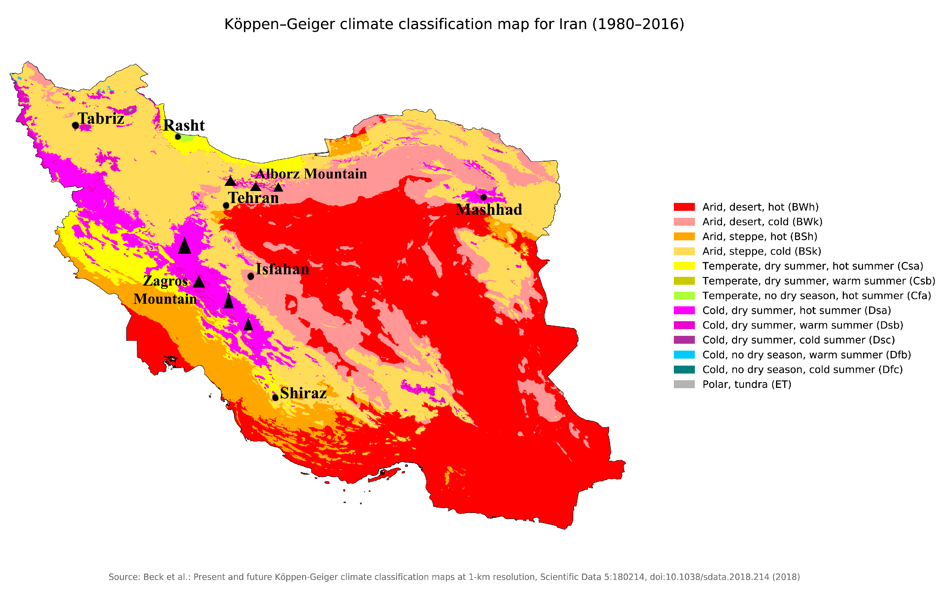
2.1. Study Area
2.2. Model Description and Experimental Design
2.3. Method of Analysis
2.3.1. Statistical Analysis
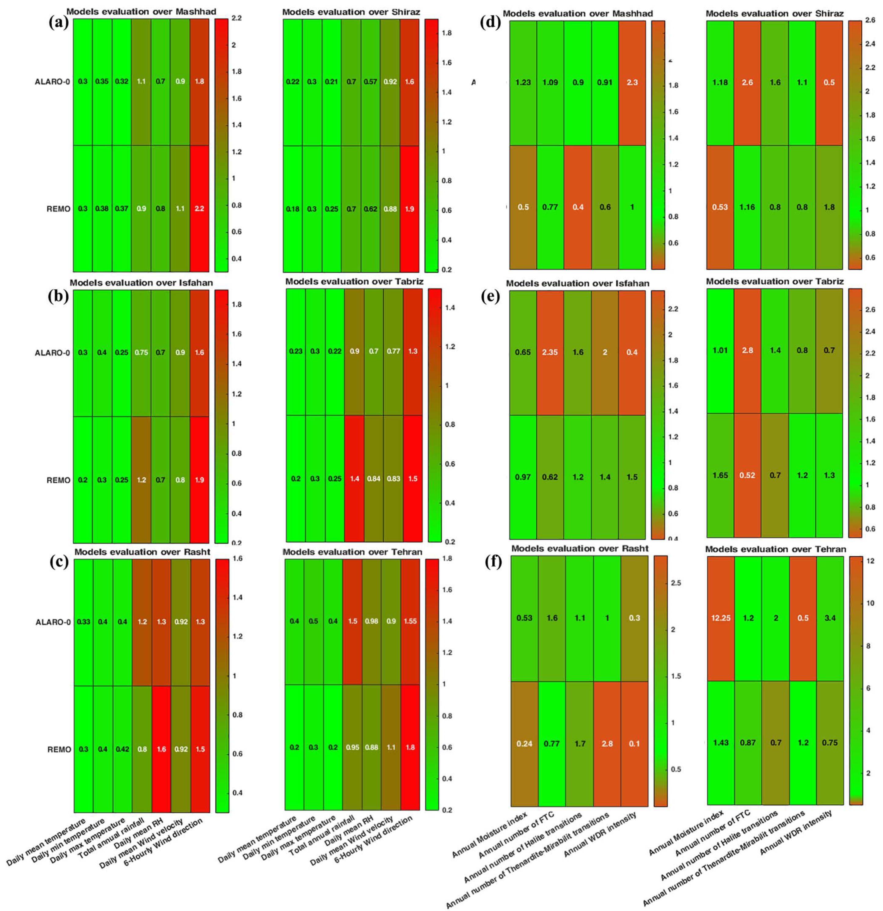
2.3.2. Scoring Methodology
2.3.3. Calculation of Indices
Freeze–Thaw Cycles (FTCs)
Salt Crystallisation
Moisture Index (MI)
Wind-Driven Rain (WDR)
3. Results
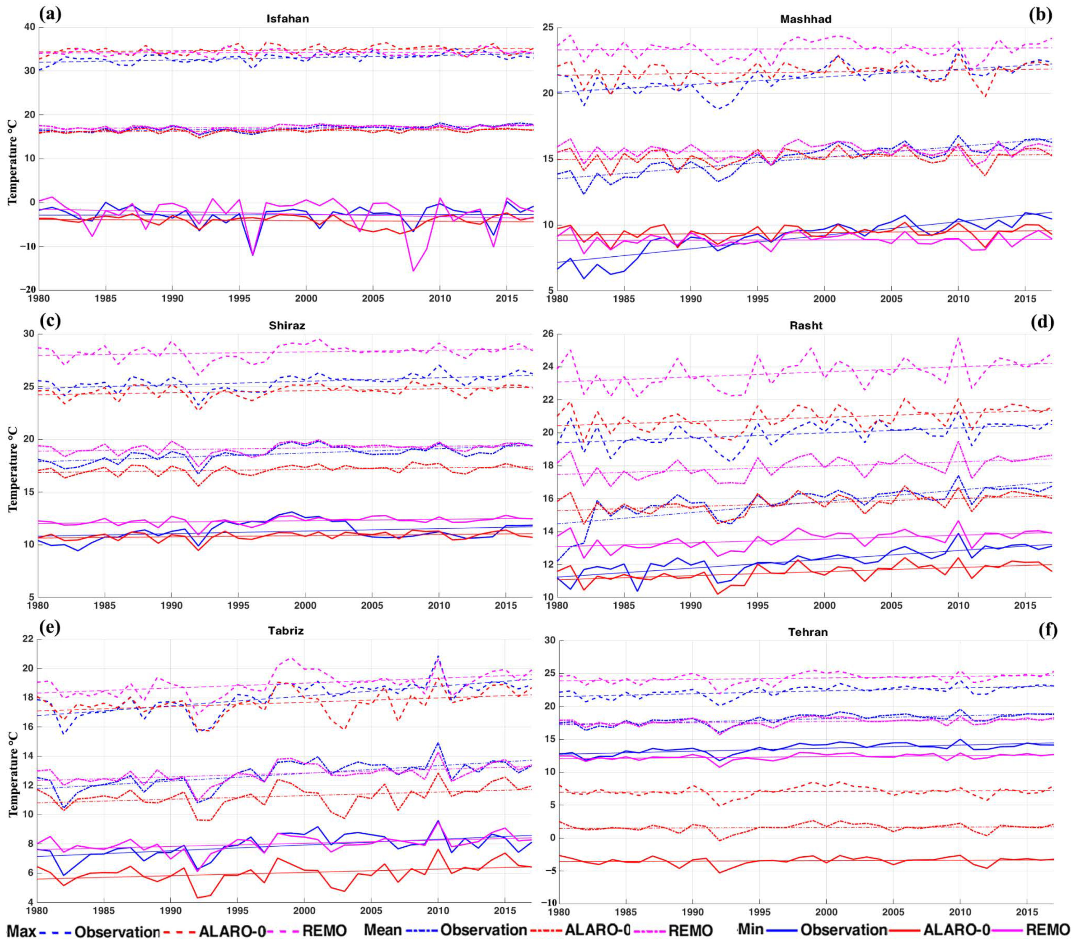
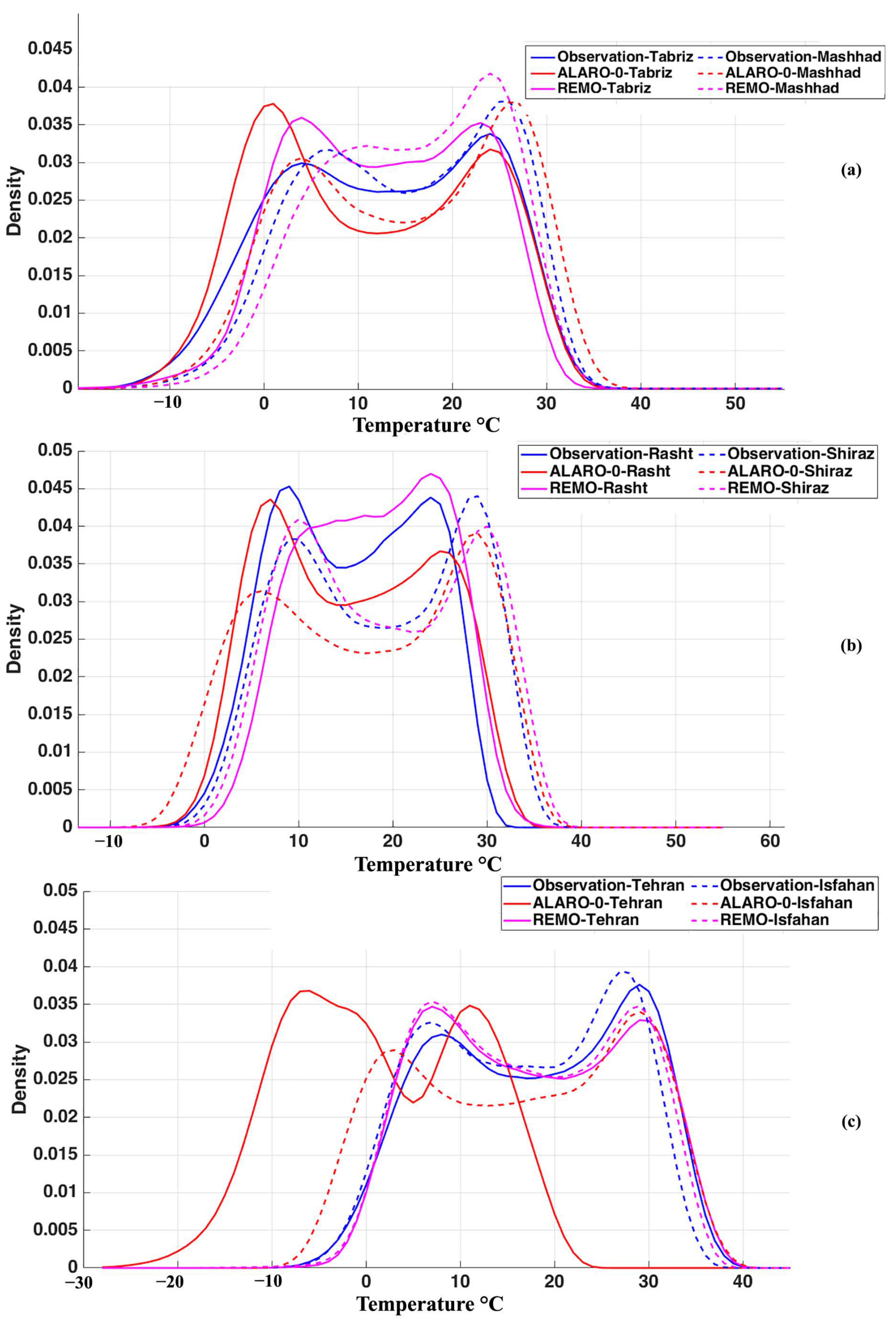
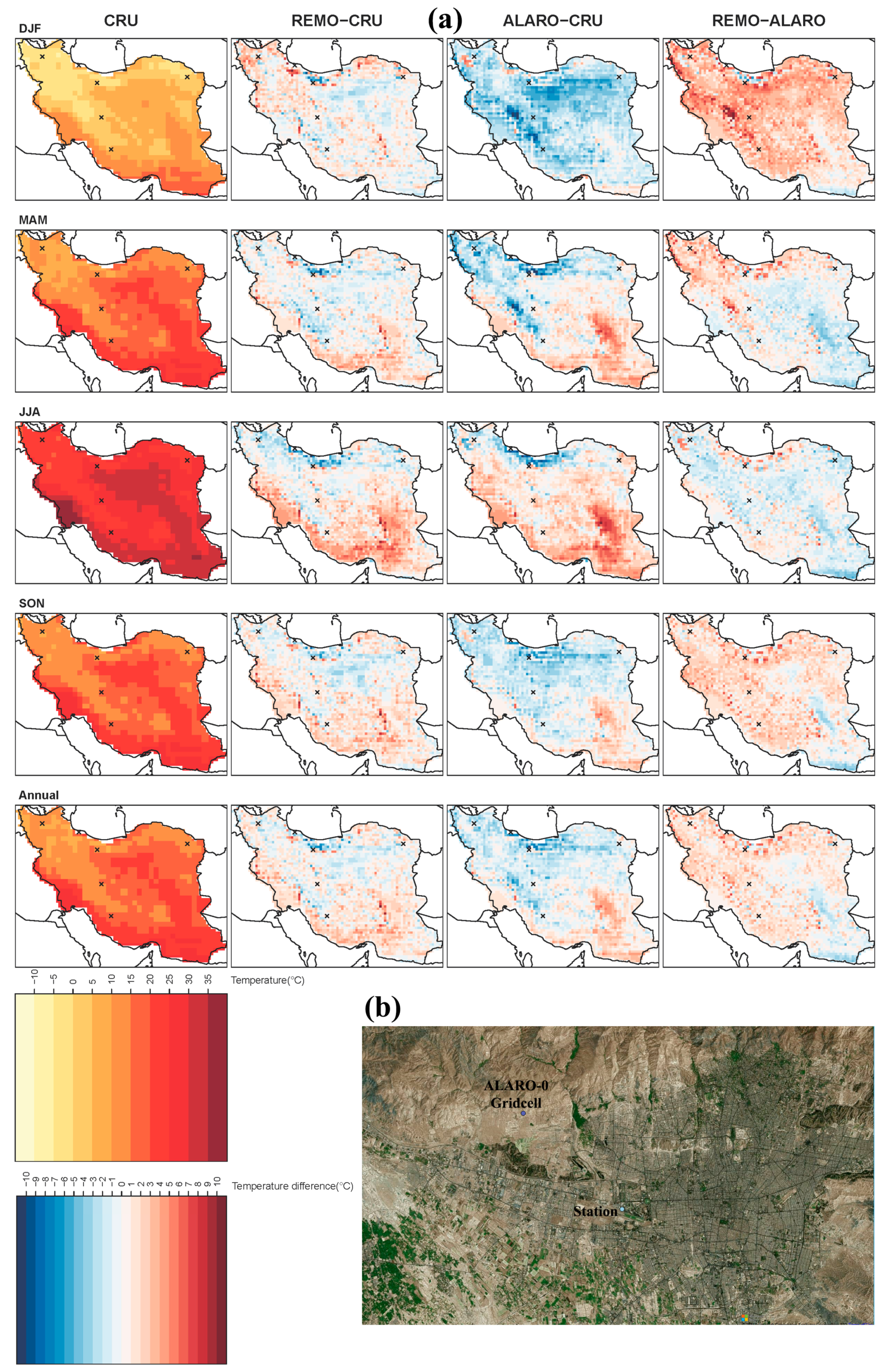
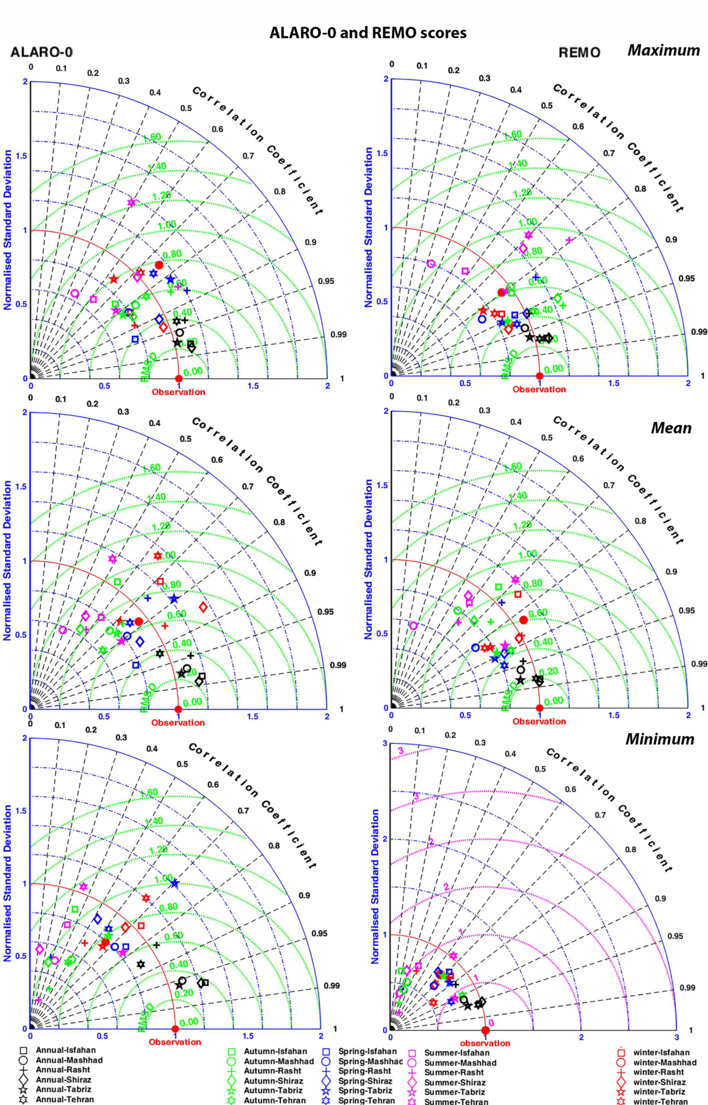
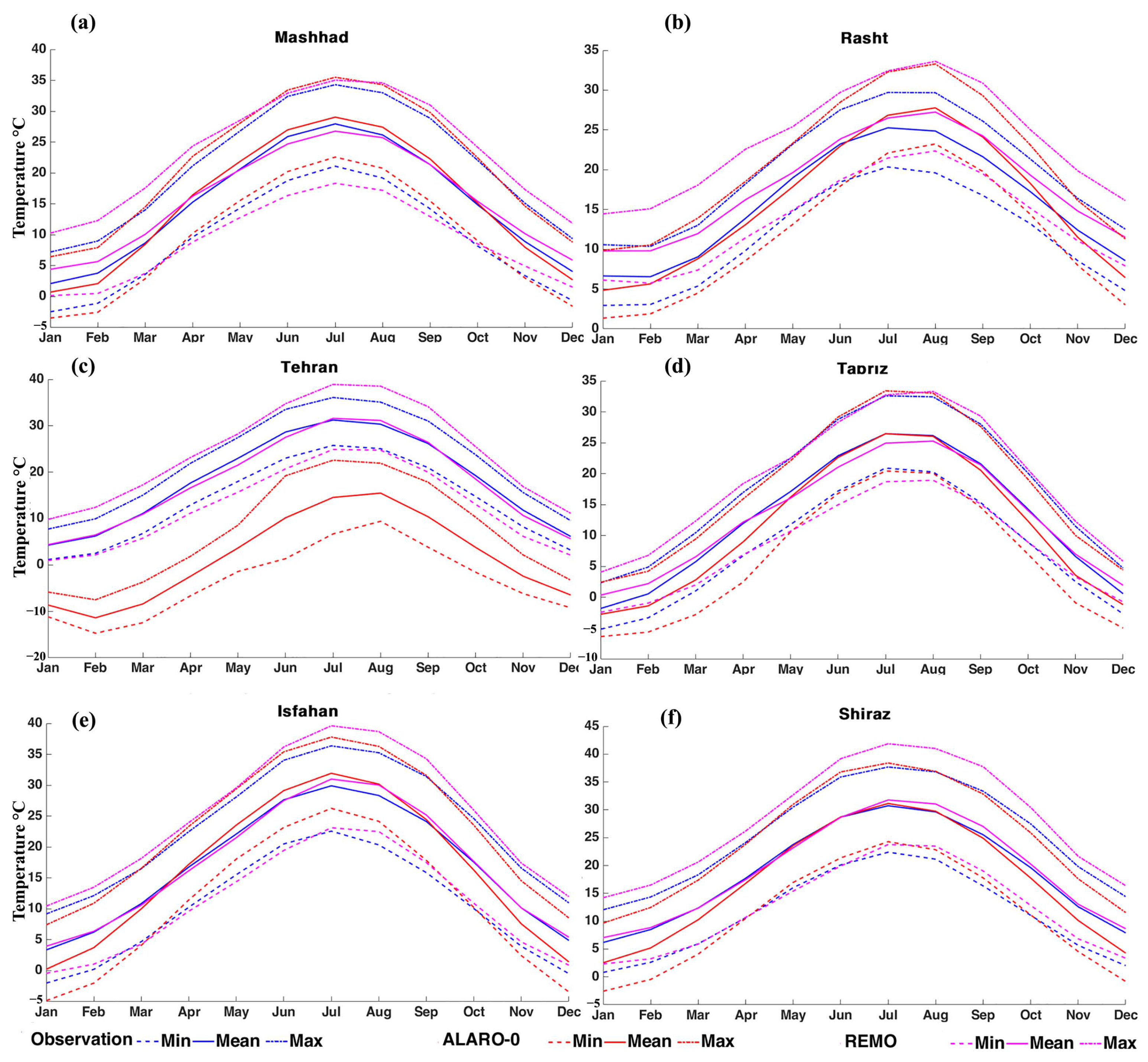
3.1. Temperature
3.1.1. Mean, Minimum, and Maximum Temperature
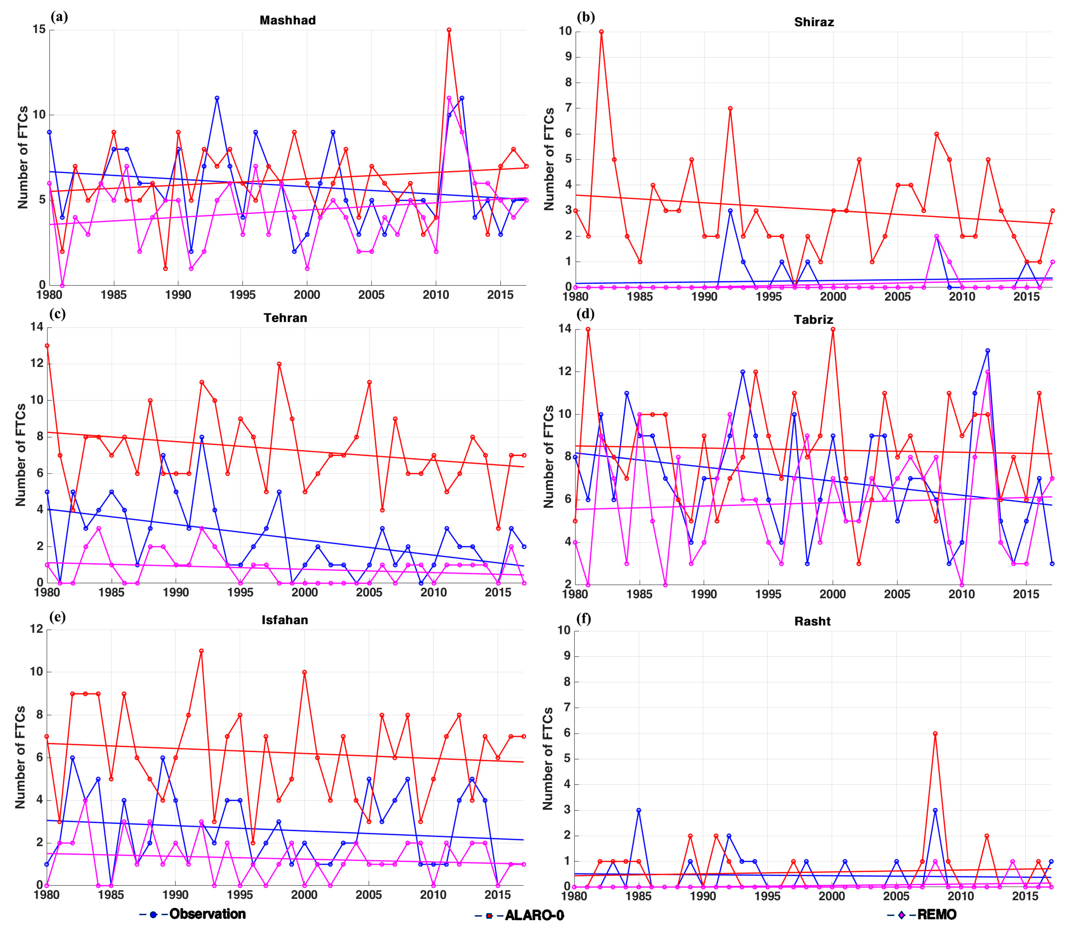
3.1.2. Freeze–Thaw Cycles
3.2. Humidity
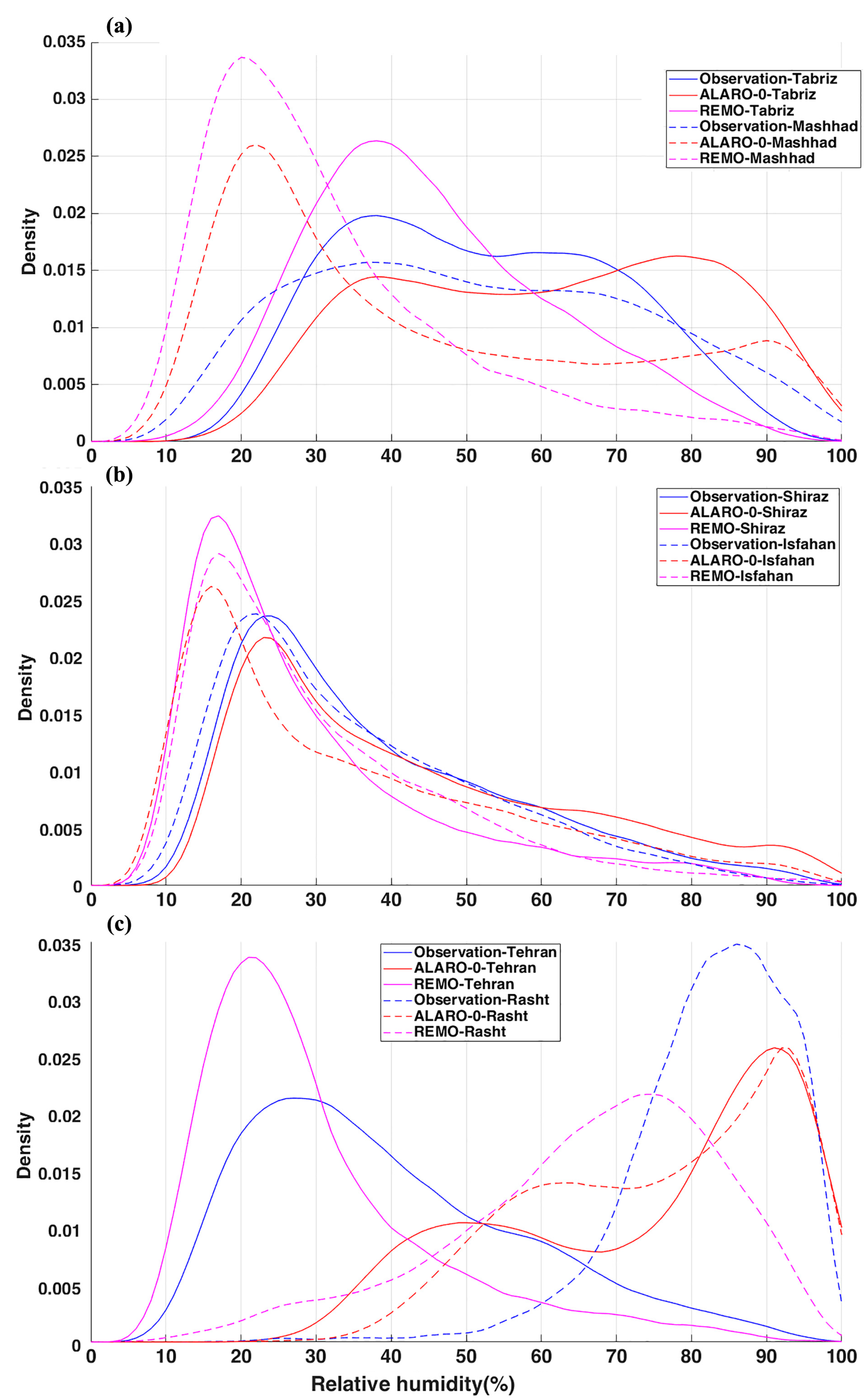
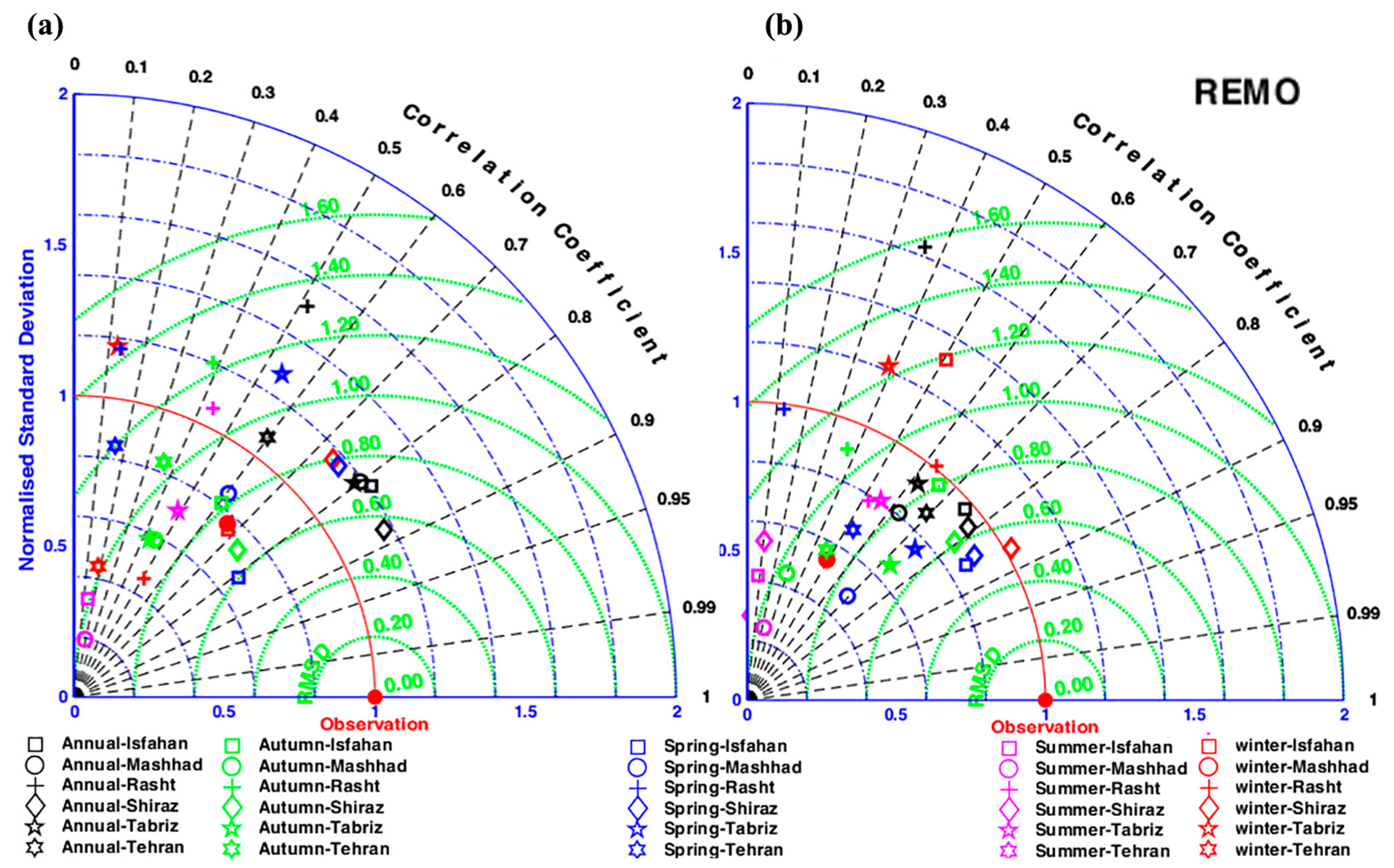
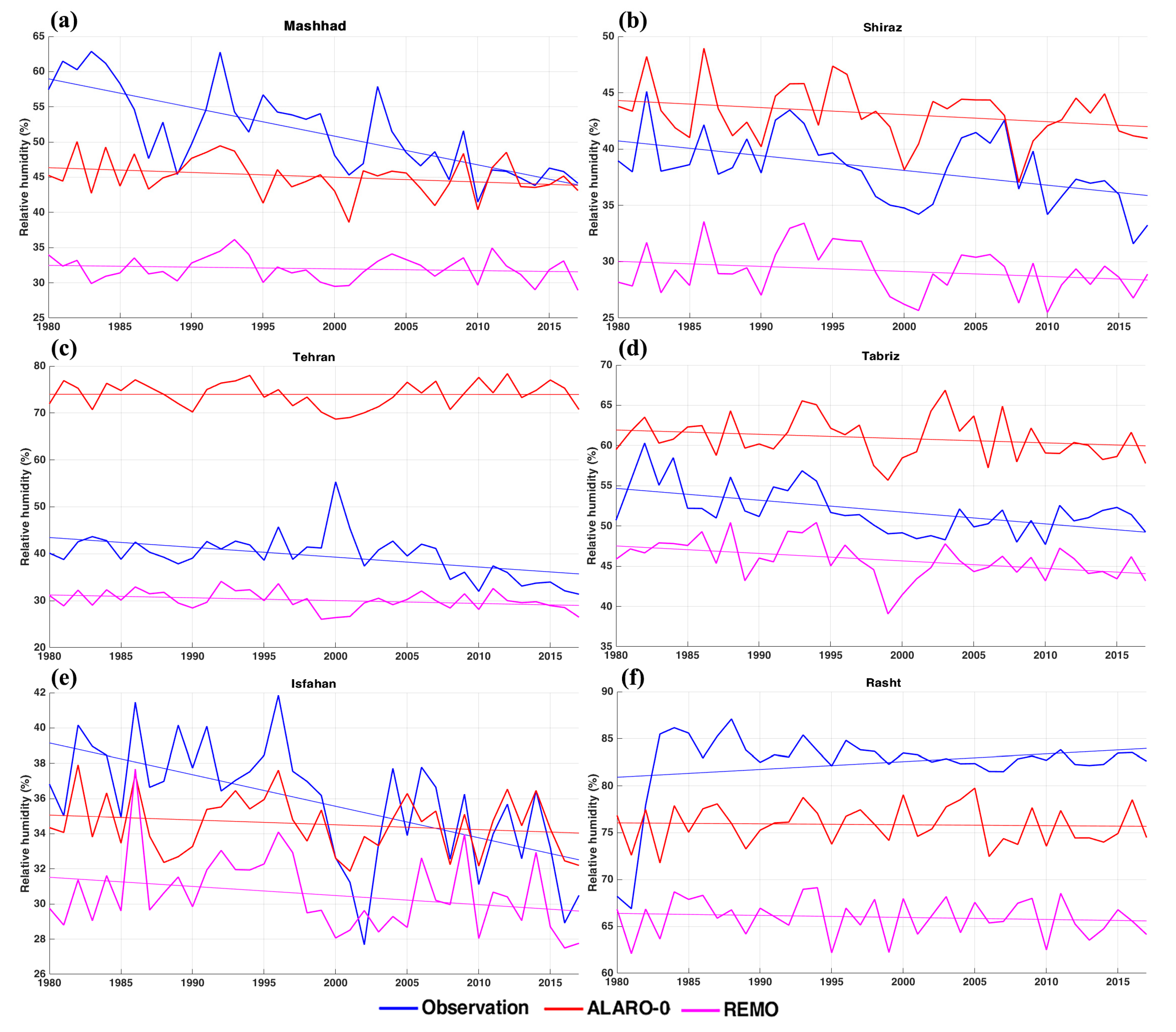
3.2.1. Relative Humidity
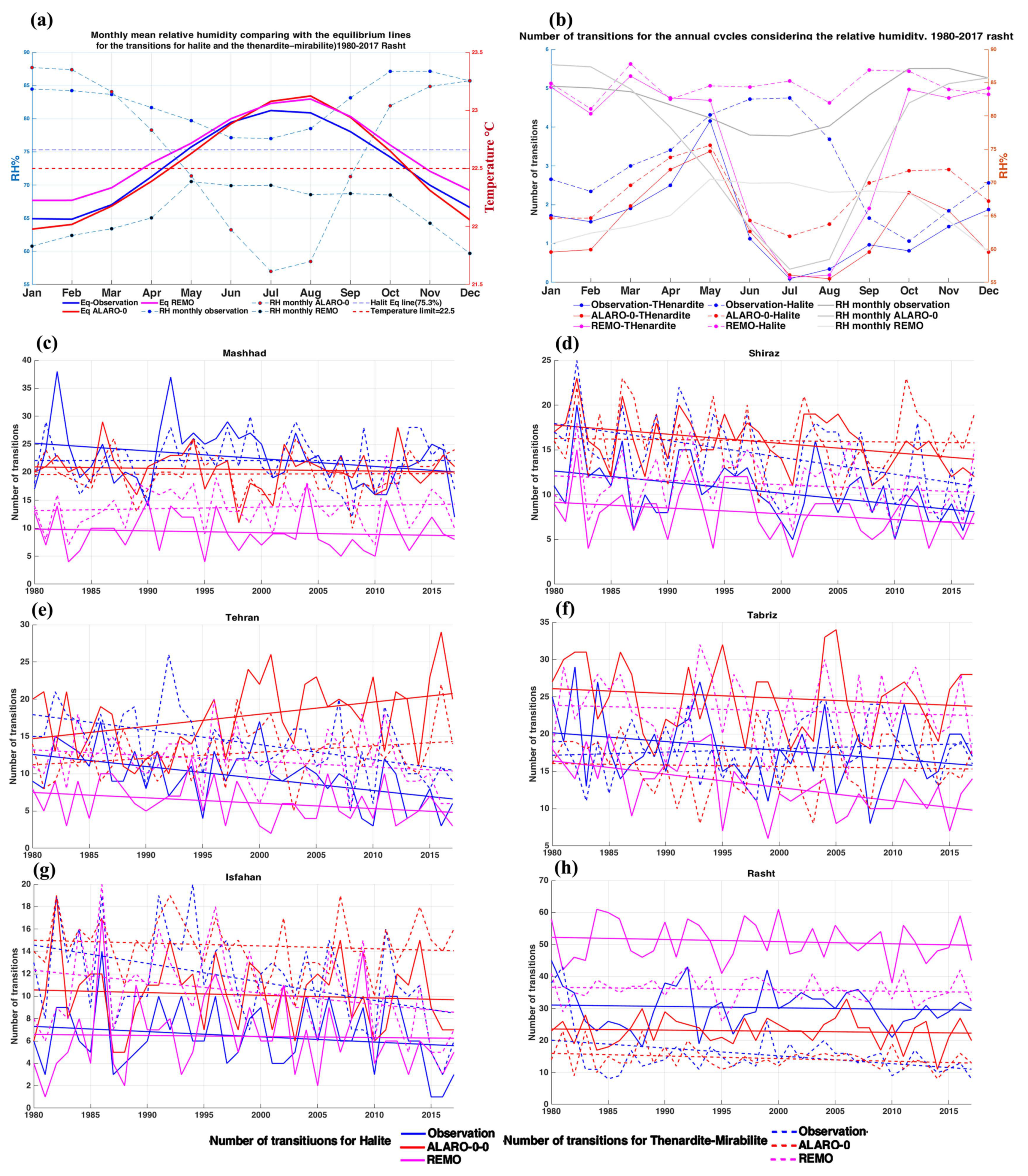
3.2.2. Salt Crystallisation Index
3.3. Wetting and Drying
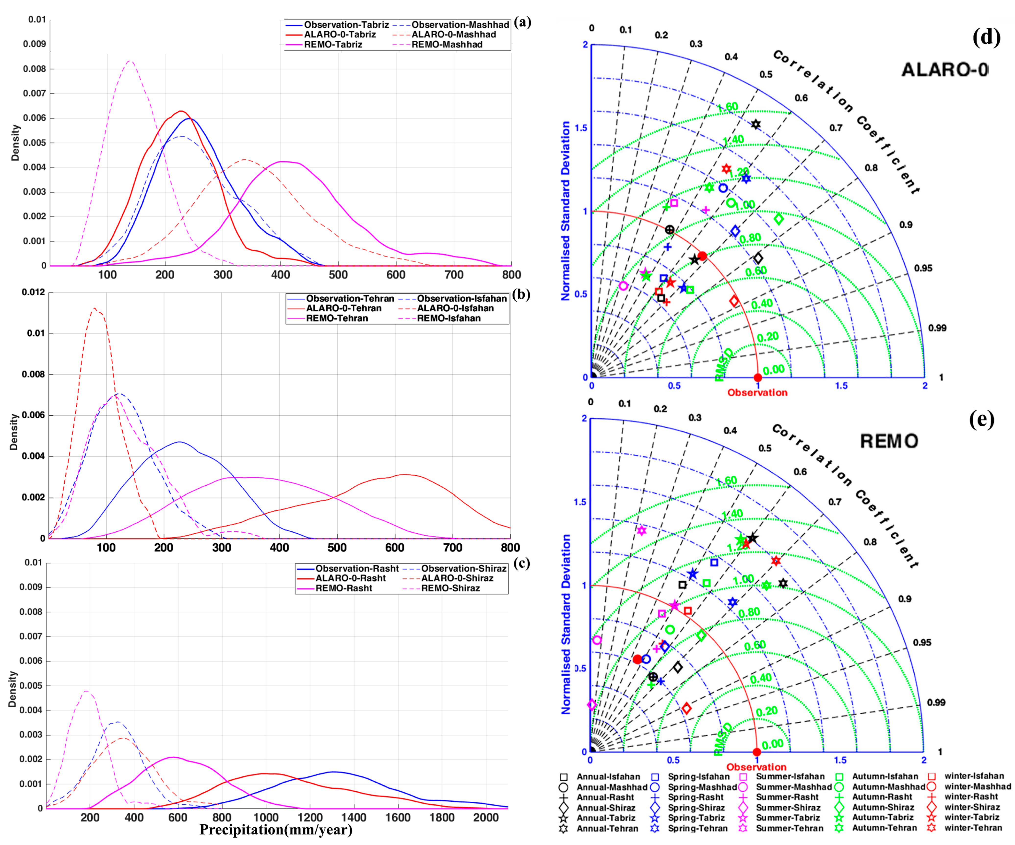
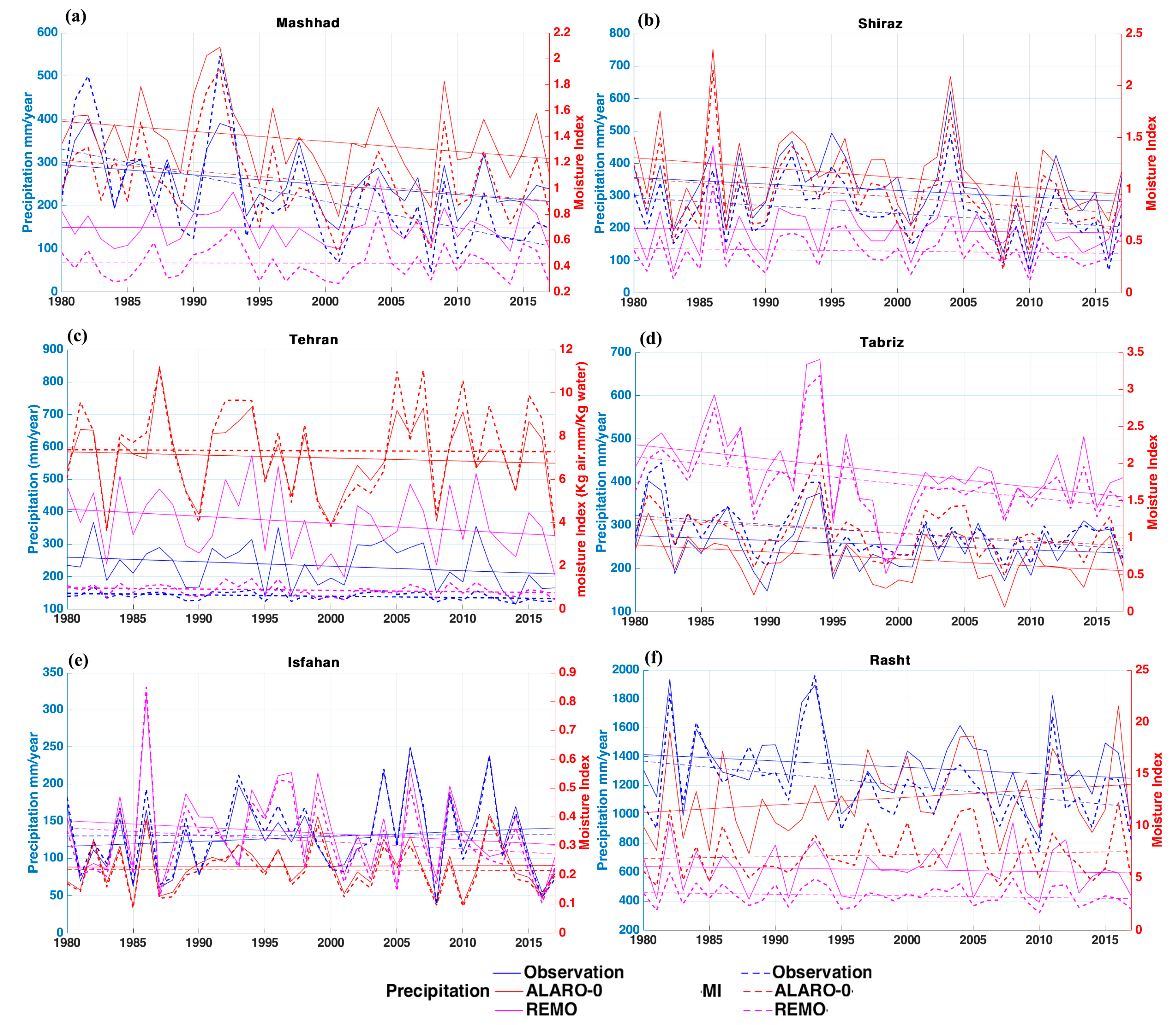
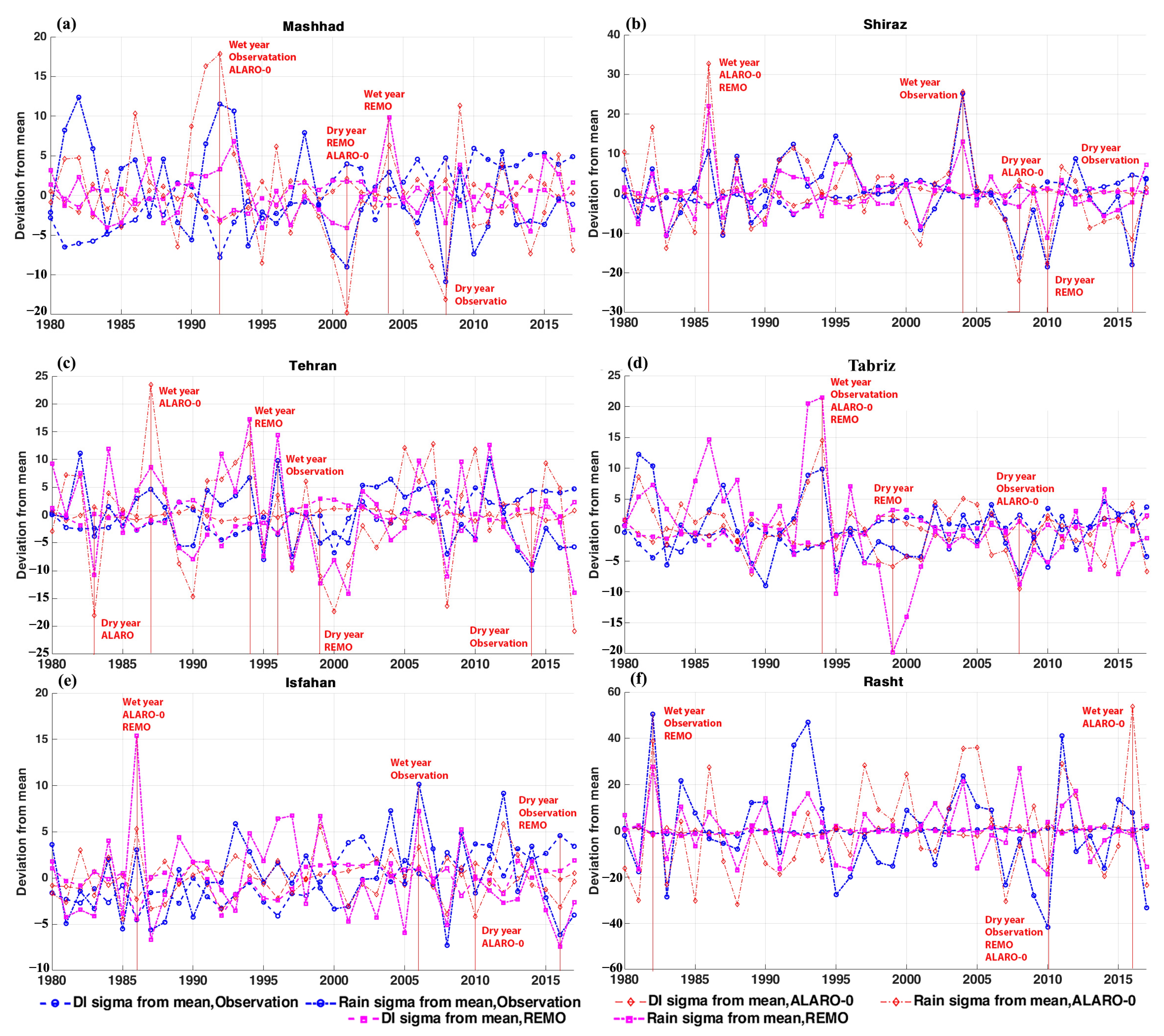
3.3.1. Precipitation
3.3.2. Moisture Index
3.4. Wind Parameters
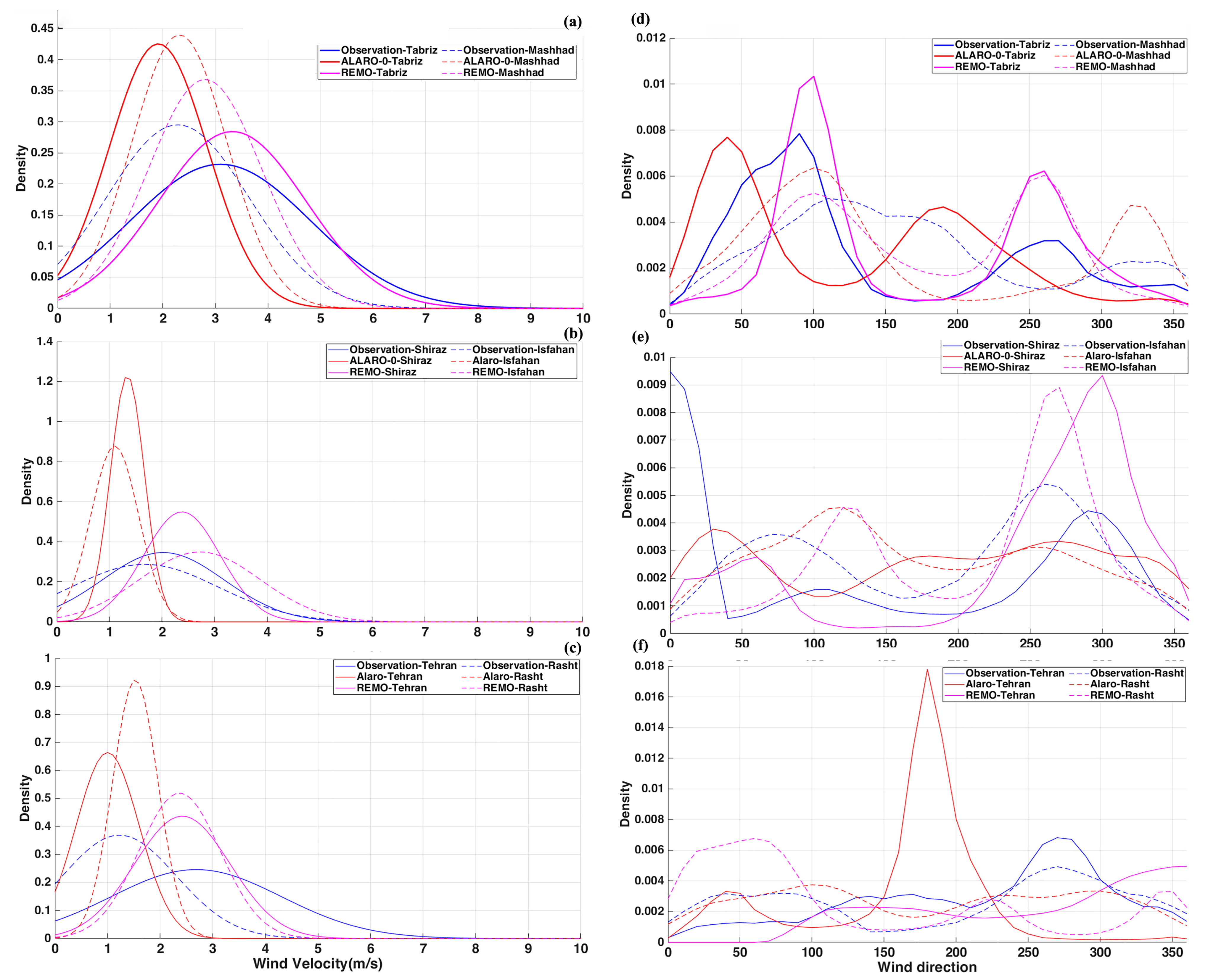
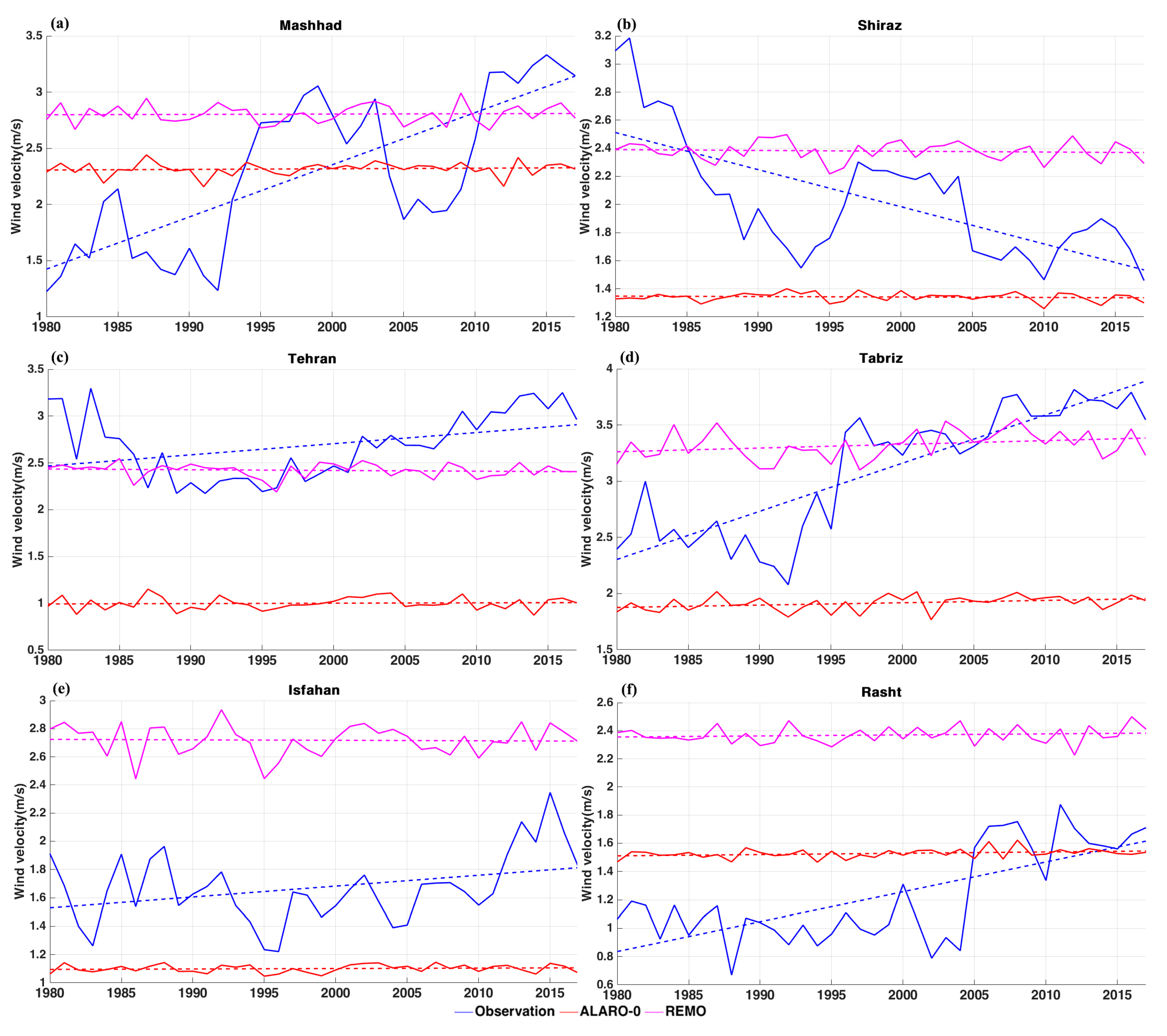
3.4.1. Wind Velocity and Wind Direction
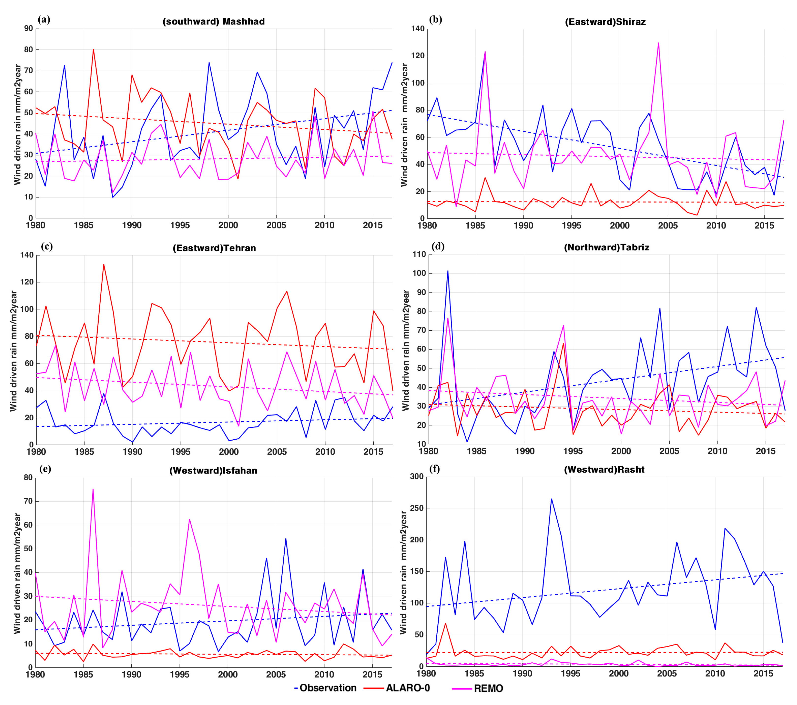
3.4.2. Wind-Driven Rain
4. Conclusions
Supplementary Materials
Author Contributions
Funding
Institutional Review Board Statement
Informed Consent Statement
Data Availability Statement
Acknowledgments
Conflicts of Interest
Nomenclature
| CRU | Climatic research unit |
| FTC | Freeze–thaw cycle |
| MI | Moisture index |
| GCM | General circulation model |
| RCM | Regional climate model |
| RCP | Representative concentration pathway |
| DJF | December, January, February |
| MAM | March, April, May |
| SON | September, October, November |
| JJA | June, July, August |
| RMSD | Root mean square deviation |
| Probability density function | |
| MRY | Moisture reference years |
| HAM | Heat–air–moisture |
| UHI | Urban heat island |
| WDR | Wind-driven rain |
References
- Whatley, C.H. Bought and Sold for English Gold: The Union of 1707; Tuckwell Press: East Linton, UK, 2001. [Google Scholar]
- Beck, H.E.; Zimmermann, N.E.; McVicar, T.R.; Vergopolan, N.; Berg, A.; Wood, E.F. Present and future Köppen-Geiger climate classification maps at km resolution. Sci. Data 2018, 5, 1–12. [Google Scholar] [CrossRef] [PubMed] [Green Version]
- Sabbioni, C.; Brimblecombe, P.; Cassar, M. The Atlas of Climate Change Impact on European Cultural Heritage: Scientific Analysis and Management Strategies; Anthem Press: London, UK, 2010. [Google Scholar]
- Giorgi, F. Climate change hot-spots. Geophys. Res. Lett. 2006, 33, 1–4. [Google Scholar] [CrossRef]
- Ochs, F.; Heidemann, W.; Müller-Steinhagen, H. Effective thermal conductivity of moistened insulation materials as a function of temperature. Int. J. Heat Mass Transf. 2008, 51, 539–552. [Google Scholar] [CrossRef]
- Jerman, M.; Černý, R. Effect of moisture content on heat and moisture transport and storage properties of thermal insulation materials. Energy Build. 2012, 53, 39–46. [Google Scholar] [CrossRef]
- Abdou, A.; Budaiwi, I.M. Comparison of thermal conductivity measurements of building insulation materials under various operating temperatures. J. Build. Phys. 2005, 29, 171–184. [Google Scholar] [CrossRef]
- Dos Santos, W.N. Effect of moisture and porosity on the thermal properties of a conventional refractory concrete. J. Eur. Ceram. Soc. 2003, 23, 745–755. [Google Scholar] [CrossRef]
- Taoukila, D.; Sick, F.; Mimet, A.; Ezbakhe, H.; Ajzoul, T. Moisture content influence on the thermal conductivity and diffusivity of wood-concrete composite. Constr. Build. Mater. 2013, 48, 104–115. [Google Scholar] [CrossRef]
- Jin, H.Q.; Yao, X.L.; Fan, L.W.; Xu, X.; Yu, Z.T. Experimental determination and fractal modeling of the effective thermal conductivity of autoclaved aerated concrete: Effects of moisture content. Int. J. Heat Mass Transf. 2016, 92, 589–602. [Google Scholar] [CrossRef]
- Perez-Bella, J.M.; Dominguez-Hernandez, J.; Cano-Sunen, E.; del Coz-Diaz, J.J.; Rabanal, F.P.A. A correction factor to approximate the design thermal conductivity of building materials. Application to Spanish façades. Energy Build. 2015, 88, 153–164. [Google Scholar] [CrossRef]
- Pérez Bella JMDomínguez Hernández, J.; Cano-Sunen, E.; Alonso-Martinez, M.; Alonso Martínez, M.; del Coz-Diaz, J.J. Detailed territorial estimation of design thermal conductivity for façade materials in North-Eastern Spain. Energy Build. 2015, 102, 266–276. [Google Scholar] [CrossRef]
- Clarke, J.A.; Yaneske, P.P. A rational approach to the harmonisation of the thermal properties of building materials. Build. Environ. 2009, 44, 2046–2055. [Google Scholar] [CrossRef] [Green Version]
- Viitanen, H. Moisture and Bio-Deterioration Risk of Building Materials and Structures. Mass Transf.-Adv. Asp. 2011, 579–594. [Google Scholar] [CrossRef] [Green Version]
- Roberts, M.J.; Camp, J.; Seddon, J.; Vidale, P.L.; Hodges, K.; Vanniere, B.; Mecking, J.; Haarsma, R.; Bellucci, A.; Scoccimarro, E.; et al. Impact of model resolution on tropical cyclone simulation using the HighResMIP-PRIMAVERA multimodel ensemble. J. Clim. 2020, 33, 2557–2583. [Google Scholar] [CrossRef] [Green Version]
- Top, S.; Kotova, L.; De Cruz, L.; Aniskevich, S.; Bobylev, L.; De Troch, R.; Gnatiuk, N.; Gobin, A.; Hamdi, R.; Kriegsmann, A.; et al. Evaluation of regional climate models ALARO-0 and REMO2015 at 0.22° resolution over the CORDEX Central Asia domain. Geosci. Model Dev. 2021, 14, 1267–1293. [Google Scholar] [CrossRef]
- Hawkins, E.; Frame, D.; Harrington, L.; Joshi, M.; King, A.; Rojas, M.; Sutton, R. Observed emergence of the climate change signal: From the familiar to the unknown. Geophys. Res. Lett. 2020, 47, e2019GL086259. [Google Scholar] [CrossRef] [Green Version]
- De Troch, R.; Hamdi, R.; Van de Vyver, H.; Geleyn, J.F.; Termonia, P. Multiscale performance of the ALARO-0 model for simulating extreme summer precipitation climatology in Belgium. J. Clim. 2013, 26, 8895–8915. [Google Scholar] [CrossRef] [Green Version]
- Giot, O.; Termonia, P.; Degrauwe, D.; de Troch, R.; Caluwaerts, S.; Smet, G.; Berckmans, J.; Deckmyn, A.; de Cruz, L.; de Meutter, P.; et al. Validation of the ALARO-0 model within the EURO-CORDEX framework. Geosci. Model Dev. 2016, 9, 1143–1152. [Google Scholar] [CrossRef] [Green Version]
- Remedio, A.R.; Teichmann, C.; Buntemeyer, L.; Sieck, K.; Weber, T.; Rechid, D. Evaluation of New CORDEX simulations using an updated Köppen–Trewartha climate classification. Atmosphere 2019, 10, 726. [Google Scholar] [CrossRef] [Green Version]
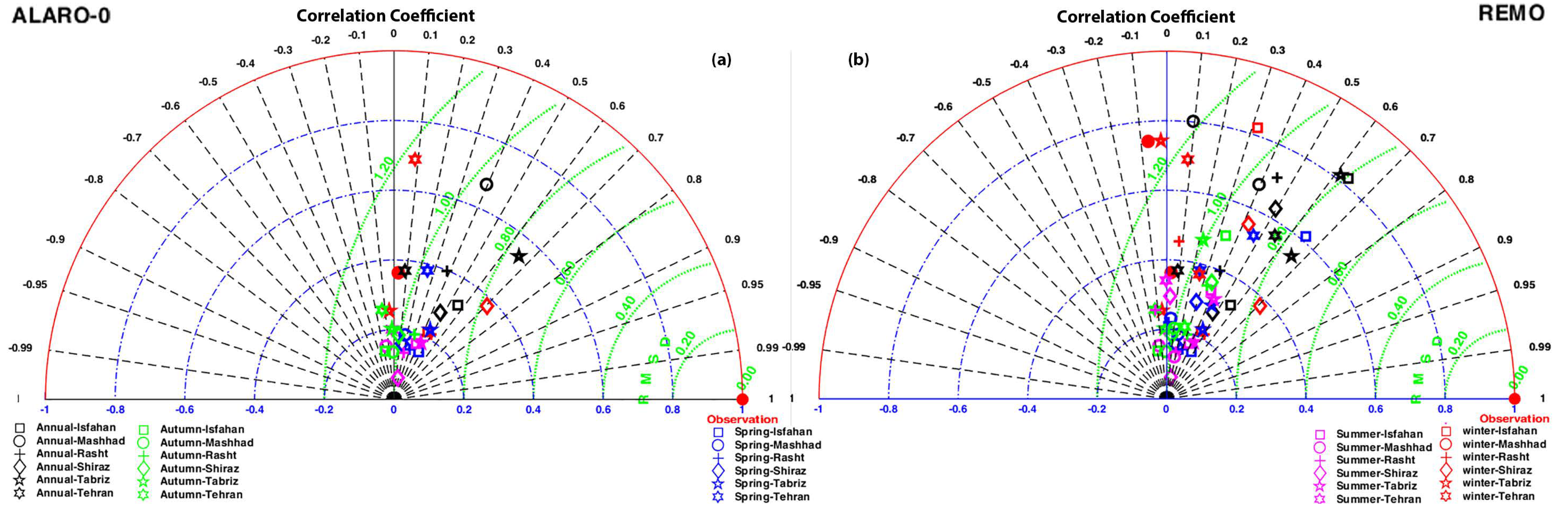
- Taylor, K.E. Summarising multiple aspects of model performance in a single diagram. J. Geophys. Research. Atmos. 2001, 106, 7183–7192. [Google Scholar] [CrossRef]
- Grossi, C.; Brimblecombe, P.; Harris, I. Predicting long term freeze-thaw risks on Europe built heritage and archaeological sites in a changing climate. Sci. Total. Environ. 2007, 377, 273–281. [Google Scholar] [CrossRef]
- Ruiz-Agudo, E.; Mees, F.; Jacobs, P.; Rodriguez-Navarro, C. The role of saline solution properties on porous limestone salt weathering by magnesium and sodium sulfates. Environ. Geol. 2007, 52, 269–281. [Google Scholar] [CrossRef]
- Price, C. The Use of the Sodium Sulphate Crystallisation Test for Determining the Weathering Resistance of Untreated Stone. Deterioration and Protection of Stone Monuments; International Symposium: Paris, France, 1978; Volume 3, p. 10. [Google Scholar]
- Benavente, D.; Brimblecombe, P.; Grossi, C.M. Salt weathering and climate change. In MP. Colombini, L. Tasso, editors. New trends in analytical, environmental and cultural heritage chemistry. Transw. Res. Netw. 2008, 37661, 277–286. [Google Scholar]
- Grossi, C.; Brimblecombe, P.; Menéndez, B.; Benavente, D.; Harris, I.; Déqué, M. Climatology of salt transitions and implications for stone weathering. Sci. Total Environ. 2011, 409, 2577–2585. [Google Scholar] [CrossRef]
- Cornick, S.; Djebbar, R.; Dalgliesh, W. Selecting moisture reference years using a Moisture Index approach. Build. Environ. 2003, 38, 1367–1379. [Google Scholar] [CrossRef]
- ISO, E. Hygrothermal performance of buildings-calculation and presentation of climatic data-Part 3: Calculation of a driving rain index for vertical surfaces from hourly wind and rain data. BS EN ISO 2009, 2009, 15927-3. [Google Scholar]
- Oke, T. City Size and the Urban Heat Island. Atmos. Environ. 1973, 7, 769–779. [Google Scholar] [CrossRef]
- Hedayatnia, H.; Steeman, M.; Van Den Bossche, N. Conservation of heritage buildings in Mashhad: On the impact of climate change and the urban heat island effect. ICMB21 2021. [Google Scholar] [CrossRef]
- Liu, W.; You, H.; Dou, J. Erratum to Urban-rural humidity and temperature differences in the Beijing area. Theor. Appl. Climatol. 2010, 96, 201–207. [Google Scholar] [CrossRef]
- Wang, Z.; Song, J.; Chan, P.W.; Li, Y. The urban moisture island phenomenon and its mechanisms in a high-rise high-density city. Int. J. Climatol. 2020, 41, E150–E170. [Google Scholar] [CrossRef]


| Location | Tehran | Mashhad | Shiraz | Tabriz | Rasht | Isfahan |
|---|---|---|---|---|---|---|
| Coordinates | 35.41° N/51.19° E | 36.2° N/52.6° E | 29.6° N/52.6° E | 38.1° N/46.2° E | 37.3° N/49.6° E | 32.5° N/51.7° E |
| Orographic features | Alborz Mountains to the north and central desert to the south | Valley of Kashafrud River, between two mountain ranges of Binalood and Hezar Masjed | Shiraz plain surrounded by mountain ranges with an average height of 2000 m | Located between Eynali and Sahand mountains in a fertile area | City on Caspian Sea coast | Situated at foothills of Zagros mountain range |
| Altitude (m) | 1191 | 999.2 | 1488 | 1361 | −8.6 | 1550.4 |
| ALARO-0 altitude (m) | 1485.45 | 1343 | 1749 | 1682 | 16.7 | 1705 |
| REMO altitude (m) | 1109.7 | 1087 | 1723 | 1567 | −1 | 1683 |
| Climate | Bsk/Csa/Dsa | Bsk | BSh/Bsk | Dsa | Csa | BSk |
| Mean Tmin (°C) | 10.5 | 7.3 | 9.2 | 7.2 | 11.1 | 9.4 |
| Mean Tmax (°C) | 20.4 | 21.2 | 25.6 | 18.2 | 20.5 | 23.1 |
| Annual precipitation (mm/year) | 429.2 | 251.5 | 305.6 | 318.8 | 1255.5 | 114.3 |
| Reference Parameters | Air Temperature | Precipitation | Relative Humidity | Wind Velocity | Wind Direction |
|---|---|---|---|---|---|
| Temporal resolution observations | 3-h 2 m | 6-h | 3-h | 3-h at 10 m | 3-h at 10 m |
| Temporal resolution model data | 1-h 2 m | 1-h | 3-h | 1-h at 10 m | 6-h at 10 m |
| Observations | ALARO-0 | REMO | |||||||
|---|---|---|---|---|---|---|---|---|---|
| Mean of FTCs | Trend Slope | Normalised FTC | Mean of FTCs | Trend Slope | Normalised FTC | Mean of FTCs | Trend Slope | Normalised FTC | |
| Isfahan | 2.6 | Decremental | 1 | 6.2 | Decremental | 2.4 | 1.3 | Decremental | 0.50 |
| Mashhad | 5.86 | Decremental | 1 | 6.21 | Incremental | 1.06 | 4.4 | Incremental | 0.75 |
| Rasht | 0.45 | Decremental | 1 | 0.58 | Incremental | 1.3 | 0.5 | Incremental | 1.1 |
| Shiraz | 0.26 | Decremental | 1 | 3 | Incremental | 11.5 | 0.1 | Decremental | 0.40 |
| Tabriz | 7 | Decremental | 1 | 8.3 | Decremental | 1.2 | 5.8 | Incremental | 0.80 |
| Tehran | 2.5 | Decremental | 1 | 7.3 | Decremental | 2.9 | 0.8 | Decremental | 0.32 |
| Observation | ALARO-0 | REMO | ||||||||||
|---|---|---|---|---|---|---|---|---|---|---|---|---|
| Halite | T-M | Halite | T-M | Halite | T-M | |||||||
| N | T | N | T | N | T | N | T | N | T | N | T | |
| Isfahan | 6.4 | −0.05 | 11.5 | −0.16 | 10 | −0.02 | 14.5 | −0.03 | 6.4 | −0.01 | 10.4 | −0.1 |
| Mashhad | 22.6 | −0.14 | 22.1 | 0.0003 | 21 | −0.03 | 19.7 | 0.004 | 9.3 | −0.03 | 13.7 | 0.03 |
| Rasht | 30.32 | −0.04 | 15.6 | −0.24 | 23 | −0.04 | 14.5 | −0.08 | 51 | −0.07 | 36 | −0.04 |
| Shiraz | 10.4 | −0.12 | 16 | −0.19 | 16 | −0.1 | 11.2 | −0.014 | 14.4 | −0.06 | 8 | −0.05 |
| Tabriz | 18 | −0.12 | 18 | 0.04 | 25 | −0.06 | 15.7 | −0.02 | 13.1 | −0.18 | 23.2 | −0.04 |
| Tehran | 9.6 | −0.16 | 14.2 | −0.2 | 18 | 0.16 | 12.8 | 0.08 | 6.2 | −0.07 | 11.2 | −0.08 |
| Observations | ALARO-0 | REMO | ||||
|---|---|---|---|---|---|---|
| MI | MI | MI | ||||
| MI Mean | Slope | MI Mean | Slope | MI Mean | Slope | |
| Isfahan | 0.34 | −0.001 | 0.22 | −0.001 | 0.34 | −0.006 |
| Mashhad | 0.85 | −0.02 | 1.05 | −0.01 | 0.43 | −0.001 |
| Rasht | 13.75 | −0.15 | 7.3 | 0.0001 | 3.3 | −0.02 |
| Shiraz | 0.8 | −0.01 | 0.94 | −0.02 | 0.42 | −0.005 |
| Tabriz | 1.03 | −0.008 | 1.04 | −0.01 | 1.7 | −0.02 |
| Tehran | 0.6 | −0.008 | 7.35 | 0.001 | 0.86 | −0.007 |
| Observation | ALARO-0 | REMO | ||||
|---|---|---|---|---|---|---|
| Wind-Driven Rain | Wind-Driven Rain | Wind-Driven Rain | ||||
| WDR | Slope | WDR | Slope | WDR | Slope | |
| Isfahan | 18.6 | −0.16 | 7.65 | 0.05 | 28.15 | −0.48 |
| Mashhad | 35.5 | 0.91 | 81.5 | −0.8 | 35.5 | 0.2 |
| Rasht | 285.4 | 0.53 | 88.12 | 0.32 | 37.4 | 0.3 |
| Shiraz | 26.8 | −1.05 | 13 | −0.1 | 50 | −0.8 |
| Tabriz | 51.3 | −1.05 | 35 | −0.1 | 65.5 | 1.3 |
| Tehran | 16.7 | 0.17 | 75.8 | −0.28 | 43.4 | −0.7 |
Publisher’s Note: MDPI stays neutral with regard to jurisdictional claims in published maps and institutional affiliations. |
© 2021 by the authors. Licensee MDPI, Basel, Switzerland. This article is an open access article distributed under the terms and conditions of the Creative Commons Attribution (CC BY) license (https://creativecommons.org/licenses/by/4.0/).
Share and Cite
Hedayatnia, H.; Top, S.; Caluwaerts, S.; Kotova, L.; Steeman, M.; Van Den Bossche, N. Evaluation of ALARO-0 and REMO Regional Climate Models over Iran Focusing on Building Material Degradation Criteria. Buildings 2021, 11, 376. https://doi.org/10.3390/buildings11080376
Hedayatnia H, Top S, Caluwaerts S, Kotova L, Steeman M, Van Den Bossche N. Evaluation of ALARO-0 and REMO Regional Climate Models over Iran Focusing on Building Material Degradation Criteria. Buildings. 2021; 11(8):376. https://doi.org/10.3390/buildings11080376
Chicago/Turabian StyleHedayatnia, Hamed, Sara Top, Steven Caluwaerts, Lola Kotova, Marijke Steeman, and Nathan Van Den Bossche. 2021. "Evaluation of ALARO-0 and REMO Regional Climate Models over Iran Focusing on Building Material Degradation Criteria" Buildings 11, no. 8: 376. https://doi.org/10.3390/buildings11080376