Rotation-Free Based Numerical Model for Nonlinear Analysis of Thin Shells

Abstract

This paper presents a computationally efficient numerical model for the analysis of thin shells based on rotation-free triangular finite elements. The geometry of the structure in the vicinity of the observed triangular element is approximated through a controlled domain consisting of nodes of the observed finite element and nodes of three adjacent finite elements between which a second-order spatial polynomial is defined. The model considers large displacements, large rotations, small strains, and material and geometrical nonlinearity. Material nonlinearity is implemented by considering the von Mises yield criterion and the Levi–Mises flow rule. The model uses an explicit time integration scheme to integrate motion equations but an implicit radial returning algorithm to compute the plastic strain at the end of each time step. The presented numerical model has been embedded in the program Y based on the finite–discrete element method and tested on simple examples. The advantage of the presented numerical model is displayed through a series of analyses where the obtained results are compared with other results presented in the literature.

1. Introduction

Shells, as structural elements, have been frequently applied in civil, automotive, naval, and aerospace engineering. The finite element (FE) method [1,2,3,4,5] is the principal analytical tool for shell structures. The analysis of shells by the FE method has a long tradition, going back to the 1970s [6], which is almost as long as the history of the method itself. Most numerical models for the analysis of shells are founded on planar FEs with six or five degrees of freedom (DOF) per node (three rotations and three translations, or two rotations and three translations) [7,8]. Alternatively, some researchers [9,10] used the approach in which rotations are not represented by normal (pseudo) vectors but by the components of polar (proper) vectors, resulting in the symmetry of the tangent stiffness matrix. Symmetric element tangent stiffness matrices lead to computational efficiency and major computer storage saving. In the last forty years, few numerical models dealing with rotation-free formulations [11,12,13] have emerged, in which only three translations at each node are retained as the degrees of freedom. The advantage of such numerical models is that they significantly simplify the problem and are computationally highly efficient compared to these numerical models involving rotation. In fact, rotation-free numerical models can significantly reduce the number of degrees of freedom in solving particular problems. In addition, rotation-free numerical models can avoid problems with ill-conditioned stiffness matrices caused by the introduction of rotational DOF, in solving systems of equations with many unknowns. Moreover, rotation-free numerical models, in combination with explicit integration schemes for transient dynamics, are suitable for parallel programming, which can be performed at the control domain level.

Probably the first numerical formulation, which belongs to the group of rotation-free numerical models, was proposed by Phaal and Calladine [14,15]. This numerical model is based on the concept that the alteration of curvature at the examined finite element is related to the coordinates of three neighbouring FE nodes. In fact, the shell geometry in the surroundings of the examined FE is approximated by a second-order spatial polynomial that passes through the nodes of the examined FE and the nodes of the three neighbouring FEs. Finally, the alteration of curvature of the shell itself is related to the alteration of curvature of the spatial second-order polynomial. Nonetheless, the numerical model suggested by Phaal and Calladine was limited for the analyses of elastic problems with small displacement.

Shortly after Phaal and Calladine published the paper [14,15], Oñate and Cervera proposed a numerical model for plates based on rotation-free formulation [16] followed by a series of numerical models for shells based on rotation-free formulations [17,18,19,20], including orthotropic behaviour [20] and large strain plasticity [18]. Proposed numerical algorithms are based on the discretisation of plates and shells into three-noded triangles, the linear FE approximation of the displacement field within each triangle, and the finite-volume-type approach for computing the curvature and bending moment fields within the appropriate non-overlapping control domains using the mixed Hu–Washizu functional formulation.

Another rotation-free shell finite element numerical model was proposed by Linhardt et al. [21], who used isoparametric displacement elements to describe membrane strains, while the calculation of curvature for the determination of bending strains was based on the geometry of the surrounding elements.

Stolarski et al. [22] also presented a numerical formulation—based on rotation-free formulation—for the analysis of thin shells with large deflections. This approach combines the formulations of previous contributors to the subject matter, particularly that of Phaal and Calladine for plates, with the algorithmic adjustments required to model shells and large deformations. However, the model is restricted to the linear-elastic material behaviour.

Uzelac et al. [23,24] presented the numerical model 4-TRIELS for the geometric nonlinear analysis of thin shells defined with rotation-free triangular FEs with three nodes. Curvature within an observed FE in the proposed numerical formulation is calculated by considering the neighbouring finite element nodes between which a spatial quadratic polynomial is laid. Pursuant to the alteration of the curvature of the spatial quadratic polynomial, the bending and twisting moments, and, finally, the nodal forces on the corresponding three-noded finite element, were determined. The 4-TRIELS numerical model has proven to be promising in the analysis of thin shells considering linear-elastic material behaviour with hyperelastic constitutive law.

Within this paper, a 4-TRINONL numerical model for the analysis of thin shells, including material and geometrical nonlinearity, is presented. Similar to the 4-TRIELS numerical model, the proposed numerical formulation is also based on the control domain consisting of one observed and three adjacent triangular finite elements over which a second-order spatial polynomial is laid. However, in the presented numerical model, integration points for monitoring strain and stress state along the shell thickness were introduced. Strains in integration points were calculated based on the alteration of the curvature of the spatial square polynomial, while the normal forces and the bending and twisting moments were obtained through the numerical integration of stress by shell thickness. Material nonlinearity was taken into account considering the hypo-elastoplastic material model with von Mises yield criterion and Levi–Mises flow rule. Proposed numerical formulations use an explicit time integration algorithm for transient dynamics, but an implicit radial returning algorithm for computing the plastic strain at the end of each time step. Proposed numerical algorithms were implemented in program Y based on the combined finite–discrete element method (FDEM) [25,26,27,28,29]. The adopted material model is suitable for the analysis of metal structures [30]; however, the proposed numerical model can be easily upgraded with any other material model that would be suitable for the analysis of concrete, reinforced concrete, or any other structures.

The paper is structured as follows. The second section describes the discretisation of the shell structure within the proposed numerical model and the procedure for the calculation of strain at the Gaussian points. This section provides a detailed description of the implemented material model, including the yield criterion and flow rule. It also includes the presentation of normal and bending stresses via nodal forces. The third section presents the numerical examples which demonstrate the validity and the fields of application of the presented model, while the fourth section provides the final comments related to the model development and the guidelines for further research.

2. The Proposed Numerical Formulation

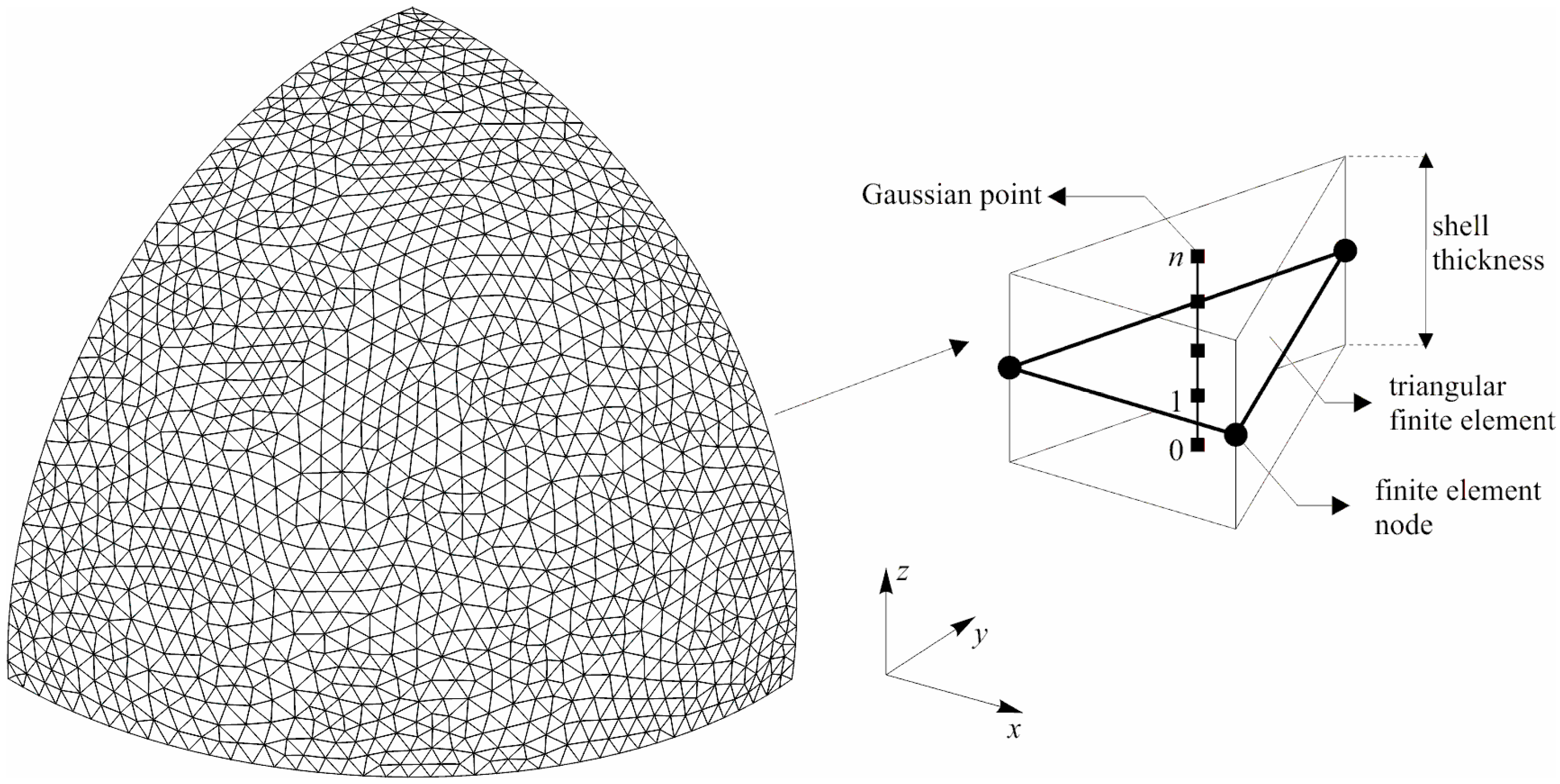
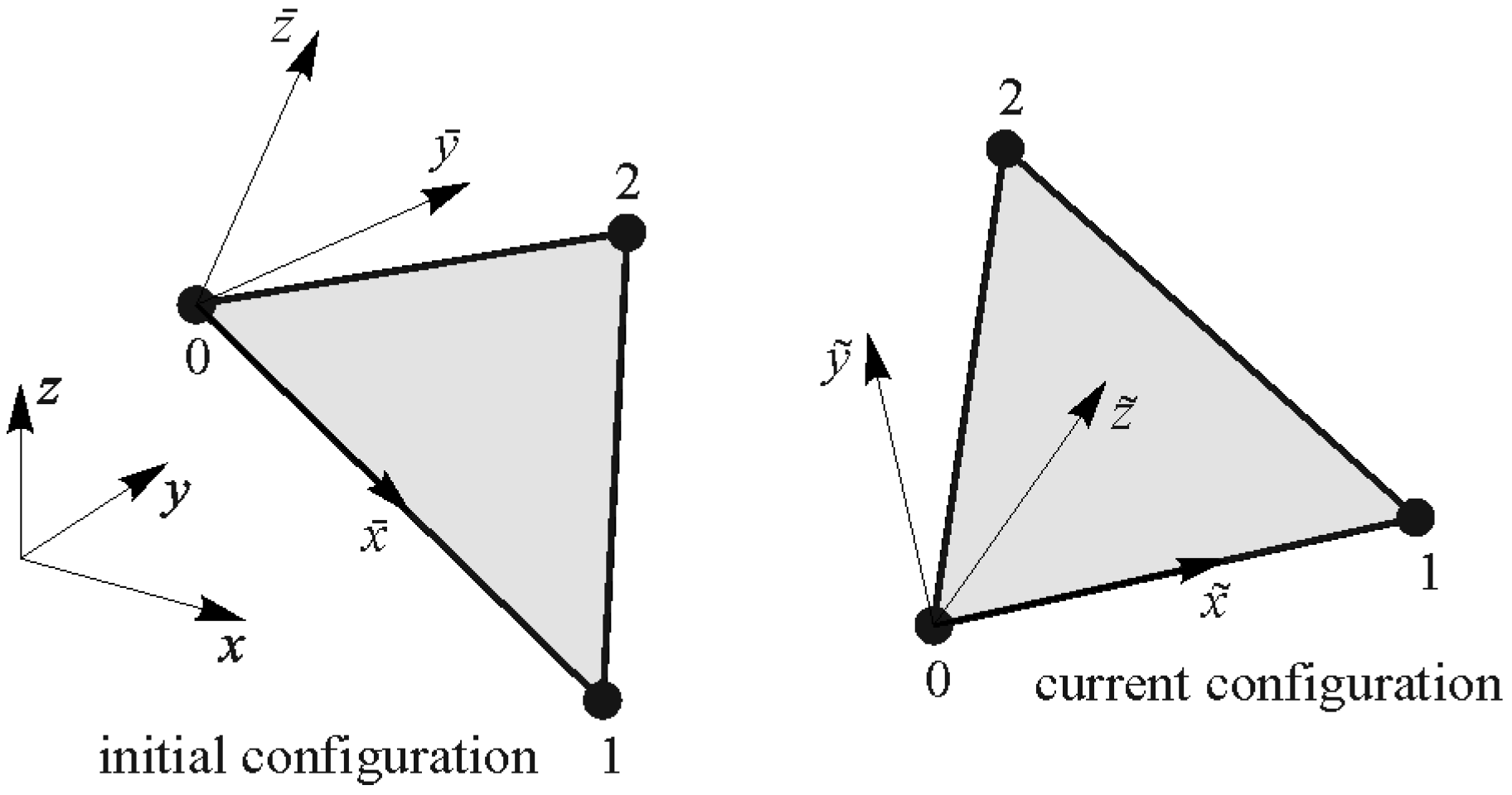
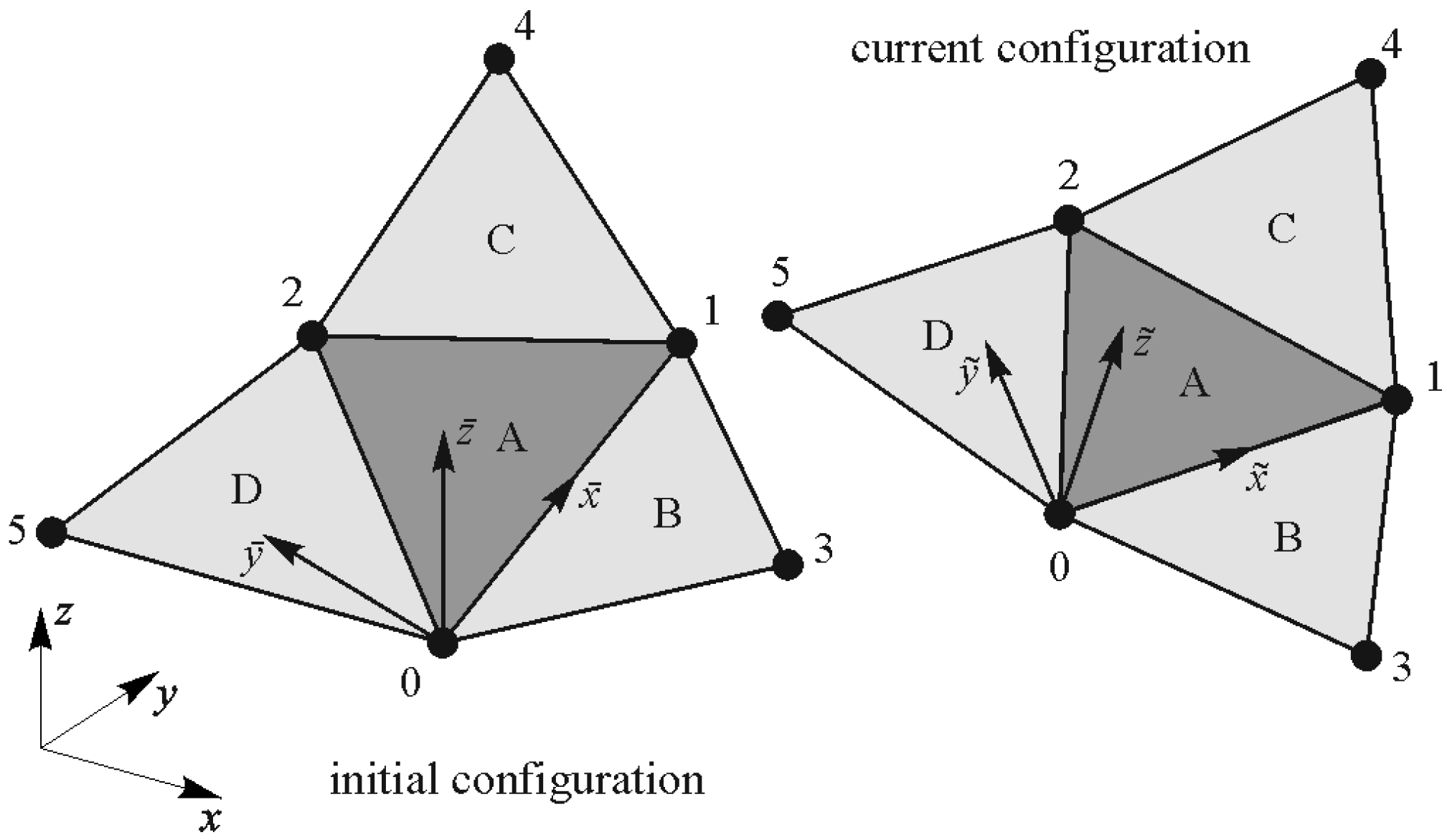
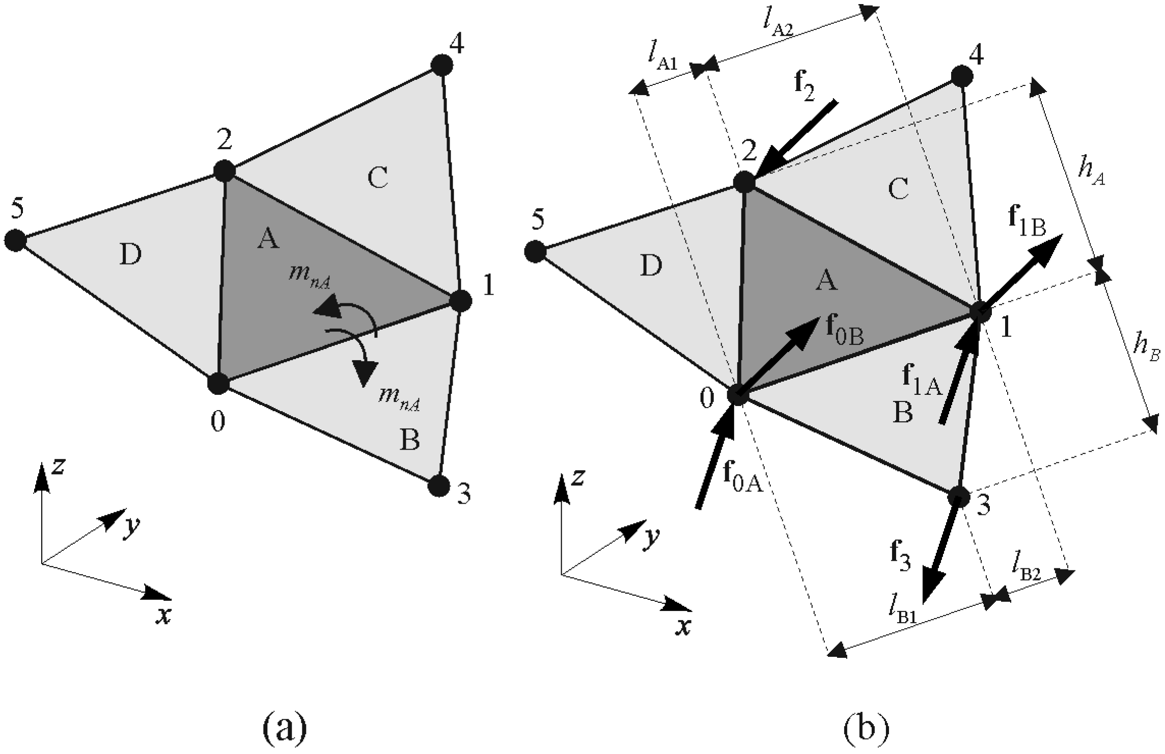
This section presents detailed information regarding the proposed numerical formulation. The discretisation of the structure, detailed information related to the material model, membrane and transverse carrying mechanism, and the presentation of internal forces are provided below.

2.1. Discretisation

In the presented formulation, shells are discretised with triangular FEs, as shown in Figure 1. Perpendicular to the plane of the observed finite element, n numerical integration points were introduced in order to determine stress and strains by shell thickness. Masses are lumped into the finite element nodes, while the transient dynamics for each degree of freedom is solved by using an explicit scheme.

2.2. Calculation of Strain at Gaussian Points

Strains in the middle surface of the subjected FE are determined on the basis of the already defined coordinates of the FE nodes. At the beginning of the calculation, at time t = 0, all nodes have their initial coordinates. Due to the activity of the load, the nodes change their position in space and time, and, at the observed time t = t_i, all nodes have their current coordinates. For the purposes of simplicity and computational efficiency, in addition to the global coordinate system, a local coordinate system is introduced, which is fixed to node 0 of the observed triangle as it is presented in Figure 2. Coordinates (x, y, z) refer to the global coordinate system, coordinates ($\stackrel{-}{x}$, $\stackrel{-}{y}$, $\stackrel{-}{z}$) refer to the initial local coordinate system, and coordinates ($\tilde{x}$, $\tilde{y}$, $\tilde{z}$) refer to the current local coordinate system.

A local coordinate system is introduced to enhance CPU efficiency while preserving a consistent multiplicative decomposition. The global coordinates of each FE node are mapped onto the local coordinate system. The deformation gradient F is then obtained as [25]:

$$F=\left[\begin{array}{cc}{\tilde{x}}_1-{\tilde{x}}_0& {\tilde{x}}_2-{\tilde{x}}_0\\ {\tilde{y}}_1-{\tilde{y}}_0& {\tilde{y}}_2-{\tilde{y}}_0\end{array}\right] {\left[\begin{array}{cc}{\overline{x}}_1-{\overline{x}}_0& {\overline{x}}_2-{\overline{x}}_0\\ {\overline{y}}_1-{\overline{y}}_0& {\overline{y}}_2-{\overline{y}}_0\end{array}\right]}^{-1}$$

(1)

Since the first node of the FE is also the origin of the local coordinate system, this yields the following expression:

$$F=\left[\begin{array}{cc}{\tilde{x}}_1& {\tilde{x}}_2\\ {\tilde{y}}_1& {\tilde{y}}_2\end{array}\right] {\left[\begin{array}{cc}{\overline{x}}_1& {\overline{x}}_2\\ {\overline{y}}_1& {\overline{y}}_2\end{array}\right]}^{-1}$$

(2)

The Green St. Venant strain tensor E_c in the middle surface can be obtained from the deformation gradient F, as follows [25]:

$$E_c=\left[\begin{array}{cc}{\epsilon }_{\tilde{x}\tilde{x},c}& {\epsilon }_{\tilde{x}\tilde{y},c}\\ {\epsilon }_{\tilde{y}\tilde{x},c}& {\epsilon }_{\tilde{y}\tilde{y},c}\end{array}\right]=\frac{1}{2}\left(F F^T-I\right)$$

(3)

where I is the second-order identity tensor.

In order to determine the strains at the Gaussian points by shell thickness, each finite element is observed together with three neighbouring finite elements, as presented in Figure 3.

Based on the already defined nodal coordinates of the examined FE and three neighbouring FEs, a quadratic polynomial is determined in both the current

$$\tilde{z}={\tilde{\alpha }}_1+{\tilde{\alpha }}_2\tilde{x}+{\tilde{\alpha }}_3\tilde{y}+{\tilde{\alpha }}_4\tilde{x}\tilde{y}+{\tilde{\alpha }}_5{\tilde{x}}^2+{\tilde{\alpha }}_6{\tilde{y}}^2$$

(4)

and the initial configuration

$$\overline{z}={\overline{\alpha }}_1+{\overline{\alpha }}_2\overline{x}+{\overline{\alpha }}_3\overline{y}+{\overline{\alpha }}_4\overline{x}\overline{y}+{\overline{\alpha }}_5{\overline{x}}^2+{\overline{\alpha }}_6{\overline{y}}^2$$

(5)

which yields the alteration of curvature within the observed FE according to:

$${\kappa }_{\tilde{x}}=2 \left({\tilde{\alpha }}_5-{\overline{\alpha }}_5\right) , {\kappa }_{\tilde{y}}=2 \left({\tilde{\alpha }}_6-{\overline{\alpha }}_6\right) , {\kappa }_{\tilde{x}\tilde{y}}=2 \left({\tilde{\alpha }}_4-{\overline{\alpha }}_4\right)$$

(6)

The strains at the i-th Gaussian point are determined as follows [31]:

$$\begin{array}{l}{\epsilon }_{\tilde{x}\tilde{x},i}={\epsilon }_{\tilde{x}\tilde{x},c}-{\tilde{z}}_i {\kappa }_{\tilde{x}}\\ {\epsilon }_{\tilde{y}\tilde{y},i}={\epsilon }_{\tilde{y}\tilde{y},c}-{\tilde{z}}_i {\kappa }_{\tilde{y}}\\ {\epsilon }_{\tilde{x}\tilde{y},i}={\epsilon }_{\tilde{y}\tilde{x},i}={\epsilon }_{\tilde{x}\tilde{y},c}-{\tilde{z}}_i {\kappa }_{\tilde{x}\tilde{y}}\end{array}$$

(7)

where $\tilde{z}$_i is the $\tilde{z}$ coordinate of the i-th Gaussian point:

2.3. Material Model

This section provides a detailed description of the adopted hypo-elastoplastic material model including the von Mises yield criterion, the Levi–Mises flow rule, and the adopted constitutive law.

Stress–strain relation in a linear-elastic regime. Neglecting the stress perpendicular to the shell surface, Cauchy stress tensor T and the Green St. Venant strain tensor E at the Gaussian points are presented as follows [31]:

$$T=\left[\begin{array}{ccc}{\sigma }_{\tilde{x}\tilde{x}}& {\sigma }_{\tilde{x}\tilde{y}}& 0\\ {\sigma }_{\tilde{y}\tilde{x}}& {\sigma }_{\tilde{y}\tilde{y}}& 0\\ 0& 0& 0\end{array}\right]E=\left[\begin{array}{ccc}{\epsilon }_{\tilde{x}\tilde{x}}& {\epsilon }_{\tilde{x}\tilde{y}}& 0\\ {\epsilon }_{\tilde{y}\tilde{x}}& {\epsilon }_{\tilde{y}\tilde{y}}& 0\\ 0& 0& {\epsilon }_{\tilde{z}\tilde{z}}\end{array}\right]$$

(8)

Since the plastic behaviour of materials in the plasticity analysis is often independent of the hydrostatic stress, Cauchy stress tensor T is decomposed into the deviatoric stress tensor T_d, which causes the change of shape, and the hydrostatic stress tensor T_h, which causes the change of volume as follows [30]:

$$T=T_d+T_h$$

(9)

with

$$\begin{array}{l}{T}_d=T-\frac{1}{3} tr\left(T\right) I\\ T_h=\frac{1}{3} tr\left(T\right) I\end{array}$$

(10)

where I is the third-order identity tensor. In the proposed numerical model, the hydrostatic and deviatoric stress tensors are presented in an incremental form given by:

$$\begin{array}{l}{T}_{d,t}=T_{d,t-\Delta t}+\Delta T_d\\ T_{h,t}=T_{h,t-\Delta t}+\Delta T_h\end{array}$$

(11)

where index t represents time, index Δt represents time step, and ΔT_h and ΔT_d represent the increment of the hydrostatic and deviatoric stress tensors between time t and time t−Δt, respectively.

Considering the assumption that the material is incompressible in the plastic range, the stress–strain equations for obtaining the increment of the hydrostatic and deviatoric stress tensors are presented by:

$$\begin{array}{l}\mathsf{\Delta }{T}_d=2 G dev(\mathsf{\Delta }{E}_e)\\ \mathsf{\Delta }{T}_h=K \Delta {\epsilon }_v I\end{array}$$

(12)

where I represents the third-order identity tensor and G and K represent the shear modulus and bulk modulus, respectively, which are associated with the Poisson’s ratio ν and Young’s modulus of elasticity E as follows:

$$K=\frac{E}{3\left(1-2\nu \right)}G=\frac{E}{2\left(1+\nu \right)}$$

(13)

Δε_v is the change in the volumetric deformation between two time steps presented by:

$$\mathsf{\Delta }{\epsilon }_v=\mathsf{\Delta }{\epsilon }_{\tilde{x}\tilde{x}}+\mathsf{\Delta }{\epsilon }_{\tilde{y}\tilde{y}}+\mathsf{\Delta }{\epsilon }_{\tilde{z}\tilde{z}}$$

(14)

whereas ΔE_e presents the elastic increment of the Green St. Venant strain tensor given as:

$$\Delta E_e=\Delta E-\Delta E_p$$

(15)

with ΔE_p being the plastic increment of the Green St. Venant strain tensor. Taking into account the assumption that the material is incompressible in the plastic range, the deviatoric elastic increment of the Green St. Venant strain tensor dev(ΔE_e) is presented by:

$$dev(\mathsf{\Delta }{E}_e)=\mathsf{\Delta }{E}_e-\frac{\Delta {\epsilon }_v}{3}I$$

(16)

where I is the third-order identity tensor. As long as the material is not subject to plastic deformation, the plastic part of the increment of the Green St. Venant strain tensor ΔE_p equals zero and ΔE_e = ΔE.

Since the proposed numerical model is 2.5-dimensional, the deformation in the $\tilde{z}$ direction is not directly measured, but rather indirectly determined, taking into account that the stress in the $\tilde{z}$ direction equals zero. In the linear-elastic region, this yields the following expression:

$$\mathsf{\Delta }{\epsilon }_{\tilde{z}\tilde{z}}=-\frac{\nu }{1-\nu }\left(\Delta {\epsilon }_{\tilde{x}\tilde{x}}+\Delta {\epsilon }_{\tilde{y}\tilde{y}}\right)$$

(17)

Plasticity model. In the proposed numerical model, yield criterion is defined with respect to equivalent stress σ_eff in the form of [30]:

$$f\equiv {\sigma }_{eff}-{\sigma }_y({\epsilon }_{p,eff})=0$$

(18)

with

$${\sigma }_{eff}=\sqrt{3J_2}=\sqrt{\frac{3}{2}{T}_d:T_d}$$

(19)

where f represents the yield function, whereas σ_y represents yield stress, which depends on the equivalent plastic strain ε_p,eff, given by:

$${\epsilon }_{p,eff}={\displaystyle \underset{0}{\overset{t}{\int }}d{\epsilon }_{p,eff}} ={\displaystyle \underset{0}{\overset{t}{\int }}\sqrt{\frac{2}{3}d{E}_p:d{E}_P} }$$

(20)

As long as the yield function is negative, the material behaves linearly elastic. The nonlinear behaviour of the material occurs when the function is greater than zero.

Assuming the associative plastic flow rule, the infinitesimal plastic strain tensor dE_p may be expressed as [30]:

$$d{E}_p=\gamma n dt$$

(21)

with

$$n=\frac{T_d}{\sqrt{T_d:T_d}}$$

(22)

which, taking into account relation (20), yields:

$$d{\epsilon }_{p,eff}=\sqrt{\frac{2}{3}}\gamma dt$$

(23)

The increment of the plastic strain Δε_p,eff within the time increment Δt is given by:

$$\Delta {\epsilon }_{p,eff}={\displaystyle \underset{t-\Delta t}{\overset{t}{\int }}\sqrt{\frac{2}{3}}\gamma dt}=\sqrt{\frac{2}{3}}\mathsf{\Gamma }$$

(24)

In the practical application, it is originally assumed that the increment of strain ΔE within the time increment Δt is fully elastic. Following that, deviatoric T_d,tr,t and hydrostatic T_h,t Cauchy stress tensors at time t are presented as follows:

$$\begin{array}{l}{T}_{d,tr,t}=T_{d,t-\Delta t}+\Delta T_d\\ T_{h,t}=T_{h,t-\Delta t}+\Delta T_h\end{array}$$

(25)

Conforming to the Equation (18) at time t, the yield function is presented as:

$$f={\sigma }_{eff,tr,t}-{\sigma }_{y,t-\Delta t}({\epsilon }_{p,eff,t-\Delta t})=0$$

(26)

with

$${\sigma }_{eff,tr,t}=\sqrt{\frac{3}{2}{T}_{d,tr,t}:T_{d,tr,t}}$$

(27)

If the yield function determined by Equation (26) is negative, the time step is elastic, providing:

$$T_{d,t}=T_{d,tr,t}$$

(28)

Ultimately, if f is positive, it results in plastic deformations, hence the deviatoric stress tensor T_d,tr,t has to be corrected pursuant to the flow rule.

In the practical application, the plastic correction coefficient Γ is determined by satisfying Equation (18) at time t, providing [32]:

$$f\left(\mathsf{\Gamma }\right)=\sqrt{\frac{3}{2}{T}_{d,t}:T_{d,t}}-{\sigma }_{y,t}({\epsilon }_{p,eff,t})=0$$

(29)

with

$$\begin{array}{l}{T}_{d,t}=T_{d,t-\Delta t}+2 G dev(\mathsf{\Delta }E-\mathsf{\Delta }{E}_p)=T_{d,tr,t}-2 G \mathsf{\Gamma } n\\ {\epsilon }_{p,eff,t}={\epsilon }_{p,eff,t-\Delta t}+\sqrt{\frac{2}{3}} \mathsf{\Gamma }\end{array}$$

(30)

The integration of relations (29) and (30) yields [32]:

$$f\left(\mathsf{\Gamma }\right)={\sigma }_{eff,tr,t}-\sqrt{6} G \mathsf{\Gamma }-{\sigma }_{y,t}(\mathsf{\Gamma })=0$$

(31)

The previous relation is a nonlinear equation with unknown Γ. Assuming the linear hardening of the material during the time step, as it is usually performed in the explicit integration scheme, the following analytical solution to the Equation (31) may be expressed according to Gao’s proposal [33]:

$$\mathsf{\Gamma }=\sqrt{\frac{3}{2}}\frac{{\sigma }_{eff,tr,t}-{\sigma }_{y,t-\Delta t}}{3G+h}$$

(32)

with h = dσ_y,t−Δt/dε_{p,eff,t−Δt} being the slope of the hardening law at the current point, presumed to be constant during the time increment Δt. Said method may lead to many instabilities when the nonlinear terms of the constitutive flow law become significant [32]. In the proposed method, the iterative Newton–Raphson and bisection procedure is used to solve the Equation (31), which is an approach similar to the one proposed by Ming and Pantalé [32].

It should be noted that regardless of the bisection or the Newton–Raphson method used to determine the correction coefficient Γ, the deformation Δε_zz must be recalculated in each iteration considering the plastic deformation pursuant to the following equation:

$$\mathsf{\Delta }{\epsilon }_{\tilde{z}\tilde{z}}=\left(-\frac{\nu }{1-\nu }\right)\left(\Delta {\epsilon }_{\tilde{x}\tilde{x}}+\Delta {\epsilon }_{\tilde{y}\tilde{y}}\right)-\left(\Delta {\epsilon }_{\tilde{x}\tilde{x},p}+\Delta {\epsilon }_{\tilde{y}\tilde{y},p}\right)\left(1-\frac{\nu }{1-\nu }\right)$$

(33)

with Δε_{$\tilde{y}\tilde{y}$,p} and Δε_{$\tilde{x}\tilde{x}$,p} being the increment of plastic strain in $\tilde{y}$ and $\tilde{x}$ direction, given as:

$$\begin{array}{l}\mathsf{\Delta }{\epsilon }_{\tilde{x}\tilde{x},p}=\frac{T_{d,\tilde{x}\tilde{x},t-\Delta t}}{\sqrt{T_{d,t-\Delta t}:T_{d,t-\Delta t}}}\mathsf{\Gamma }\\ \mathsf{\Delta }{\epsilon }_{\tilde{y}\tilde{y},p}=\frac{T_{d,\tilde{y}\tilde{y},t-\Delta t}}{\sqrt{T_{d,t-\Delta t}:T_{d,t-\Delta t}}}\mathsf{\Gamma }\end{array}$$

(34)

In the practical application, the hardening flow curve σ_y(ε_p,eff) defined by the equation [30]:

$${\sigma }_y=\left(A+B{\epsilon }_{p,eff}^n\right)$$

(35)

is implemented, where n, A, and B are three constitutive flow curve parameters.

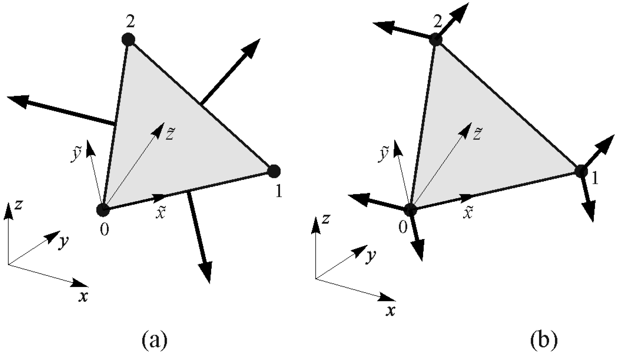
2.4. Stress Presentation over Nodal Forces

When the stresses at all Gaussian integration points of the corresponding triangular FE are determined, the internal forces laterally acting on the finite element may be calculated.

Components of the normal forces of the examined FE are given by:

$$\begin{array}{l}{n}_{\tilde{x}}={\displaystyle \underset{-t/2}{\overset{t/2}{\int }}{\sigma }_{\tilde{x}\tilde{x}} d\tilde{z}+{\mu }_a t {\dot{\epsilon }}_{\tilde{x}\tilde{x},c}\approx \frac{t}{2}{\displaystyle {\displaystyle \sum }_{i=1}^n{\sigma }_{\tilde{x}\tilde{x},i} w_i}}+{\mu }_a t {\dot{\epsilon }}_{\tilde{x}\tilde{x},c}\\ n_{\tilde{y}}={\displaystyle \underset{-t/2}{\overset{t/2}{\int }}{\sigma }_{\tilde{y}\tilde{y}} d\tilde{z}+{\mu }_a t {\dot{\epsilon }}_{\tilde{y}\tilde{y},c}\approx \frac{t}{2}{\displaystyle {\displaystyle \sum }_{i=1}^n{\sigma }_{\tilde{y}\tilde{y},i} w_i}}+{\mu }_a t {\dot{\epsilon }}_{\tilde{y}\tilde{y},c}\\ n_{\tilde{x}\tilde{y}}={\displaystyle \underset{-t/2}{\overset{t/2}{\int }}{\sigma }_{\tilde{x}\tilde{y}} d\tilde{z}+{\mu }_a t {\dot{\epsilon }}_{\tilde{x}\tilde{y},c}\approx \frac{t}{2}{\displaystyle {\displaystyle \sum }_{i=1}^n{\sigma }_{\tilde{x}\tilde{y},i} w_i}}+{\mu }_a t {\dot{\epsilon }}_{\tilde{x}\tilde{y},c}\end{array}$$

(36)

where w_i represents the weight coefficients, whereas n represents the number of Gaussian integration points. The last term in the Equation (36) represents the contribution of damping where μ_a is the normal damping coefficient, whereas $\stackrel{.}{\epsilon }$_ij (i,j = $\tilde{x}$,$\tilde{y}$) is the deformation rate. Critical normal damping μ_a,cr for the highest normal frequency in the system is presented by [25]:

$${\mu }_{a,cr}=\frac{2}{\sqrt{3}}h\sqrt{E\rho }$$

(37)

with h being the average height of the triangular finite element. The normal forces over the corresponding edge of the triangle in the direction of the local coordinate system, as displayed in Figure 4a, are presented as follows:

$$\begin{array}{l}{s}_{\tilde{x}}=n_{\tilde{x}\tilde{x}}{t}_{\tilde{x}}+n_{\tilde{x}\tilde{y}}{t}_{\tilde{y}}\\ s_{\tilde{y}}=n_{\tilde{y}\tilde{x}}{t}_{\tilde{x}}+n_{\tilde{y}\tilde{y}}{t}_{\tilde{y}}\end{array}$$

(38)

where t_$\tilde{x}$ and t_$\tilde{y}$ are the components of the normal on the edge of the deformed configuration of the triangle. Traction forces acting on the observed triangular edge are distributed in the corresponding nodes in the form of equivalent nodal forces, as displayed in Figure 4b.

Bending moments on the triangular element A are presented by:

$$\begin{array}{l}{m}_{\tilde{x}}={\displaystyle \underset{-t/2}{\overset{t/2}{\int }}{\sigma }_{\tilde{x}\tilde{x}} \tilde{z} d\tilde{z}+\left({\dot{\kappa }}_{\tilde{x}}+v{\dot{\kappa }}_{\tilde{y}}\right){\mu }_b\approx \frac{t}{2}{\displaystyle {\displaystyle \sum }_{i=1}^n{\sigma }_{\tilde{x}\tilde{x},i} {\tilde{z}}_i w_i}}+\left({\dot{\kappa }}_{\tilde{x}}+v{\dot{\kappa }}_{\tilde{y}}\right){\mu }_b\\ m_{\tilde{y}}={\displaystyle \underset{-t/2}{\overset{t/2}{\int }}{\sigma }_{\tilde{y}\tilde{y}} \tilde{z} d\tilde{z}+\left({\dot{\kappa }}_{\tilde{y}}+v{\dot{\kappa }}_{\tilde{x}}\right){\mu }_b\approx \frac{t}{2}{\displaystyle {\displaystyle \sum }_{i=1}^n{\sigma }_{\tilde{y}\tilde{y},i} {\tilde{z}}_i w_i}}+\left({\dot{\kappa }}_{\tilde{y}}+v{\dot{\kappa }}_{\tilde{x}}\right){\mu }_b\\ m_{\tilde{x}\tilde{y}}={\displaystyle \underset{-t/2}{\overset{t/2}{\int }}{\sigma }_{\tilde{x}\tilde{y}} \tilde{z} d\tilde{z}+\left(1-v\right) {\dot{\kappa }}_{\tilde{x}\tilde{y}}{\mu }_b\approx \frac{t}{2}{\displaystyle {\displaystyle \sum }_{i=1}^n{\sigma }_{\tilde{x}\tilde{y},i} {\tilde{z}}_i w_i}}+\left(1-v\right) {\dot{\kappa }}_{\tilde{x}\tilde{y}}{\mu }_b\end{array}$$

(39)

The last part of the Equation (39) represents the contribution of damping, whereas μ_b is the damping coefficient due to bending, while κ_ij (i,j = $\tilde{x}$,$\tilde{y}$) is the rate of change of curvature. The critical bending damping μ_b,cr for the highest normal frequency in the system is presented by [25]:

$${\mu }_{b,cr}=\frac{2}{\sqrt{18}}{t}^{2}h\sqrt{\frac{E\rho }{1-{\nu }^2}}$$

(40)

Ultimately, the moment m_n on the respective side of the examined triangular element, as displayed in Figure 5a, is presented by:

$$m_{nA}=m_x{\left(\frac{t_{\tilde{x}}}{\left|t_{\tilde{x}}\right|}\right)}^2+m_y{\left(\frac{t_{\tilde{y}}}{\left|t_{\tilde{y}}\right|}\right)}^2+2m_{\tilde{x}\tilde{y}}\frac{t_{\tilde{x}} t_{\tilde{y}}}{\left|t_{\tilde{x}}\right| \left|t_{\tilde{y}}\right|}$$

(41)

Moment m_n is then transformed into nodal forces presented by:

$$\begin{array}{l}{f}_2=\frac{m_{nA} l}{h_A} , f_{0A}=f_2\frac{l_{A2}}{l} , f_{1A}=f_2\frac{l_{A1}}{l}\\ f_3=\frac{m_{nA} l}{h_A} , f_{0B}=f_3\frac{l_{B2}}{l} , f_{1B}=f_3\frac{l_{B1}}{l}\end{array}$$

(42)

acting perpendicularly on the plane of the examined finite element A and the neighbouring finite element B, as displayed in Figure 5b. The procedure is reiterated for each side of the examined FE, and then for each FE. The forces derived from the moment are subsequently added to the global nodal force matrix.

2.5. Time Integration of Transient Dynamics

The time integration of transient dynamics is solved explicitly for each degree of freedom. The dynamic equation for each degree of freedom is, hence, presented by

$$m_i a_i=f_i$$

(43)

where m_i, a_i and f_i are the mass, acceleration, and total force which correspond to the i-th degree of freedom, respectively.

The time integration of the dynamic equation is solved by using the central difference time integration scheme, which is given by [25]:

$$\begin{array}{l}{v}_{i,t+\Delta t/2}=v_{i,t-\Delta t/2}+\Delta t f_{i,t}/m_i\\ x_{i,t+\Delta t}=x_{i,t}+\Delta t v_{i,t+\Delta t/2}\end{array}$$

(44)

where Δt is time step, while v_i and x_i are velocity and coordinates of i-th degree of freedom, respectively.

3. Numerical Verification

The previously described model has been applied to program Y based on the combined FDEM. The model was validated by using simple benchmark tests whereby the results were compared with the analytical and reference solutions available in the literature. Reference solutions were obtained by the programme package ABAQUS [34] using S3 and/or S4R finite elements. Both S3 and S4R are general-purpose shell elements with six DOFs per node. They use thick shell theory and are suitable for the large-strain geometrical nonlinear analysis. S3 are three-noded fully integrated triangular shell elements, while S4R are quadrilateral four-noded elements that use reduced integration with only one integration location. In the nonlinear solution procedure, the full Newton–Raphson method is used. The default convergence criteria are adopted with 0.5% force tolerance and 1.0% displacement tolerance. The default automatic load incrementation scheme is also adopted.

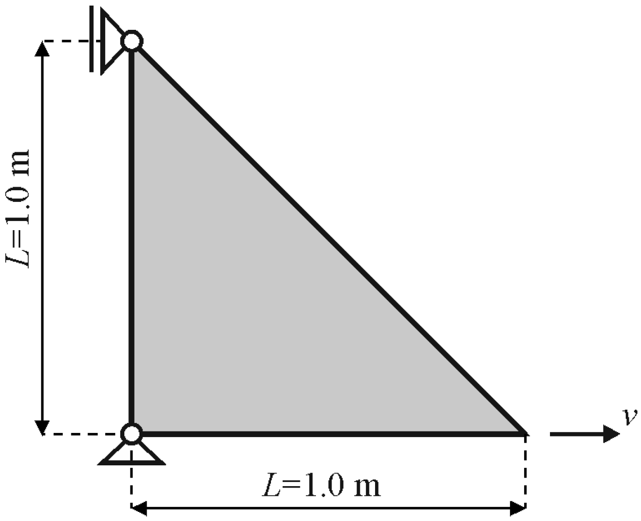
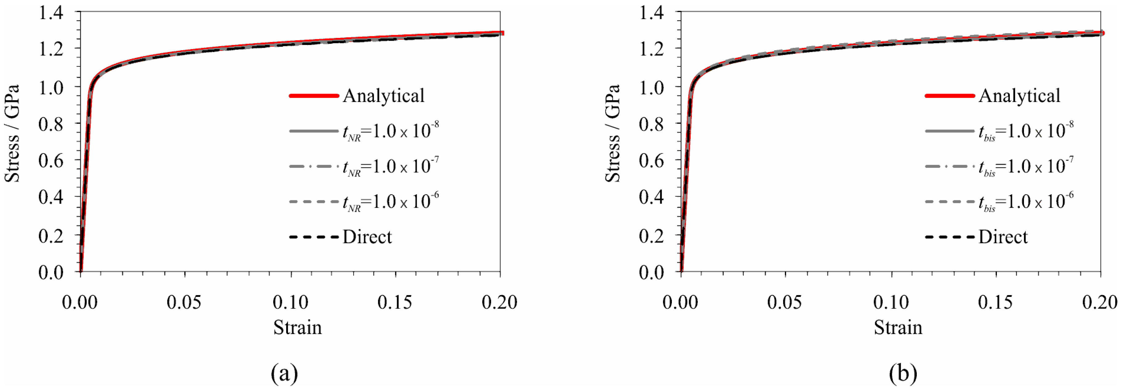
3.1. Uniaxial Tensile Test

This example was selected to verify the influence of the computational approach and the value of the tolerance error ε for the evaluation of the plastic correction parameter Γ on the accuracy and computational efficiency of the numerical solution. To this intent, the triangular element, as displayed in Figure 6, is subjected to the uniaxial loading accomplished by velocity v = 0.2 m/s at the right free end.

The analyses were performed by directly evaluating Γ via Equation (32), and by using the Newton–Raphson and the bisection iterative procedure with the tolerance error ε varied in the amount of 1 × 10⁻⁸, 1 × 10⁻⁷, and 1 × 10⁻⁶. All numerical results were compared with the analytical solution. The material properties of the triangle are adopted from Ming and Pantalé [32] and are summarised in

Table 1. Steel material properties.

E, GPa	ν	A, MPa	B, MPa	n
206.9	0.29	806	614	0.168

.

Figure 7a,b show the stress–strain relations in the triangle obtained by the Newton–Raphson and the bisection iterative procedures, respectively, varying the tolerance error t, in comparison with the direct approach for the evaluation of Γ and the analytical solution. It derives from above that all numerical results are very close to the analytical solution.

Table 2. Comparison of results for single element under tensile loading.

	Rel. Error (%)	Iterations
tbis = 1 × 10−8	0.24	19.982
tbis = 1 × 10−7	0.42	16.000
tbis = 1 × 10−6	1.23	13.000
tNR = 1 × 10−8	0.24	2.993
tNR = 1 × 10−7	0.28	1.996
tNR = 1 × 10−6	0.74	1.000
Direct	0.78	1.000

shows the absolute values of the relative error of stresses varying the computational approach and the tolerance error t for the evaluation of the plastic correction parameter Γ. Index bis in the table refers to the bisection method, while index NR refers to the Newton–Raphson method. All values in the table correspond to the strain equal to 0.2. Table 2 also presents the average number of iterations within the time step for the evaluation of Γ during the entire calculation process.

It derives from the presented results that by decreasing the tolerance error t, the accuracy of the numerical solution and the average number of iterations increases regardless of the selected iteration method. In addition, it derives that for the same value of the tolerance error t, more accurate solutions are procured from the Newton–Raphson method as compared to the bisection method. With a tolerance error t = 1 × 10⁻⁷, the Newton–Raphson method provides the solution with an accuracy of 0.28% and an average of 1.996 iterations per time step, while the bisection method provides the solution with an accuracy of 0.42% and an average of 16.00 iterations per time step. The direct solution method provides the solution with an accuracy of 0.78%. Adopting a 0.5% error as acceptable, it can be concluded that, in terms of computational efficiency, it is recommended the Newton–Raphson iterative procedure be used for the evaluation of the plastic correction parameter Γ with a tolerance error t_NR = 1 × 10⁻⁷.

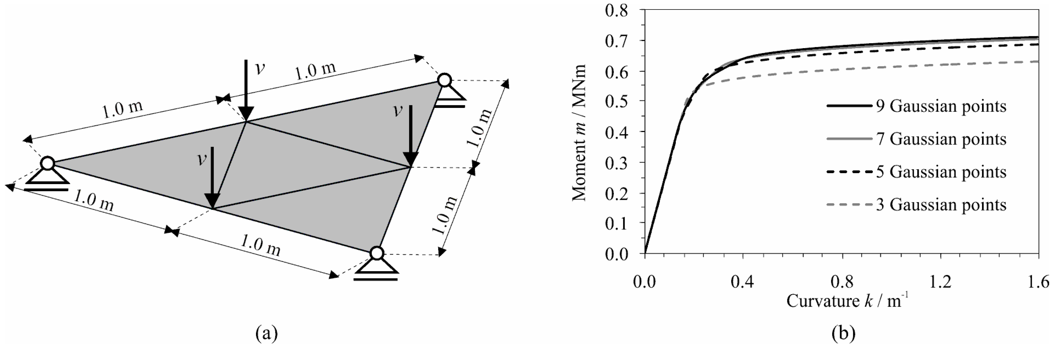
3.2. Four-Element Bending Test

This example analyses the impact of an error in the calculation of moments in the cross-section, depending on the number of Gaussian points. To this intent, a triangle plate discretised with four triangular finite elements simply supported at three corners, as presented in Figure 8a, was exposed to the bending loading condition, which was achieved by imposing velocity v = 0.01 m/s at the nodes of the central triangular element. The analyses were conducted for 3, 5, 7, and 9 Gaussian points. The thickness of the plate was equal to 5.0 cm, and the material properties of the elements are presented in Table 1.

Figure 8b plots the bending moment at the edge of the centre FE against the corresponding curvature varying the number of Gaussian points. It derives from the presented results that a greater number of Gaussian points increases the value of the plasticity moment. This is due to the fact that the use of more Gaussian points enables a more accurate determination of the part of the cross-section in which the material flows.

Table 3. Comparison of results for four elements under bending.

	Moment, MNm	Rel. Error (%)
3 Gaussian points	6.2967	11.29
5 Gaussian points	6.8607	3.34
7 Gaussian points	7.0275	0.99
9 Gaussian points	7.0981	-

shows the edge moment and the relative error of the moment at the end of the calculation adopting the moment obtained with nine Gaussian points as a reference solution. With seven Gaussian points, the relative error is less than 1.0%. It is expected that using nine Gaussian points will give a solution with an accuracy greater than 0.5%. More Gaussian points will lead to a more accurate numerical solution; however, the calculation time will also linearly increase. Therefore, it is necessary to find a minimum number of Gaussian points that will produce an error with acceptable accuracy. Adopting a 0.5% error as acceptable, it can be concluded that, in terms of computational efficiency, using nine Gaussian points within the cross-section is recommended.

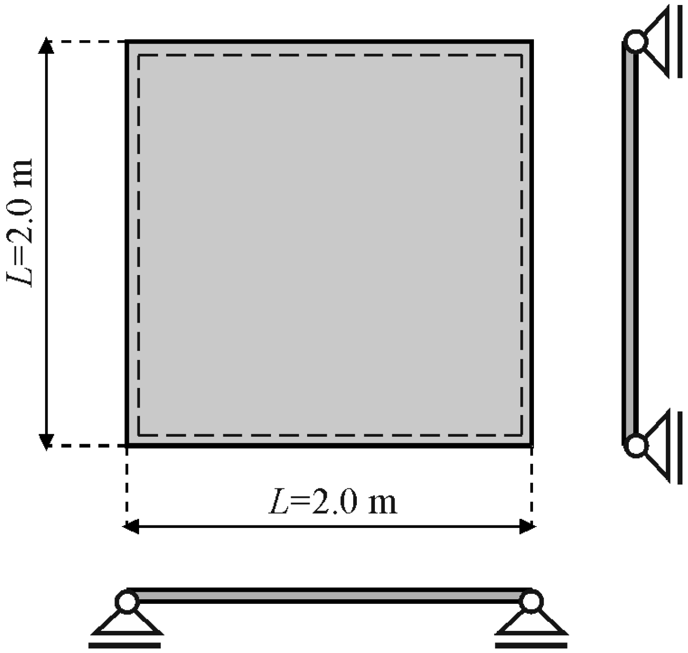
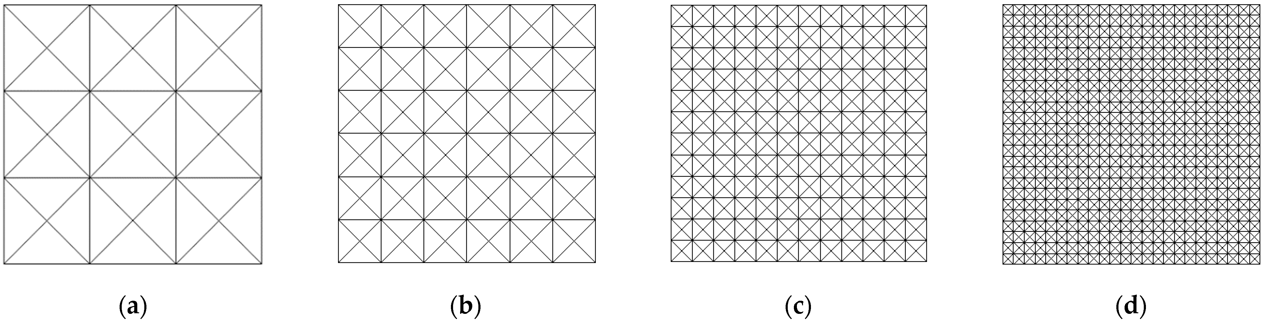
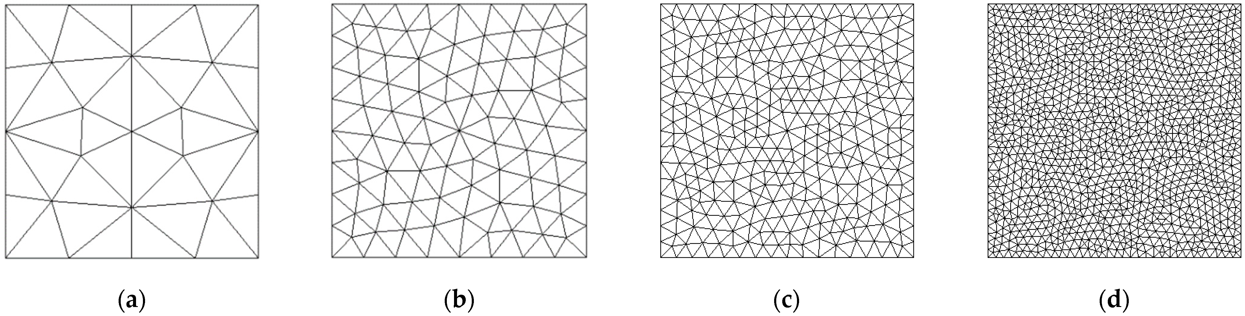
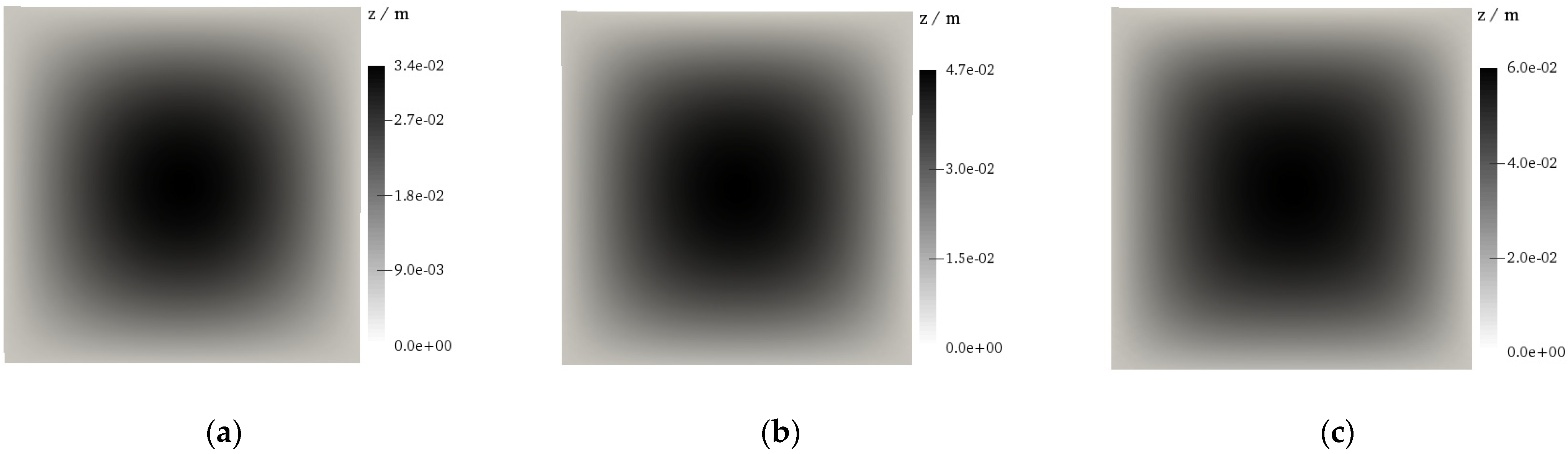
3.3. Square Plate Subjected to Gravity Load

In this example, the convergence of the numerical solution was analysed depending on the refinement and pattern of the FE mesh. For that purpose, the rectangular plate, with its geometry shown in Figure 9, was subjected to gravity load. The plate thickness amounted to 4 mm, while the material was linearly elastic, with the following properties: Poisson’s ratio ν = 0.3, Young’s modulus E = 210 GPa and density ρ = 7850 kg/m³. Gravity constant was g = 10.0 m/s².

The analyses were conducted by implementing the structured and unstructured finite element (FE) meshes with four refinements each, as displayed in Figure 10 and Figure 11, respectively.

Table 4. Central Deflection d (mm) of the plate and the relative error.

Average Length of the FE Sides	NDOF		Deflection d, mm		Relative Error, %
	FE Mesh Pattern		FE Mesh Pattern		FE Mesh Pattern
	Structured	Unstructured	Structured	Unstructured	Structured	Unstructured
h = L/4	75	81	8.87636	8.33342	2.19	8.85
h = L/8	255	294	9.06101	8.93905	0.10	1.47
h = L/16	969	1014	9.07437	9.03185	0.04	0.43
h = L/32	3603	3597	9.06939	9.06250	0.01	0.09

shows the numerically obtained mid-span deflection derived from the proposed numerical model and the relative error compared to the reference solution. The reference solution, equalling 9.070515 mm, was obtained from the programme package ABAQUS [34] by using 6400 S4R FEs. In addition, Table 4 displays the number of degrees of freedom (NDOF) of FE meshes. The numerical solutions in the performed analyses were obtained with two integration points per section height.

The displayed results indicate that by increasing the refinement of the FE mesh, the obtained numerical solution converges to the reference solution regardless of the FE mesh pattern. However, it is observed that the obtained solution converges faster with the structured mesh in relation to the unstructured FE mesh. Considering the presented convergence to the reference solution with increasing FE mesh refinement, in the examples presented below, only one FE mesh suitable for the comparison with the examples adopted from the literature was used.

Figure 12 shows the relative error obtained with the presented numerical model compared to quadrilateral four-noded S4R and triangular three-noded S3 Abaqus shell finite elements in relation to the NDOF. The relative error obtained by the presented numerical model relates to that obtained with the structured finite element meshes shown in Figure 10. The same meshes were used for the numerical analyses with the S3 Abaqus finite elements. It derives from the presented results that the convergence rate of the presented numerical model outperforms the S3 and S4R general-purpose shell elements from the well-known commercial software package ABAQUS [34] in terms of the NDOF. For instance, the FE mesh with 196 S4R FEs, which yields 1350 DOFs, provides a solution with an error of 0.26%, whereas the mesh with 576 S3 FEs (displayed in Figure 11c), which yields 1938 degrees of freedom, gives a solution with an error of 1.21%. For the presented model with a structured FE mesh and 969 DOFs, the relative error amounts to 0.04%.

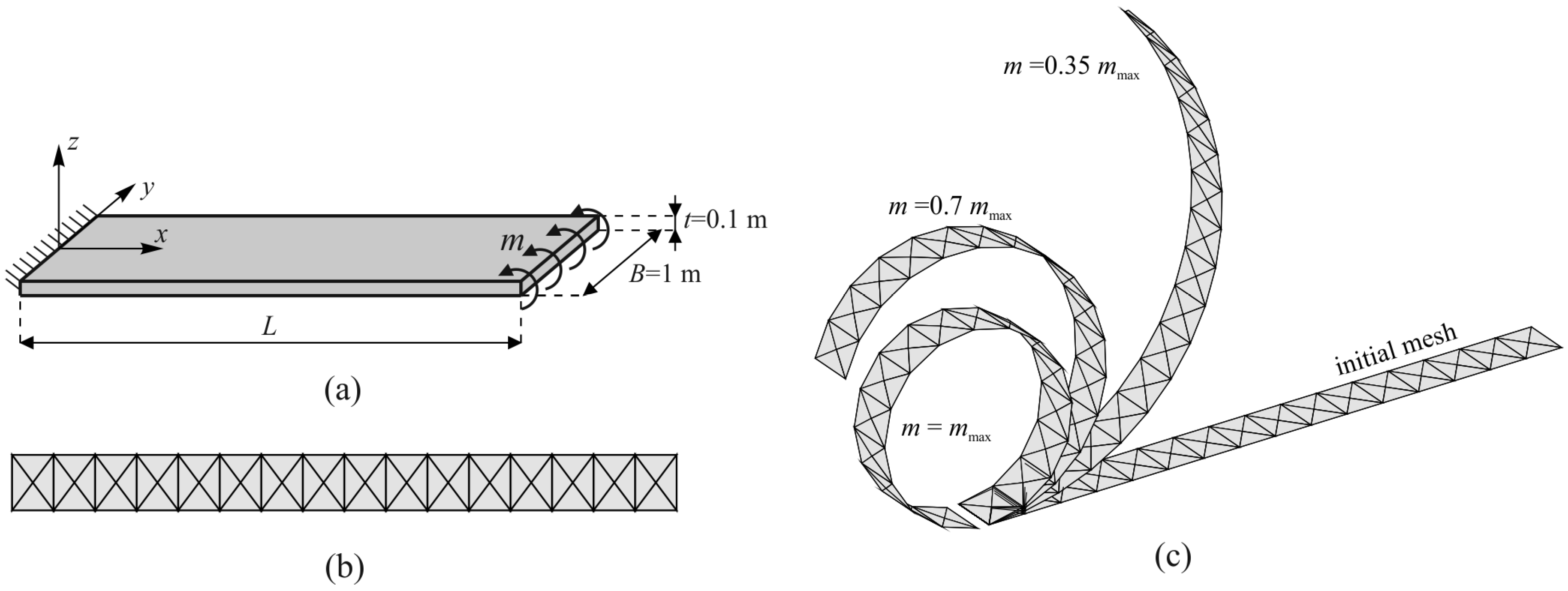
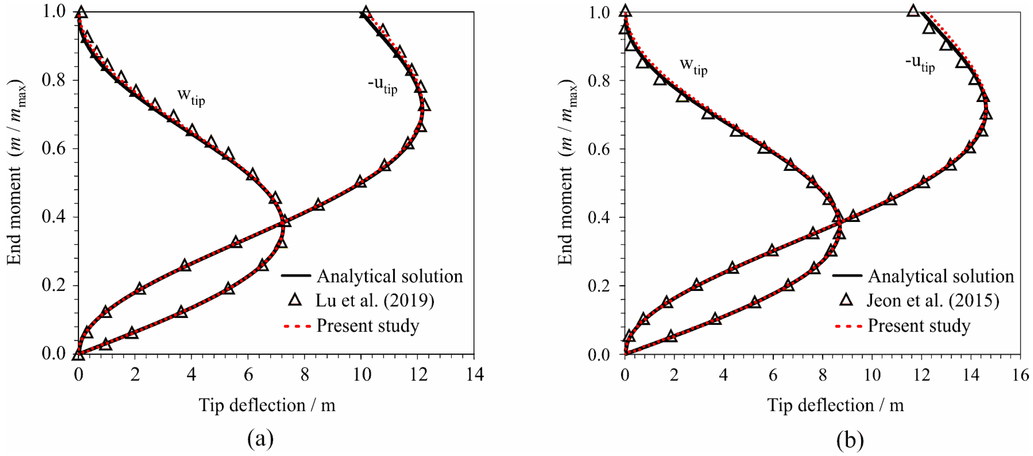
3.4. Cantilever Beam Exposed to End Moment

This example examines the suitability of the proposed numerical model for analysing problems with large rotations. For this purpose, a cantilever plate, whose geometry is displayed in Figure 13a, is exposed to end moment m. This issue is analysed in many references [35].

The material of the cantilever is linearly elastic with Young’s modulus and Poisson’s ratio, adopted in the amount of E = 1.2 MPa and v = 0, respectively. Under the moment at the free end m, the cantilever forms a circular arc with its radius R defined with the well-known flexural relation R = EI/m. Using this relation, the analytical tip deflections are obtained as:

$${\frac{u}{L}}_{}=\frac{m_0}{m} \sin \frac{m}{m_0}-1, {\frac{w}{L}}_{}=\frac{m_0}{m}\left(1-\cos \frac{m}{m_0}\right)$$

(45)

where m₀ = EI/L. The maximum end moment m_max is 2πm₀ at which the cantilever will bend into a circle. The analyses are performed with the lengths L = 10 m and L = 12 m. Figure 13b presents the FE mesh used in the performed analyses, which consists of 16 × 4 FEs, while Figure 13c shows the deformed configurations of the cantilever with the length L = 10 m at different stages. The central node in the presented finite element mesh is added because the spatial second order polynomial defined by relations (4) and (5), which approximates the cantilever geometry near the observed triangle, cannot be performed with only two nodes in one direction.

Figure 14a,b show the load–displacement curves for the cantilever with the lengths of 10 m and 12 m, respectively. For comparison purposes, the results from Lu et al. [36] and Jeon et al. [37] are also depicted in said figures. The results obtained from the presented numerical model match those obtained by Lu et al. [36] and Jeon et al. [37] and are reasonably close to the reference solutions.

In their analyses, Lu et al. [36] used 10 × 2 NLDGT three-noded triangular finite elements with 6 DOFs per node, while Jeon et al. [37] used 16 × 2 MITC3+ three-noded triangular FEs with 5 DOFs per node and 2 additional rotational degrees of freedom in the central node of the FE.

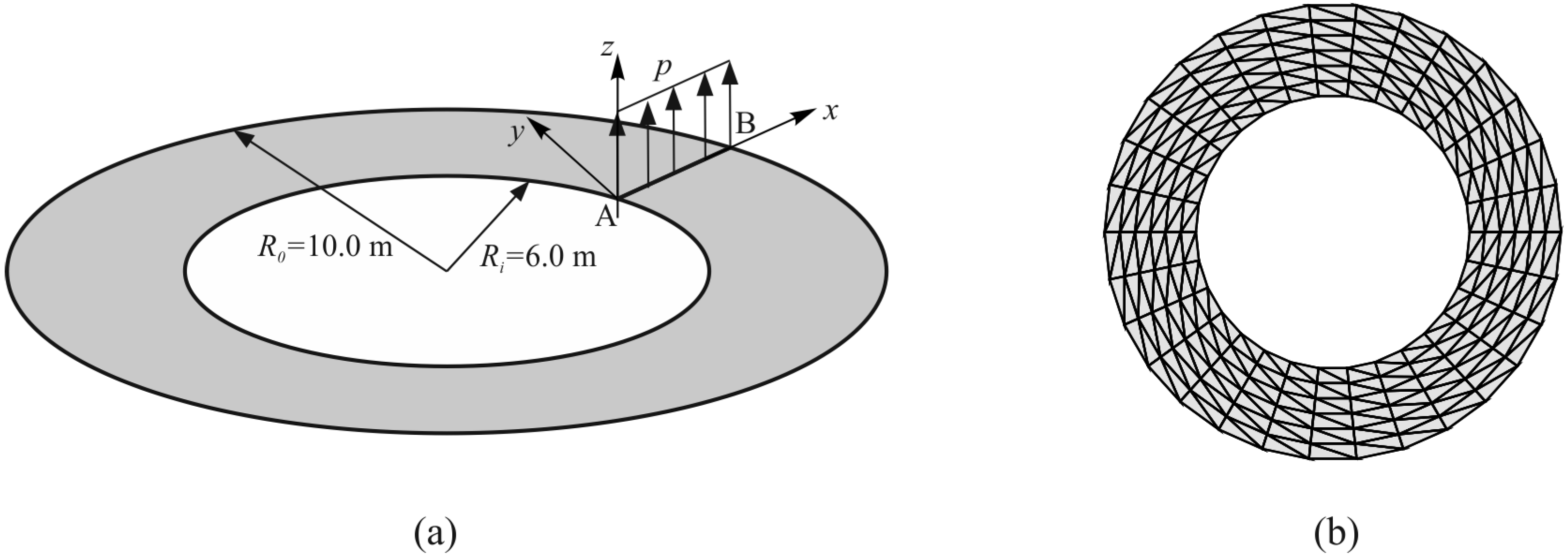
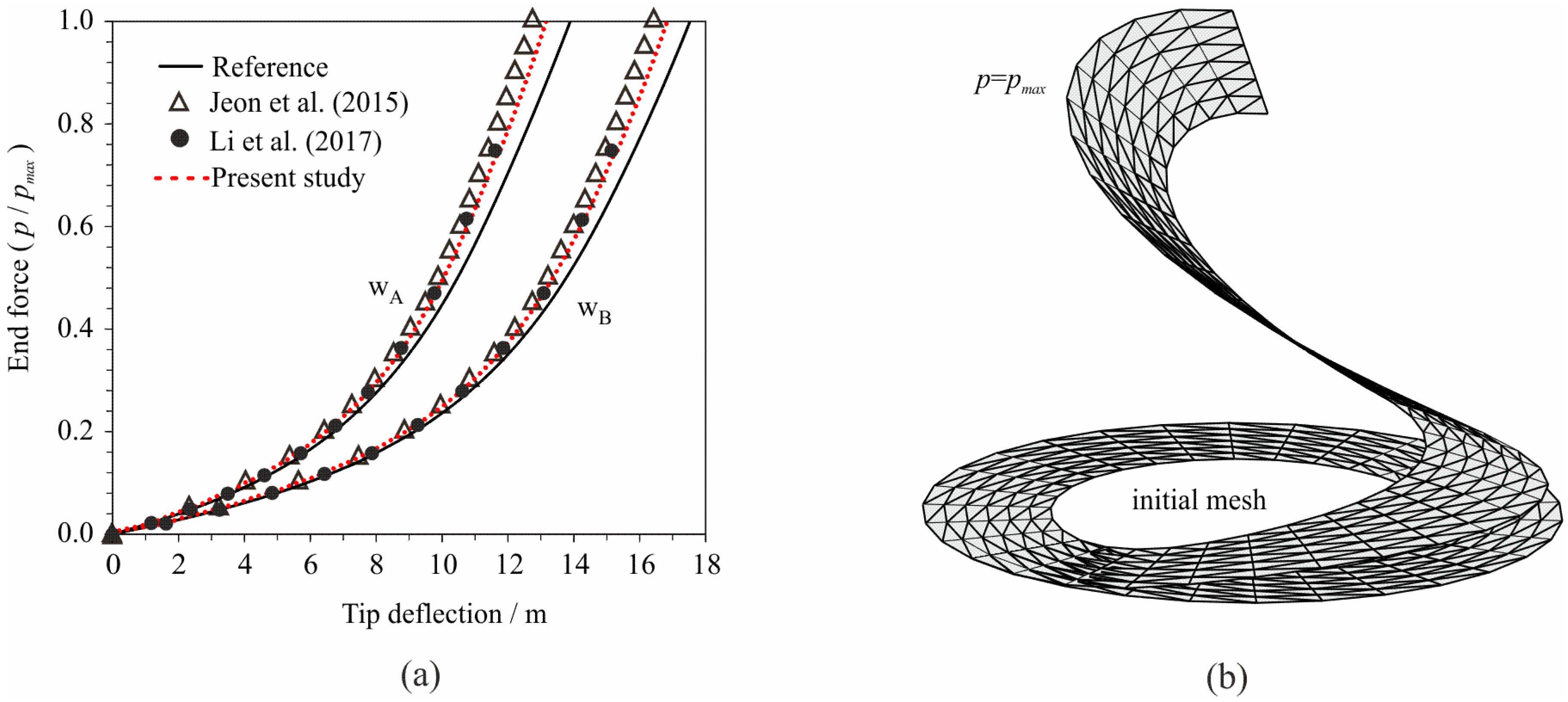
3.5. Slit Annular Plate Exposed to Lifting Force

The slit annular plate whose geometry is displayed in Figure 15a is exposed to the monotonic increasing line force p_max = 0.8 N/m at one end of the slit, while the other end of the slit is fully clamped. This issue has been considered in many references [35]. The thickness of the plate is 0.03 m, while the Poisson’s ratio and Young’s modulus equal v = 0.0 and E = 21.0 MPa, respectively.

Figure 15b displays the FE mesh used in the performed analyses, which consists of 6 × 32 × 2 finite elements.

The load–displacement curves at two different points, A and B, are shown in Figure 16a. For comparison purposes, the results from Jeon et al. [37] and Li et al. [10] are also depicted in this figure. It derives that the results obtained from the presented numerical model match those obtained by Jeon et al. [37] and Li et al. [10] and are reasonably close to the reference solutions. The reference solution [35] was obtained with the programme package ABAQUS by using 10 × 80 S4R shell FEs.

It should be noted that Jeon et al. [37] used 6 × 30 × 2 MITC3+ triangular finite elements with 5 DOFs per node and 2 additional rotational degrees of freedom in the central node, while Li et al. [10] used 4 × 32 × 2 TRIS3 three-noded triangular elements with 5 DOFs per node, which yielded 1255 DOFs and 825 DOFs, respectively. In this paper, we used 360 triangular three-noded FEs with 3 DOFs per node, which yielded 651 DOFs. Figure 16b shows the deformed mesh of the plate at p = p_max.

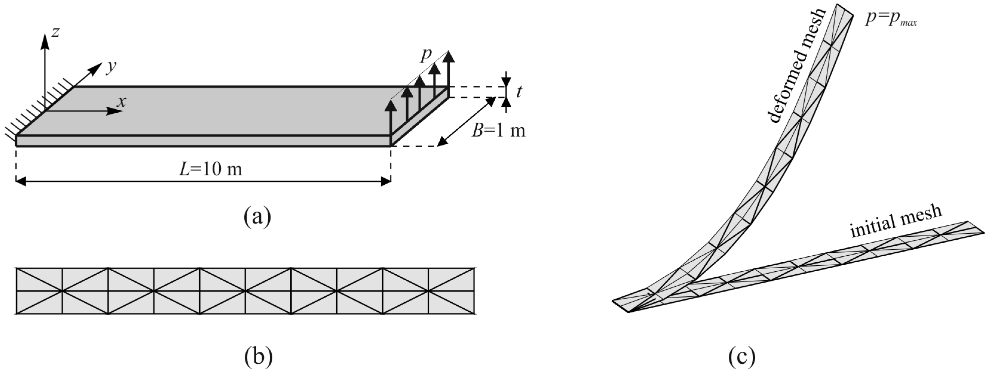
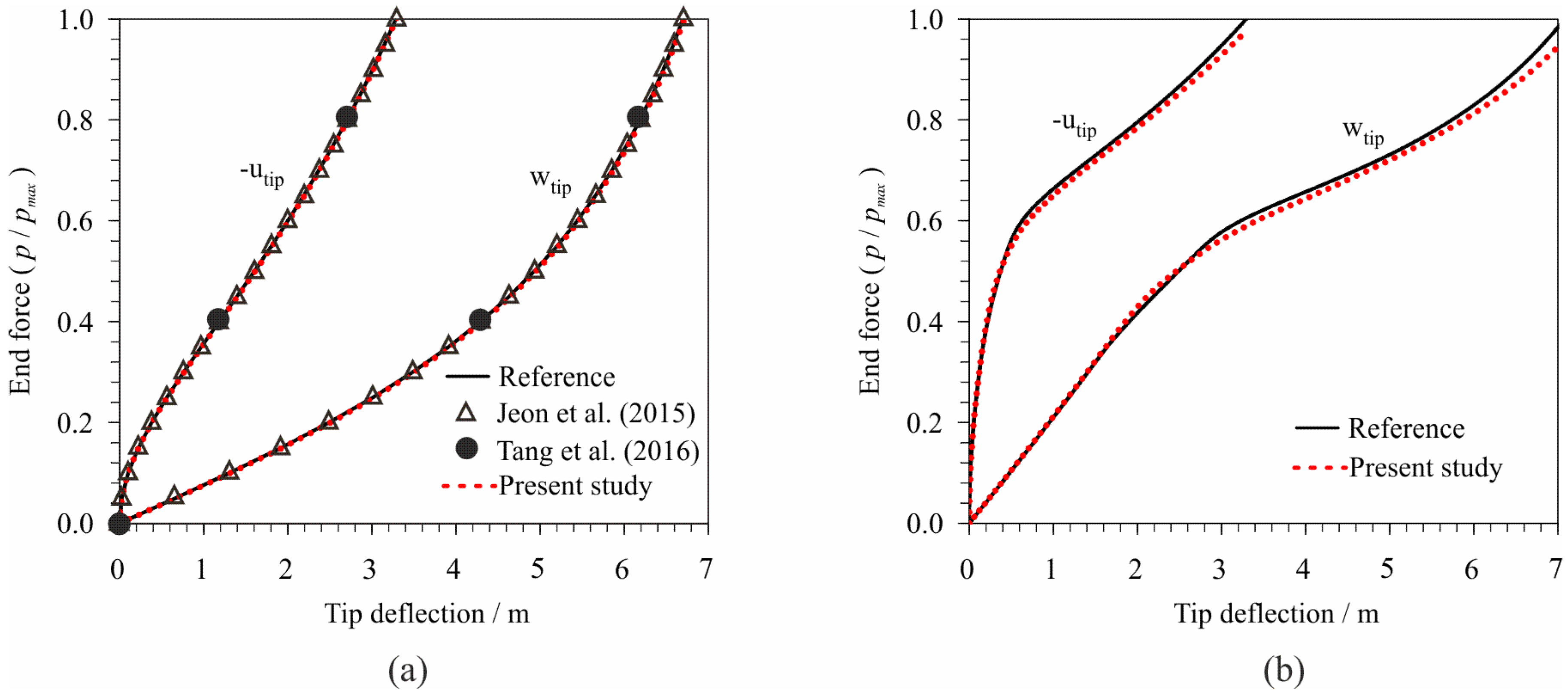
3.6. Cantilever Beam Exposed to End Shear Force

A cantilever plate with geometry displayed in Figure 17a is exposed to end shear force so as to additionally verify the large rotation and large displacement capacity of the presented numerical model. This issue has been analysed in many references [35].

In the present study, the analyses were performed with nonlinear and linear-elastic material behaviour. Material properties, geometry and applied force in the analysis with linear-elastic material behaviour are as follows: Young’s modulus of elasticity E = 1.2 MPa, and Poisson’s ratio v = 0, thickness t = 0.1 m, and maximal end shear force p_max = 4 N. In the analysis with nonlinear material, whose material properties are presented in Table 1, the adopted thickness t was 0.1 m, while the maximal end shear force was equal to p_max = 2.0 MN. The FE mesh used in the numerical analyses and displayed in Figure 17b consisted of 10 × 4 finite elements, while Figure 17c shows the deformed FE mesh for the linear material behaviour under the maximum force.

Figure 18a shows the horizontal (u_tip) and the vertical (w_tip) displacement of the cantilever tip relative to the vertical force for linear-elastic material behaviour in comparison with the reference solutions, i.e., three-noded triangular shell elements MITC3+ presented by Jeon et al. [37] and quadrilateral flat shell finite elements presented by Tang et al. [38]. Reference solution [35] was obtained with the programme package ABAQUS by using 16 × 1 S4R shell FEs with 6 DOFs per node, which yields 192 DOFs. It can be observed that the results of the presented shell element are in excellent agreement with the other elements. It should be noted that, in the same example, Jeon et al. [37] used 16 × 2 MITC3+ finite elements with 5 DOFs per node and 2 additional rotational degrees of freedom in the centre of the finite element, which yields 224 DOFs, while Tang et al. [38] used 10 × 1 quadrilateral four-noded FEs with 6 DOFs per node, which yields 120 DOFs. In this paper, we used 40 triangular three-noded FEs with 3 DOFs per node, which yields only 90 DOFs.

Figure 18b shows the horizontal (u_tip) and the vertical (w_tip) displacement of the cantilever tip relative to the vertical force for nonlinear material compared to reference solutions. The reference solution [35] in this case was obtained from the programme package ABAQUS by using 20 × 1 S4R FEs. It shows a very good agreement of the results with the reference solution.

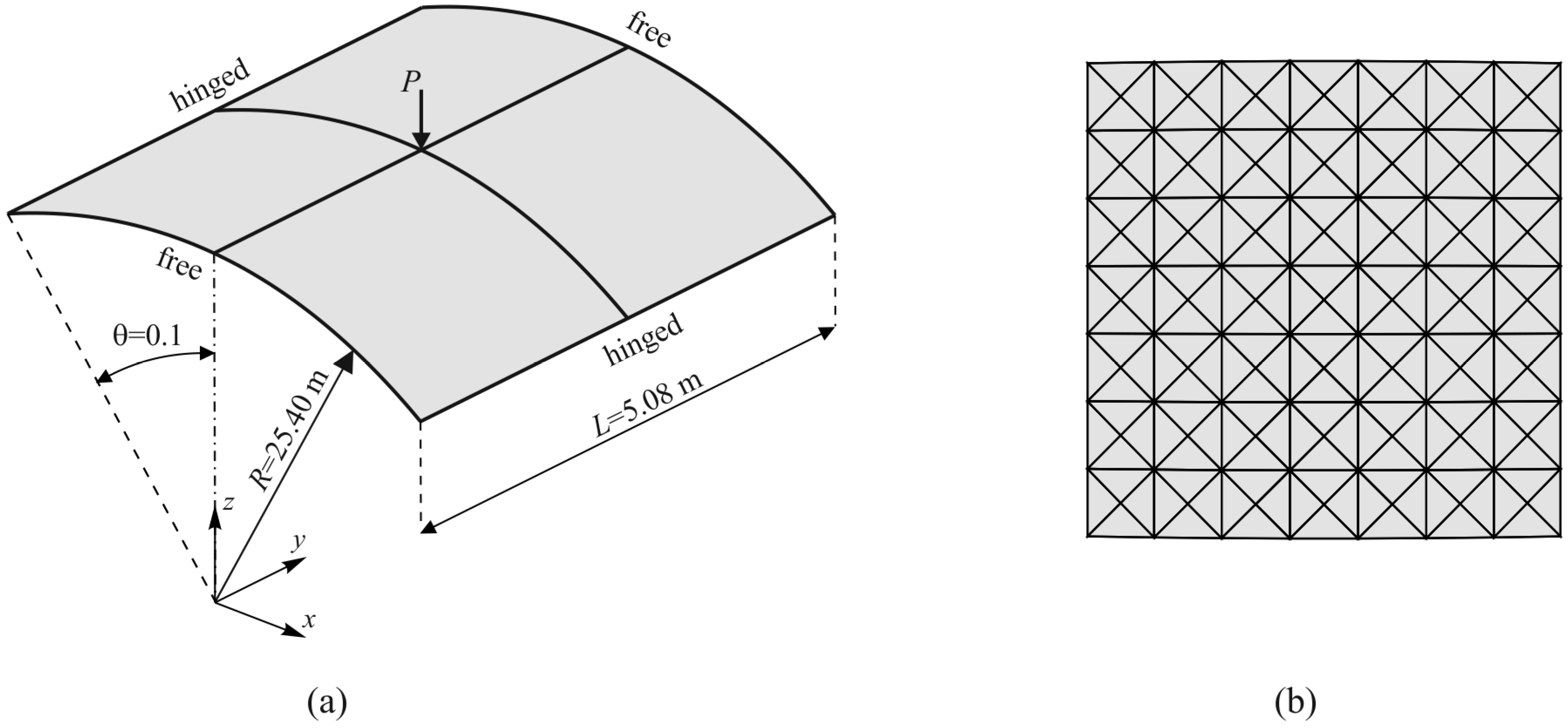
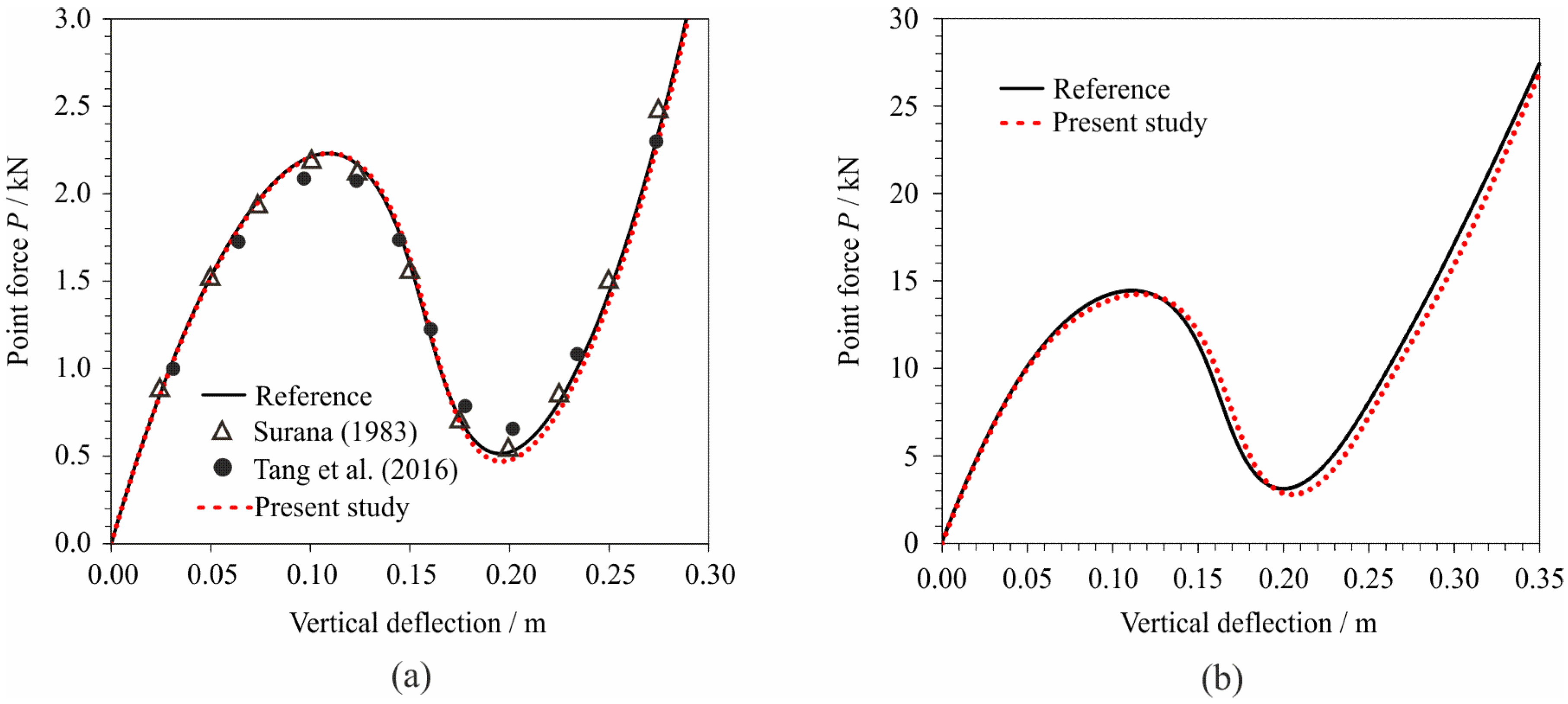
3.7. Hinged Cylindrical Roof under Monotonic Increasing Central Force

A hinged semi-cylindrical roof exposed to the central pinching force, which is popular due to the snapping behaviour, has been analysed in many references [35] considering linear-elastic material behaviour. The geometry and the loading condition of the roof are displayed in Figure 19a. The roof thickness is 12.7 cm. Along the hinged edges, all nodal translations are restrained. Within the present study, the analyses are performed with nonlinear material behaviour and linear-elastic material behaviour with the following properties: Poisson’s ratio v = 0.3 and Young’s modulus E = 31.0275 MPa. The nonlinear material characteristics are presented in Table 1. The FE mesh used in both analyses and presented in Figure 19b consists of 196 finite elements.

Figure 20a plots the comparison of the central pinching force against the central deflection for the linear-elastic material behaviour obtained from the presented numerical model compared to the reference solutions, i.e., quadrilateral flat shell finite elements presented by Tang et al. [38] and parabolic curved shell elements proposed by Surana [39]. The reference solution [35] is obtained from the programme ABAQUS by using 16 × 16 S4R shell FEs (for one-quarter of the shell) with 6 DOFs per node, which yields 1743 DOFs for the whole structure. It can be observed that the results of the presented shell element are in good agreement with other elements and the reference solutions. It should be noted that Tang et al. [38] used 4 × 4 quadrilateral four-noded FEs with 6 DOFs per node, while Surana [39] used 2 × 2 parabolic curved shell finite elements with 8 nodes and 5 DOFs per node for one-quarter of the shell, which yields 1730 DOFs and 405 DOFs, respectively, for the whole structure. In this paper, we used 40 triangular three-noded FEs with 3 DOFs per node, which yields 339 DOFs.

Figure 20b plots the comparison of the central pinching force against the central deflection for nonlinear material behaviour in comparison with the reference solution. In this case, the reference solution is obtained from the programme package ABAQUS [34] by using 25 × 25 S4R shell FEs for one-quarter of the shell. A relatively good agreement is observed between the obtained results and the reference solution. This indicates the suitability of the presented formulation in the analysis of the problems with snapping behaviour for both linear and nonlinear material behaviour.

3.8. Free Vibration of Hinged Cylindrical Roof under Constant Central Force

A hinged cylindrical roof with the same geometrical and material characteristic as in the previous example was exposed to free vibrations under the constant central force f = 12.0 MN to demonstrate the suitability of the proposed numerical formulation in the dynamic analysis of the structure. The analyses were performed with nonlinear and linear-elastic material behaviour, with the material properties displayed in Table 1. Two FE meshes were used in the performed analyses: the finite element mesh shown in Figure 19b, which consisted of 196 finite elements, and a finite element mesh with the same mesh pattern as the mesh in Figure 19b, but with 900 finite elements.

Figure 21 shows the comparison of central deflection in time for the linear-elastic and the nonlinear material behaviour obtained from the presented numerical model compared with the reference solution. As in the previous example, the reference solution was obtained from the programme package ABAQUS [34] by using 625 S4R FEs for one-quarter of the shell and explicit time integration of the motion equation.

In this example, it is evident that a FE mesh with 196 finite elements, which provided a rather good solution in the quasi-static analysis, is unable to provide such a good solution in the dynamic analysis. This is because, in the dynamic analysis, the higher forms of vibration produce the effects that can only be captured with a finer finite element mesh, such as the one with 900 finite elements. This influence of higher forms of vibration proved to be more pronounced in linear-elastic material than in nonlinear.

However, FE mesh with 900 finite elements provided a very good agreement of the results in comparison with the reference solution for both nonlinear and linear material behaviour, which indicates the suitability of the proposed numerical model for the dynamic analysis of shells with nonlinear and linear material behaviour.

Also, from the presented results, a significant difference in free vibrations can be observed between the nonlinear and linearly elastic material behaviour. In fact, although the maximum central shifts during the vibration of both materials are approximately the same, the nonlinear material oscillates with approximately three-and-a-half times smaller amplitudes and three times higher frequencies with respect to the linear material.

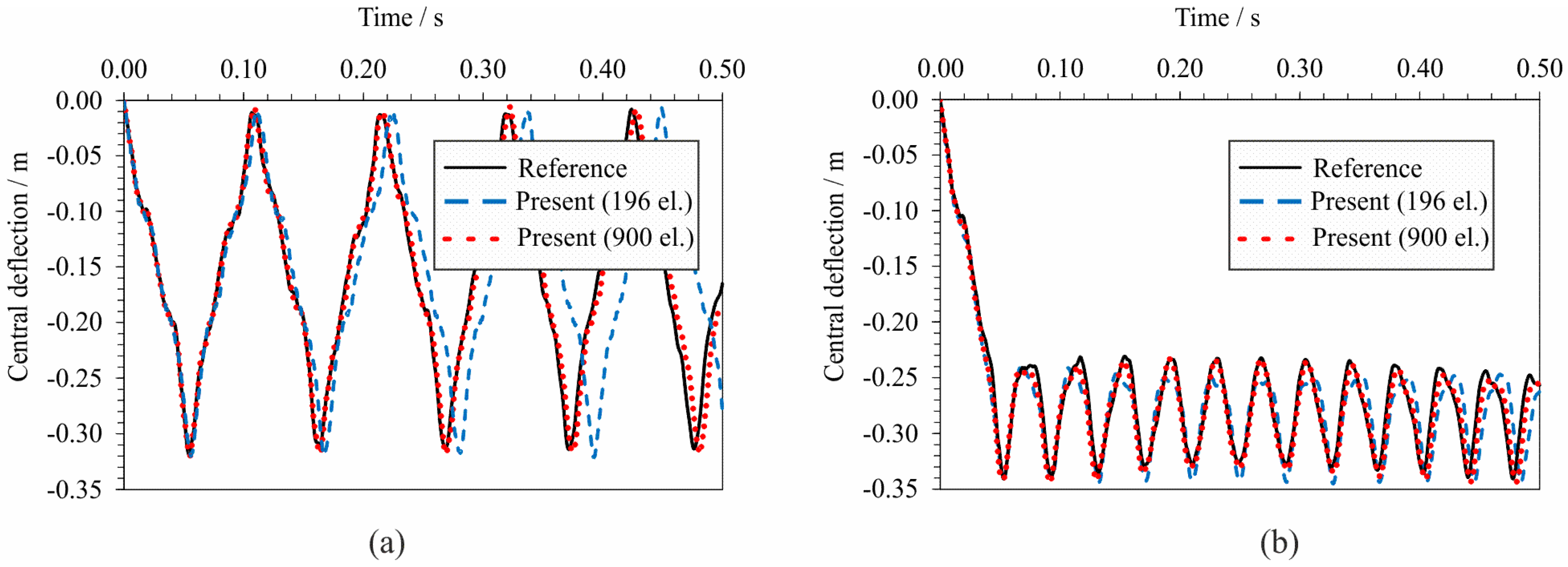
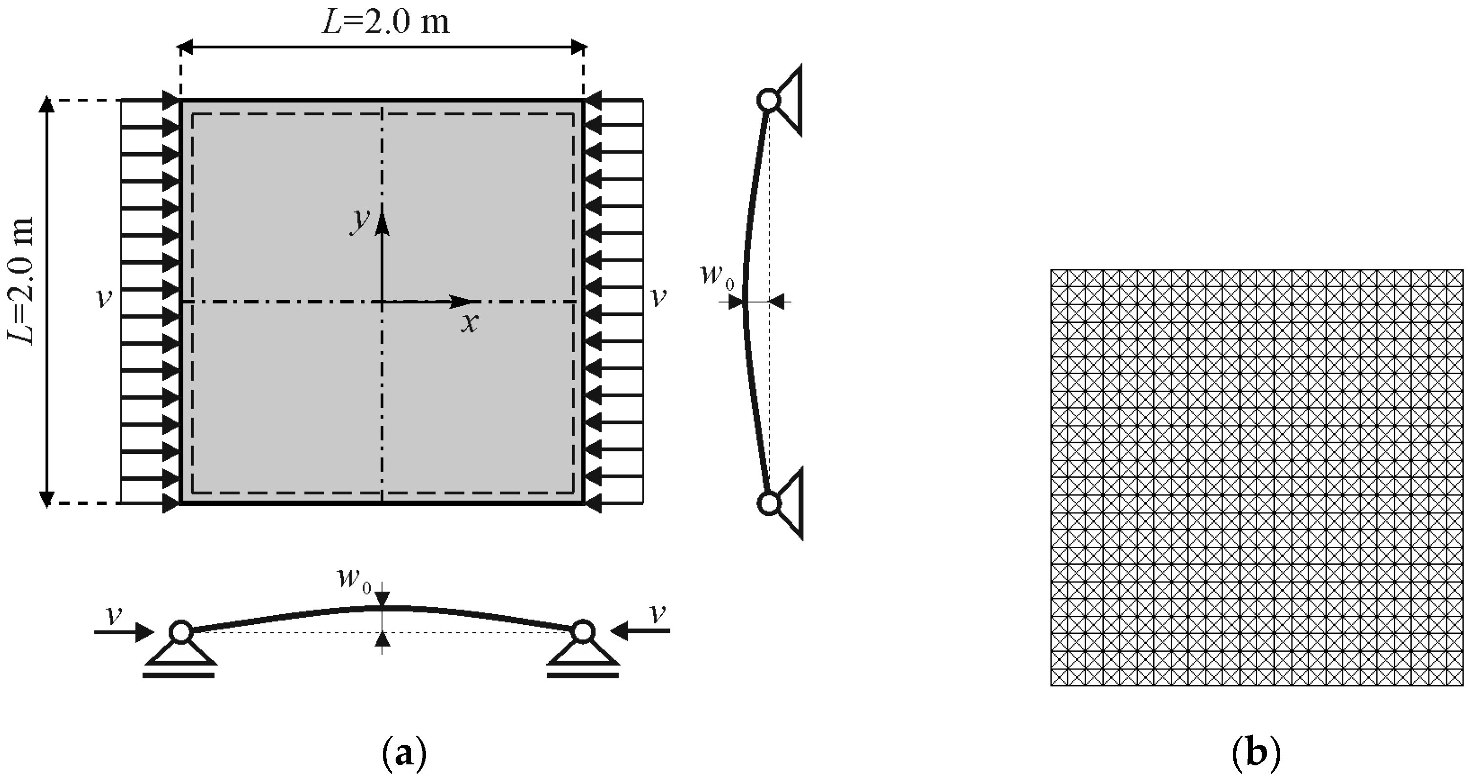
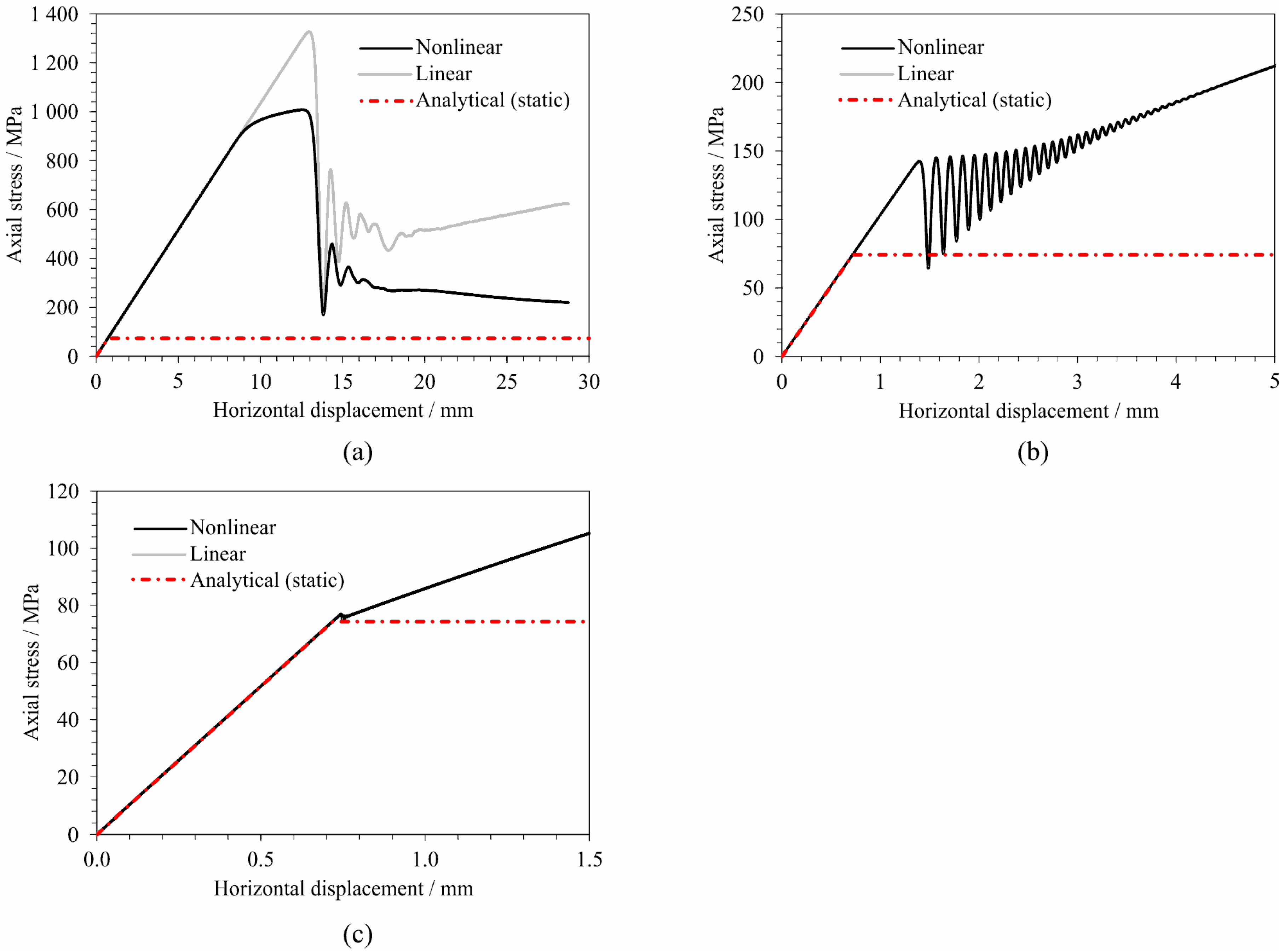
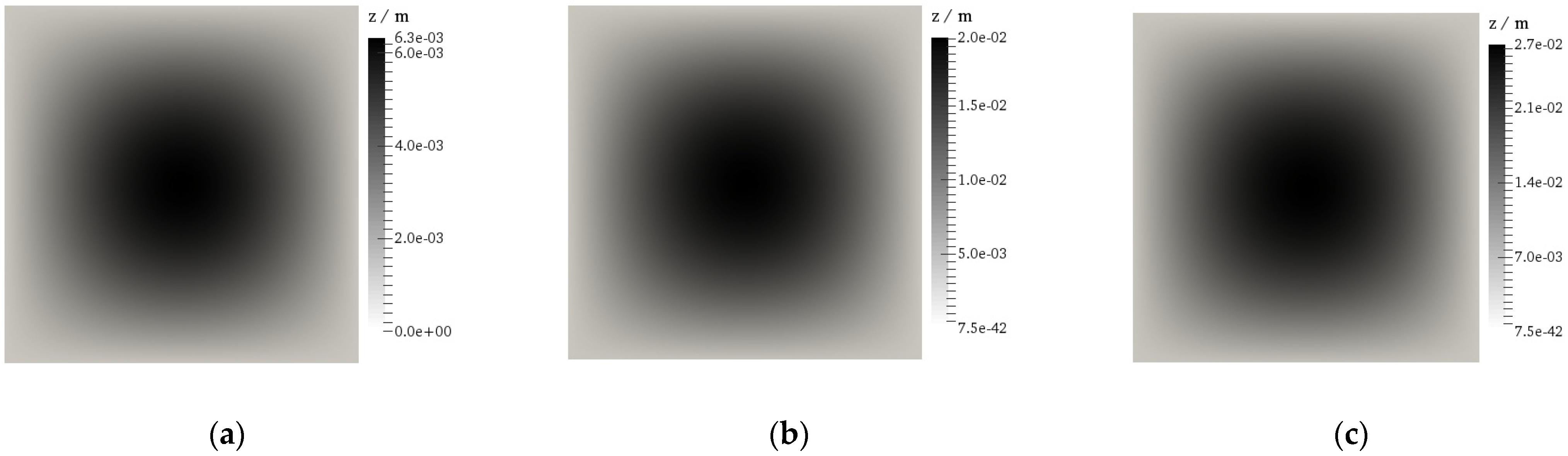
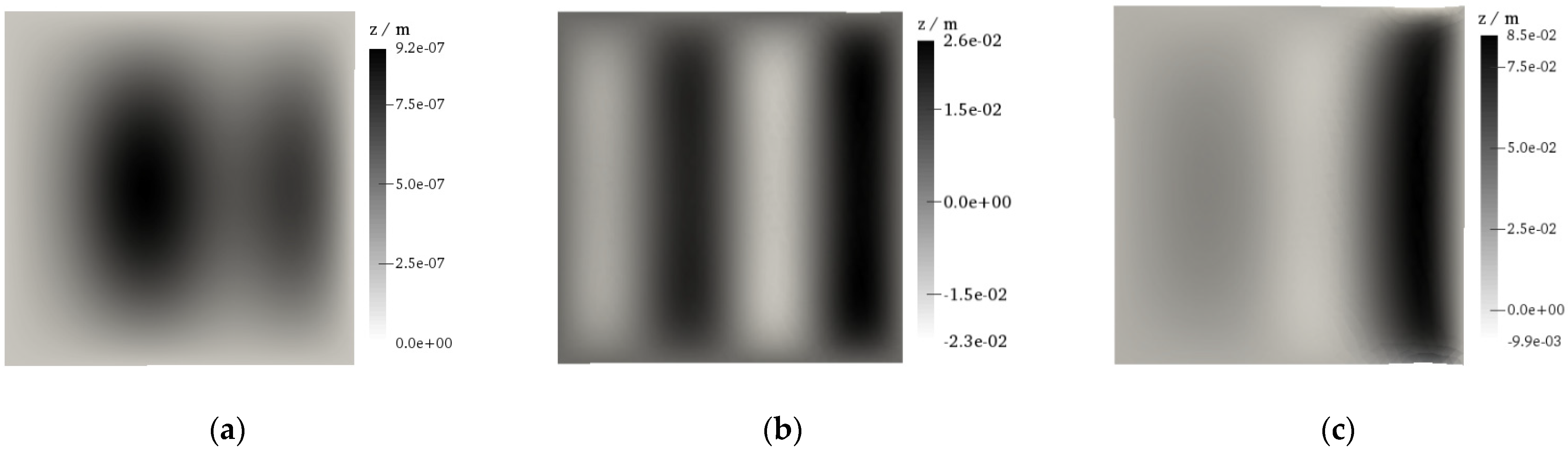
3.9. Buckling of Axially Loaded Rectangular Plate

A simply supported rectangular plate loaded with uniaxial compressive loading achieved by applying a constant velocity v at two opposite sides of the plate, as shown in Figure 22a, was selected for the application of the proposed numerical model in the stability analysis of the plates. In order to obtain the dynamic buckling effect, the velocity at the sides of the plate was varied and corresponded to the deformation rates of 2.5 × 10⁻¹ s⁻¹, 2.5 × 10⁻³ s⁻¹, and 2.5 × 10⁻⁵ s⁻¹. All analyses were performed with the nonlinear and linear-elastic material behaviour, with the material characteristic presented in Table 1.

The discretisation of the plate with the FE mesh is presented in Figure 22b. The thickness of the plate was 20 mm. In order to account for some extent of imperfection, the initial deflection of the plate was adopted as the cosine function:

$$w_i\left(x,y\right)=w_0 \cos \left(\frac{\pi x}{L}\right) \cos \left(\frac{\pi y}{L}\right)$$

(46)

with w₀ equal to w₀/L = 1.0 × 10⁻⁹. Equation (46) ensures that the initial imperfection at the edges of the plate is zero while at the rest of the plate it equals the cosine function with the highest value of w₀ at the centre of the plate.

The analytical solution of the presented problem [31] with the static loading conditions and the linear-elastic material behaviour provides the following equation for critical axial stress, due to which the plate loses its stability:

$${\sigma }_{x,cr}=\frac{{\pi }^{2}E}{3\left(1-{\upsilon }^2\right)}{\left(\frac{t}{L}\right)}^2$$

(47)

which, taking into account the concrete values related to geometrical and material characteristics, yields σ_x,cr = 74.31 MPa.

Figure 23 shows the relation between the average axial stress and the shortening of the plate for three values of strain rates. All solutions are compared with the critical stress obtained from the analytical solution.

It derives from the presented results that the increase in the strain rate also increases the dynamic buckling axial stress. In this specific case, for the strain rate of 2.5 × 10⁻¹ s⁻¹ and the linear-elastic material behaviour, the buckling axial stress is approximately 18 times higher as compared to the buckling axial stress at the strain rate of 2.5 × 10⁻⁵ s⁻¹. It can also be observed that for higher strain rates, in the specific case of 2.5 × 10⁻¹ s⁻¹, the buckling can appear after reaching the yielding stress, resulting in significantly lower buckling stress, considering the nonlinear material behaviour as compared to the buckling stress in materials with linear-elastic behaviour. This example further emphasises the need to consider material nonlinearities in the stability analysis of plate or shell structures due to the dynamic loading condition. It derives from the presented results that by decreasing the strain rate, the numerically obtained stress at which the plate loses stability converges according to the analytical solution obtained for the static activity. In this particular case, for the strain rate of 2.5 × 10⁻⁵ s⁻¹, the numerically obtained buckling axial stress is 2.5% higher as compared to the analytical solution; however, more accurate results could be obtained with smaller strain rates when the dynamic effects would be even less pronounced. Figure 24, Figure 25 and Figure 26 show the shape of the plate in different time steps after the buckling for strain rates 2.5 × 10⁻¹ s⁻¹, 2.5 × 10⁻³ s⁻¹, and 2.5 × 10⁻⁵ s⁻¹, respectively. It derives from the presented results that, at lower strain rates, the buckling occurs in the first eigenmode, while at higher strain rates, the buckling occurs at higher eigenmodes.

4. Conclusions

A new 4-TRINONL numerical model for the analyses of thin shells was presented. The model deals with nonlinear and linear material behaviour, taking into account large displacements, large rotations, and small strains. The discretisation of the structure within the proposed model is based on rotation-free three-noded finite elements. Material nonlinearity with hypo-elastic-based constitutive law is implemented by considering the von Mises yield criterion and the Levi–Mises flow rule. The presented numerical model uses an explicit time integration scheme for the integration of motion equation, but an implicit radial returning algorithm to compute the plastic strain at the end of each time step. The model has been embedded in Program Y based on the finite–discrete element method and tested on simple examples.

Pursuant to the conducted numerical examples and presented numerical formulations, the following conclusions have been drawn:

• The presented numerical model is appropriate for the dynamic, quasi-static, and stability analysis of thin shell structures.
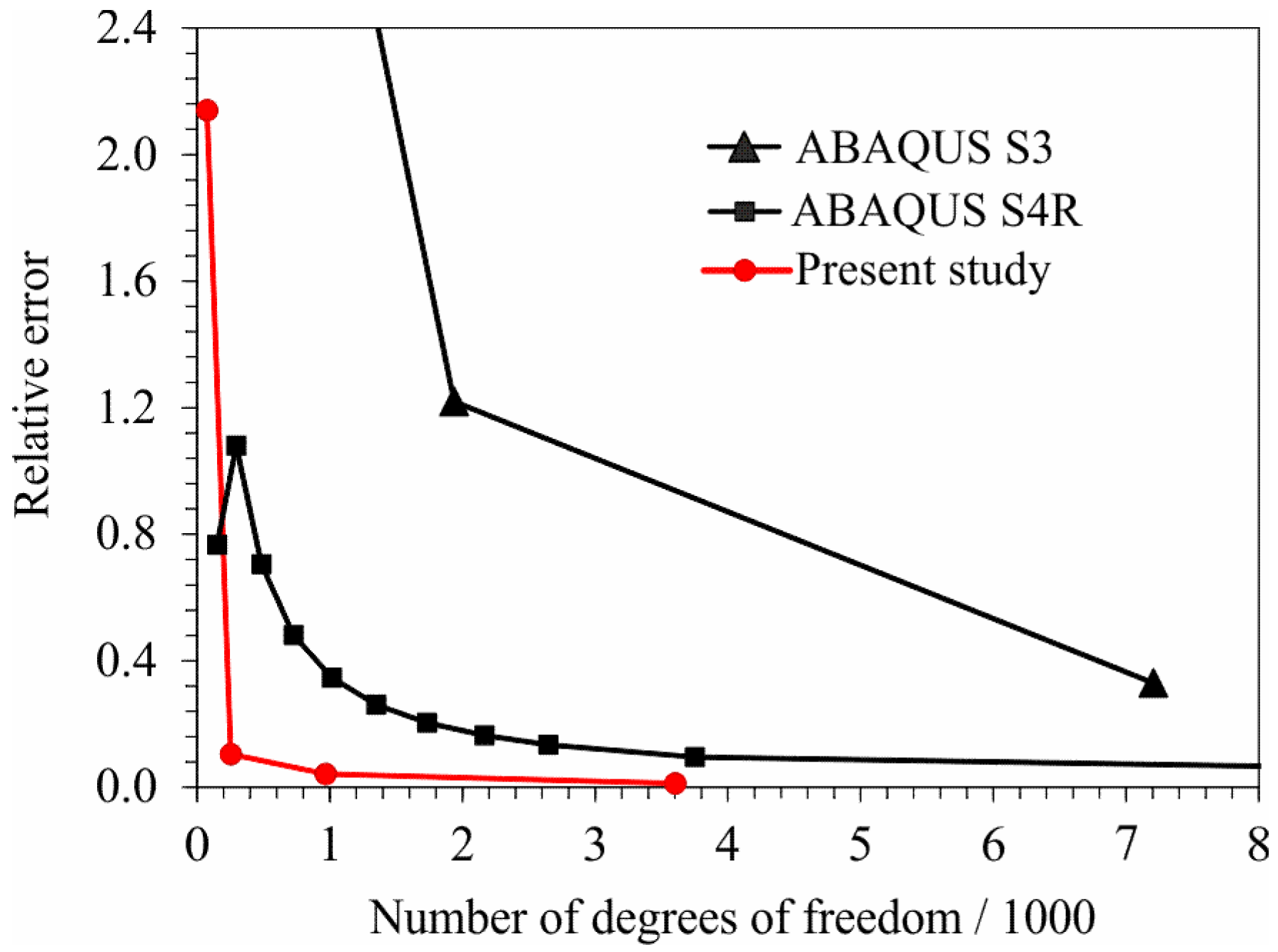
• In the tested examples, the performance of the proposed formulations is similar to or better than the one with standard triangular or quadrilateral shell elements measured in terms of the number of DOFs.
• Finally, it cannot be concluded that the presented numerical model is better or worse than other numerical models of a similar type or that it can do something that could not be done with other numerical models. However, one of the main advantages of the presented numerical model may be sought in the robustness of its formulation. Considering that the time integration transient dynamics is solved explicitly for each degree of freedom, there is no need for introducing stiffness and mass matrix at the system level or to solve the large-scale system of equations. The determination of stress and strain at the Gaussian integration points is based on the geometry of the control domain determined by the observed triangle and three neighbouring triangles, which implies that no information related to other triangular FEs in the system is required. In view of the above, the presented formulation seems appropriate for the parallel programming to be executed at the level of the control domain.

Moreover, the model can be easily upgraded for the purpose of interacting with the fracture or for the analysis of laminated shells with some other material constitutive law and finite strains, which is yet another advantage of using the FDEM model.

It should be noted that the procedures described in this paper are not intended for finite strains but are limited instead to thin shell structures subjected to small strains.

References

1. Bucalem, M.L.; Bathe, K.J. Finite element analysis of shell structures. Arch. Comput. Methods Eng. 1997, 4, 3–61. [Google Scholar] [CrossRef]
2. Stolarski, H.; Belytschko, T.; Lee, S.H. A review of shell finite elements and corotational theories. Comput. Mech. Adv. 1995, 2, 125–212. [Google Scholar]
3. Chapelle, D.; Bathe, K.-J. The Finite Element Analysis of Shells—Fundamentals, 2nd ed.; Springer: Berlin/Heidelberg, Germany, 2011. [Google Scholar]
4. Lavrenčič, M.; Brank, B. Hybrid-Mixed Low-Order Finite Elements for Geometrically Exact Shell Models: Overview and Comparison. Arch. Comput. Methods Eng. 2021, 28, 3917–3951. [Google Scholar] [CrossRef]
5. Altenbach, H.; Chinchaladze, N.; Kienzler, R.; Müller, W.H. Analysis of Shells, Plates, and Beams. A State of the Art Report; Springer Nature Switzerland AG: Cham, Switzerland, 2020. [Google Scholar]
6. Ahmad, S.; Irons, B.M.; Zienkiewicz, O.C. Analysis of thick and thin shell structures by curved finite elements. Int. J. Numer. Methods Eng. 1970, 2, 419–451. [Google Scholar] [CrossRef]
7. Zhang, R.; Zhong, H.; Yao, X.; Han, Q. A quadrature element formulation of geometrically nonlinear laminated composite shells incorporating thickness stretch and drilling rotation. Acta Mech. 2020, 231, 1685–1709. [Google Scholar] [CrossRef]
8. Boutagouga, D. A Review on Membrane Finite Elements with Drilling Degree of Freedom. Arch. Comput. Methods Eng. 2021, 28, 3049–3065. [Google Scholar] [CrossRef]
9. Li, Z.; Wei, H.; Vu-Quoc, L.; Izzuddin, B.A.; Zhuo, X.; Li, T. A co-rotational triangular finite element for large deformation analysis of smooth, folded and multi-shells. Acta Mech. 2021, 232, 1515–1542. [Google Scholar] [CrossRef]
10. Li, Z.; Izzuddin, B.A.; Vu-Quoc, L.; Rong, Z.; Zhuo, X. A 3-node co-rotational triangular elasto-plastic shell element using vectorial rotational variables. Adv. Steel Constr. 2017, 13, 206–240. [Google Scholar]
11. Gal, E.; Levy, R. Geometrically nonlinear analysis of shell structures using a flat triangular shell finite element. Arch. Comput. Methods Eng. 2006, 13, 235–302. [Google Scholar] [CrossRef]
12. Gal, E. Triangular Shell Element for Geometrically Nonlinear Analysis. Ph.D. Thesis, Faculty of Civil Engineering, Technion—Israel Institute of Technology, Haifa, Israel, 2002. (In Hebrew). [Google Scholar]
13. Nama, N.; Aguirre, M.; Humphrey, J.D.; Figueroa, C.A. A nonlinear rotation-free shell formulation with prestressing for vascular biomechanics. Sci. Rep. 2020, 10, 17528. [Google Scholar] [CrossRef]
14. Phaal, R.; Calladine, C. A simple class of finite elements for plate and shell problems. I: Elements for beams and thin flat plates. Int. J. Numer. Methods Eng. 1992, 35, 955–977. [Google Scholar] [CrossRef]
15. Phaal, R.; Calladine, C. A simple class of finite elements for plate and shell problems. II: An element for thin shells, with only translational degrees of freedom. Int. J. Numer. Methods Eng. 1992, 35, 979–996. [Google Scholar] [CrossRef]
16. Oñate, E.; Cervera, M. Derivation of thin plate bending elements with one degree of freedom per node: A simple three node triangle. Eng. Comput. 1993, 10, 543–561. [Google Scholar] [CrossRef]
17. Oñate, E.; Zarate, F. Rotation-free triangular plate and shell elements. Int. J. Numer. Methods Eng. 2000, 47, 557–603. [Google Scholar] [CrossRef]
18. Flores, F.; Oñate, E. A basic thin shell triangle with only translation DOFs for large strain plasticity. Int. J. Numer. Methods Eng. 2001, 51, 57–83. [Google Scholar] [CrossRef]
19. Oñate, E.; Flores, F. Advances in the formulation of the rotation-free basic shell triangle. Comput. Methods Appl. Mech. Eng. 2005, 194, 2406–2443. [Google Scholar] [CrossRef]
20. Valdés, J.G.; Oñate, E. Orthotropic rotation-free basic thin shell triangle. Comput. Mech. 2009, 44, 363–375. [Google Scholar] [CrossRef]
21. Linhard, J.; Wüchner, R.; Bletzinger, K.-U. “Upgrading” membranes to shells—The CEG rotation free shell element and its application in structural analysis. Finite Elem. Anal. Des. 2007, 44, 63–74. [Google Scholar] [CrossRef]
22. Stolarski, H.; Gilmanov, A.; Sotiropoulos, F. Nonlinear rotation-free three-node shell finite element formulation. Int. J. Numer. Methods Eng. 2013, 95, 740–770. [Google Scholar] [CrossRef]
23. Uzelac, I.; Smoljanovic, H.; Batinic, M.; Peroš, B.; Munjiza, A. A model for thin shells in the combined finite-discrete element method. Eng. Comput. 2018, 35, 377–394. [Google Scholar] [CrossRef]
24. Uzelac, I.; Smoljanović, H.; Galić, M.; Munjiza, A.; Mihanović, A. Computational aspects of the combined finite-discrete element method in static and dynamic analysis of shell structures. Mater. Sci. Eng. Technol. 2018, 49, 635–651. [Google Scholar]
25. Munjiza, A. The Combined Finite-Discrete Element Method; John Wiley & Sons: Oxford, UK, 2004. [Google Scholar]
26. Munjiza, A.; Knight, E.E.; Rouiger, E. Computational Mechanics of Discontinua; John Wiley & Sons: Oxford, UK, 2012. [Google Scholar]
27. Munjiza, A.; Latham, J.P. Some computational and algorithmic developments in computational mechanics of discontinua. Philos. Trans. R. Soc. Lond. Ser. A 2004, 362, 1817–1833. [Google Scholar] [CrossRef]
28. Munjiza, A.; Lei, Z.; Divic, V.; Peros, B. Fracture and fragmentation of thin shells using the combined finite-discrete element method. Int. J. Numer. Methods Eng. 2013, 95, 478–498. [Google Scholar] [CrossRef]
29. Munjiza, A.; Knight, E.E.; Rougier, E. Large Strain Finite Element Method: A Practical Course; John Wiley & Sons: Oxford, UK, 2014. [Google Scholar]
30. Lubliner, J. Plasticity Theory; Macmillan: New York, NY, USA, 1990. [Google Scholar]
31. Ventsel, E.; Krauthammer, T. Thin Plates and Shells Theory, Analysis and Applications; Marcel Dekker, Inc.: New York, NY, USA, 2001. [Google Scholar]
32. Ming, L.; Pantalé, O. An efficient and robust VUMAT implementation of elastoplastic constitutive laws in Abaqus/Explicit finite element code. Mech. Ind. 2018, 19, 308. [Google Scholar] [CrossRef] [Green Version]
33. Gao, C.Y. FE realization of a thermo-visco-plastic constitutive model using VUMAT in ABAQUS/Explicit program. Comput. Mech. 2007, 301. [Google Scholar] [CrossRef]
34. ABAQUS; Version 6.13; User Documentation; Dassault Systemes Simulia Corporation: Johnston, RI, USA, 2018.
35. Sze, K.Y.; Liu, X.H.; Lo, S.H. Popular benchmark problems for geometric nonlinear analysis of shells. Finite Elem. Anal. Des. 2004, 40, 1551–1569. [Google Scholar] [CrossRef]
36. Lu, X.; Tian, Y.; Sun, C.; Zhang, S. Development and Application of a High-Performance Triangular Shell Element and an Explicit Algorithm in OpenSees for Strongly Nonlinear Analysis. CMES-Comp. Model. Eng. Sci. 2019, 120, 561–582. [Google Scholar] [CrossRef] [Green Version]
37. Jeon, H.-M.; Lee, Y.; Lee, P.-S.; Bathe, K.-J. The MITC3+ shell element in geometric nonlinear analysis. Comp. Struct. 2015, 146, 91–104. [Google Scholar] [CrossRef]
38. Tang, Y.Q.; Zhou, Z.H.; Chan, S.L. Geometrically nonlinear analysis of shells by quadrilateral flat shell element with drill, shear, and warping. Int. J. Numer. Methods Eng. 2016, 108, 1248–1272. [Google Scholar] [CrossRef]
39. Surana, K.S. Geometrically nonlinear formulation for the curved shell elements. Int. J. Numer. Methods Eng. 1983, 19, 581–615. [Google Scholar] [CrossRef]
Figure 1. Discretisation of shell structure.
Buildings 11 00657 g001
Figure 2. Current and initial coordinates of finite element nodes.
Buildings 11 00657 g002
Figure 3. Current and initial configuration of the examined FE with adjacent FEs.
Buildings 11 00657 g003
Figure 4. Forces on the triangular finite element due to membrane carrying mechanism: (a) normal forces; (b) equivalent nodal forces.
Buildings 11 00657 g004
Figure 5. Forces resulting from bending carrying mechanism: (a) bending moment on the observed edge; (b) equivalent nodal forces.
Buildings 11 00657 g005
Figure 6. Triangular finite element under uniaxial loading.
Buildings 11 00657 g006
Figure 7. Stress–strain relation in the triangle obtained by: (a) Newton–Raphson; and (b) bisection iterative procedure for evaluation of plastic correction parameter Γ.
Buildings 11 00657 g007
Figure 8. Triangle plate: (a) geometry and loading condition; and (b) relation between bending moment at the edge of the centre finite element and the corresponding curvature.
Buildings 11 00657 g008
Figure 9. Geometry of the plate.
Buildings 11 00657 g009
Figure 10. Structured finite element meshes: (a) mesh S1 with 36 FE; (b) mesh S2 with 144 FE; (c) mesh S3 with 576 FE; (d) mesh S4 with 2304 FE.
Buildings 11 00657 g010
Figure 11. Unstructured finite element meshes: (a) mesh U1 with 36 FE; (b) mesh U2 with 160 FE; (c) mesh U3 with 608 FE; (d) mesh U4 with 2268 FE.
Buildings 11 00657 g011
Figure 12. Relative error of midpoint deflection of the plate in relation to NDOF.
Buildings 11 00657 g012
Figure 13. Cantilever exposed to end moment: (a) geometry; (b) discretisation; (c) deformed finite element mesh under different loading stages.
Buildings 11 00657 g013
Figure 14. Load–displacement curves for the cantilever plate exposed to end moment for the lengths (a) L = 10 m and (b) L = 12 m.
Buildings 11 00657 g014
Figure 15. Slit annular plate: (a) geometry with loading condition; and (b) discretisation.
Buildings 11 00657 g015
Figure 16. (a) Load–deflection curves for the slit annular plate lifted by line force p; (b) the deformed mesh at p = pmax.
Buildings 11 00657 g016
Figure 17. Cantilever exposed to line force at the free end: (a) geometry; (b) discretisation; (c) deformed finite element mesh for the linear material behaviour under the maximum force.
Buildings 11 00657 g017
Figure 18. Tip deflection in relation to the end force: (a) linear-elastic material; and (b) nonlinear material.
Buildings 11 00657 g018
Figure 19. Hinged cylindrical roof exposed to the central pinching force: (a) problem description; and (b) meshes used for the numerical analysis.
Buildings 11 00657 g019
Figure 20. Vertical deflection in relation to the point force of the cylindrical roof: (a) linear analysis; (b) non-linear analysis.
Buildings 11 00657 g020
Figure 21. Load–deflection curves of the hinged cylindrical roof for: (a) linear-elastic material; (b) nonlinear material.
Buildings 11 00657 g021
Figure 22. Rectangular plate exposed to axial loading: (a) geometry and loading condition; (b) finite element mesh.
Buildings 11 00657 g022
Figure 23. Relation between average axial stress and shortening of the plate for strain rates: (a) 2.5 × 10⁻¹ s−1; (b) 2.5 × 10⁻³ s−1; and (c) 2.5 × 10⁻⁵ s−1.
Buildings 11 00657 g023
Figure 24. Z coordinates of nodes for strain rate 2.5 × 10⁻⁵ s−1 and horizontal shortening of the plate of: (a) 0.75 mm; (b) 1.125 mm; and (c) 1.5 mm.
Buildings 11 00657 g024
Figure 25. Z coordinates of nodes for strain rate 2.5 × 10⁻³ s−1 and horizontal shortening of the plate of: (a) 1.5 mm; (b) 3.2 mm; and (c) 5.0 mm.
Buildings 11 00657 g025
Figure 26. Z coordinates of nodes for strain rate 2.5 × 10⁻¹ s−1 and horizontal shortening of the plate of: (a) 10.0 mm; (b) 14.2 mm; and (c) 28.0 mm.
Buildings 11 00657 g026