Article

Prediction of Joint Shear Deformation Index of RC Beam–Column Joints

by
Dagvabazar Gombosuren
* and
Takeshi Maki
Department of Civil and Environmental Engineering, Saitama University, Saitama 338-8570, Japan
*
Author to whom correspondence should be addressed.
Buildings 2020, 10(10), 176; https://doi.org/10.3390/buildings10100176
Submission received: 19 August 2020 / Revised: 30 September 2020 / Accepted: 30 September 2020 / Published: 5 October 2020
(This article belongs to the Collection Structural Analysis for Earthquake-Resistant Design of Buildings)

Abstract

:
In the analysis of reinforced concrete (RC) buildings, beam–column joints are regarded as rigid nodes. In fact, joint deformation may make a significant difference in the lateral response of RC buildings if joints are not properly designed and detailed. To consider joint flexibility, several types of joint models have been proposed. However, these models require complicated computations, consequently making them challenging to apply in engineering practice. This paper proposed a simple approach for predicting the contribution of the joint deformation to the total deformation of RC interior beam–column joints under critical structural deformations. To develop such a simple and accurate approach, experimental and analytical studies were performed on RC interior beam–column joints. In this study, eight half-scale joint specimens were tested under reversed cyclic loading, and 39 full–scale FE models were constructed, varying the selected key parameters. The experimental and analytical results showed that the “joint shear” is a useful index for the beam–column joints with high shear stress levels of v j > 1.7   f c but is unsuitable for defining the failure of beam–column joints with medium or low shear stress levels of v j 1.25 1.7 f c and v j 1.0 f c . Based on the results, three equations were developed to predict the joint shear deformation index (SDI) of RC interior beam–column connections corresponding to three different types of failure (i.e., joint failure before beam yielding, joint failure after beam yielding, and beam flexural failure). SDI predictions of the proposed equations correlate well with 50 test results of beam–column joints available from the literature.

1. Introduction

The design of beam–column joints is an integral part of earthquake design for reinforced concrete (RC) moment-resisting frames. The response of RC moment-resisting frames is significantly influenced by the diagonal cracking and bar bond–slip of the beam–column joints [1,2,3,4,5,6,7]. To prevent such structural damage in the joints, current design codes [8,9,10,11] have provisions for the design of beam–column joints. They set limits on the joint shear stress and give high importance to provide enough anchorage and confinement of core concrete for resisting shear. However, Shiohara [12,13] recently reported that the current design concept based on precluding joint shear failure by limiting the joint shear input is incorrect. Beam–column joints with certain combinations of design parameters, such as the dimensions, reinforcement ratios, and member end forces, may exhibit damage concentration [14]. These types of joints are found rather commonly in many existing RC buildings worldwide. Furthermore, ASCE/SEI 41-13 [15], referred to hereafter as ASCE 41, provisions have been widely adopted to evaluate shear strength of the joints in existing RC buildings. ASCE 41 classifies beam–column joints as conforming or nonconforming according to the spacing( s ) of the joint shear reinforcements. The joint shear strength is specified according to the classification, independent of the joint deformation. However, it was found [12,13] that joints reserved their shear capacity as the joint shear deformation increased in the cases of joints with medium or low shear stress levels of v j 1.25 1.7 f c and v j 1.0 f c . Therefore, along with strength evaluation, it is necessary to evaluate the effect of the joint deformation on the global behavior of RC beam–column connections for different combinations of the parameters.
The earliest experimental investigations of the cyclic response of interior beam–column joints with various design parameters in Japan were performed by Joh et al. [16] and Fujii and Morita [17]. Joh et al. [16] conducted experiments to study the effects of joint shear reinforcement on the response of beam–column joints. The results indicated that heavy joint shear reinforcement may reduce the slippage of beam bars in the joint and increase the joint stiffness after cracking. Fujii and Morita [17] evaluated the basic joint shear strength under different axial load levels and joint hoop bars. The results indicated that the joint shear strength was slightly affected by increases in the column axial load from 0.08 f c to 0.25 f c and in the joint shear reinforcement ratio from 0.41 to 1.1%.
Kamimura et al. [18] experimentally studied the effects of joint shear reinforcement on the deformation capacity of RC interior beam–column joints that failed because of joint shear after beam yielding. The test results indicated that the amount of shear reinforcement in the joint had little influence on the strength and deformation of interior beam–column connections. Kim and Lafave [19] constructed an extensive database of RC beam–column joint test specimens. Based on the analysis of the database, they suggested the most important parameters affecting the joint shear strength at the points where the most distinct stiffness changes occur. Hwang et al. [20] investigated the effects of joint hoops on the shear strength of RC exterior beam–column joints. Hwang and Lee [21,22] applied the strut-and-tie mechanism to the beam–column joint for predicting the shear strength of joints with different aspect ratios. Based on previous strength models, the deformation-based strut-and-tie and shear strength degradation models [23,24] were developed to consider the effects of the bar bond parameters on the shear deformation and shear strength of interior beam–column joints. Recently, Lee et al. [25] proposed a method for predicting the deformation component ratios of RC beam–column joint connections. The method is only applicable to the joints that fail in shear after beam yielding.
In that manner, the majority of the previous studies focused on the basic shear strength of beam–column joints. However, few studies [18,23,24,25] have been performed on the deformation of beam–column joints and their influence on total frame deformation. In the test of Shiohara and Kusuhara [14], the effects of the column-to-beam flexural strength ratio, beam longitudinal reinforcement ratio, and joint aspect ratio were considered. They reported that the lateral strength and ductility of beam–column joint connections were not maximized when the flexural strength ratio was near unity. Other studies [3,4,26] recently conducted in Japan, including a three-dimensional full-scale shaking table test of an RC frame structure, revealed that for the smaller flexural strength ratios and joint hoop ratios, the joint deformation contributed about 40 to 60% of the total inter-story drift during earthquake loading. Consequently, the main flexibility source of the structural system was joint deformation, which significantly reduced the overall stability of the structure. The results of laboratory testing and earthquake response simulations of RC frames indicate that beam–column joint deformation can determine total frame deformation, and excessive joint deformation can result in frames losing lateral and gravity load-carrying capacity. Hence, it is apparent that due allowance should be made for the contribution of joint deformations in order to arrive at realistic estimates of story drifts under the action of lateral forces.
In this study, a simple approach for predicting the joint deformation contribution was developed through experimental and numerical investigations. The major parameters were the joint shear reinforcement ratio and column-to-beam flexural strength ratio. As secondary parameters, the joint aspect ratio and area ratio of adjoining members were selected. The effects of the parameters identified in this study on the joint shear stress and shear deformation were investigated. On the basis of the results obtained from experimental and analytical studies, three equations were proposed to predict the story drift due to the joint shear deformation of RC interior beam–column connections corresponding to three different types of failure (i.e., joint failure before beam yielding, joint failure after beam yielding, and beam flexural failure). The joint deformations of 50 interior beam–column joints reported in the literature were used to verify the applicability of the proposed equations. The proposed equations can be useful for practicing structural engineers to identify inelastic joints within a structure without having to do a comprehensive static or dynamic inelastic frame analysis.
The rest of the paper is organized as follows. Section 2 describes the experimental program of eight half-scale interior joint specimens, including the specimen’s details, material properties, loading history, test setup, and instrumentation plans. The evaluation of the test results and observations are presented in Section 3. Section 4 is composed of four parts. The first part (4.1) shows the finite element (FE) modeling and verification of the FE models against the experimental results from Section 3. The second part (4.2) describes parametric studies on 39 full-scale FE models of RC interior joints. Subsequently, the results of the parametric investigations and the development of a simple approach to predict the joint shear deformation index (SDI) are presented in the third part. The final part (4.4) demonstrates the verification of the proposed approach against test results in the technical literature. Section 5 presents a summary of the main findings and conclusion of this research.

2. Description of Test Program
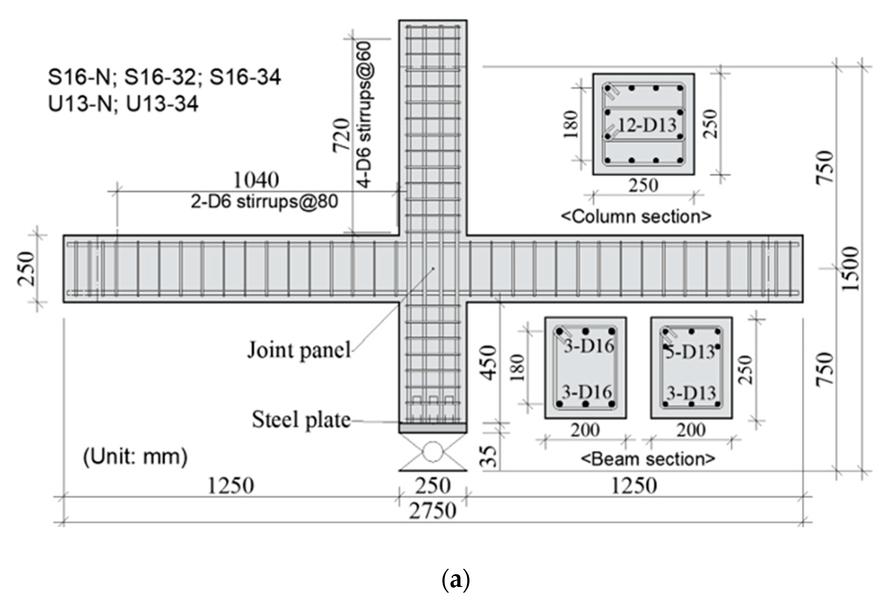
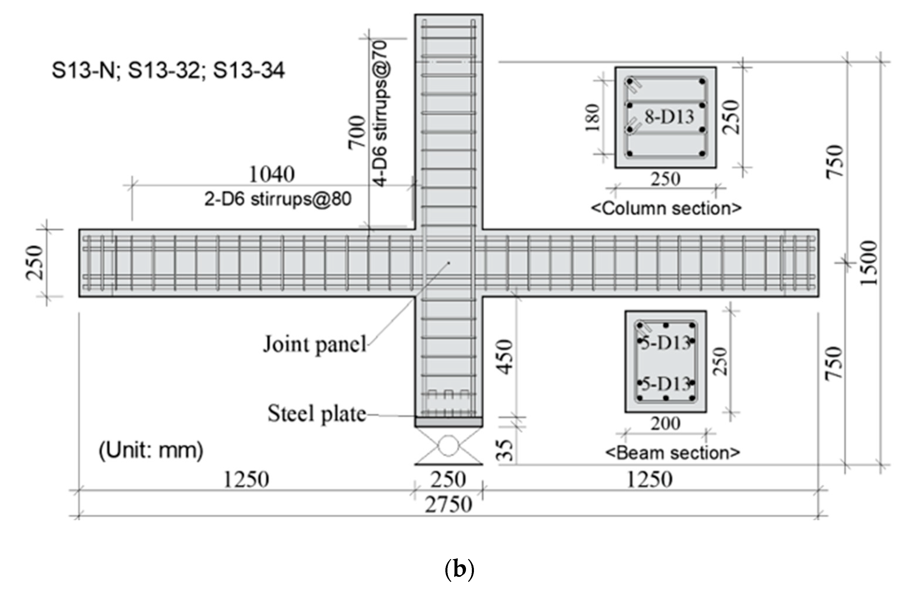
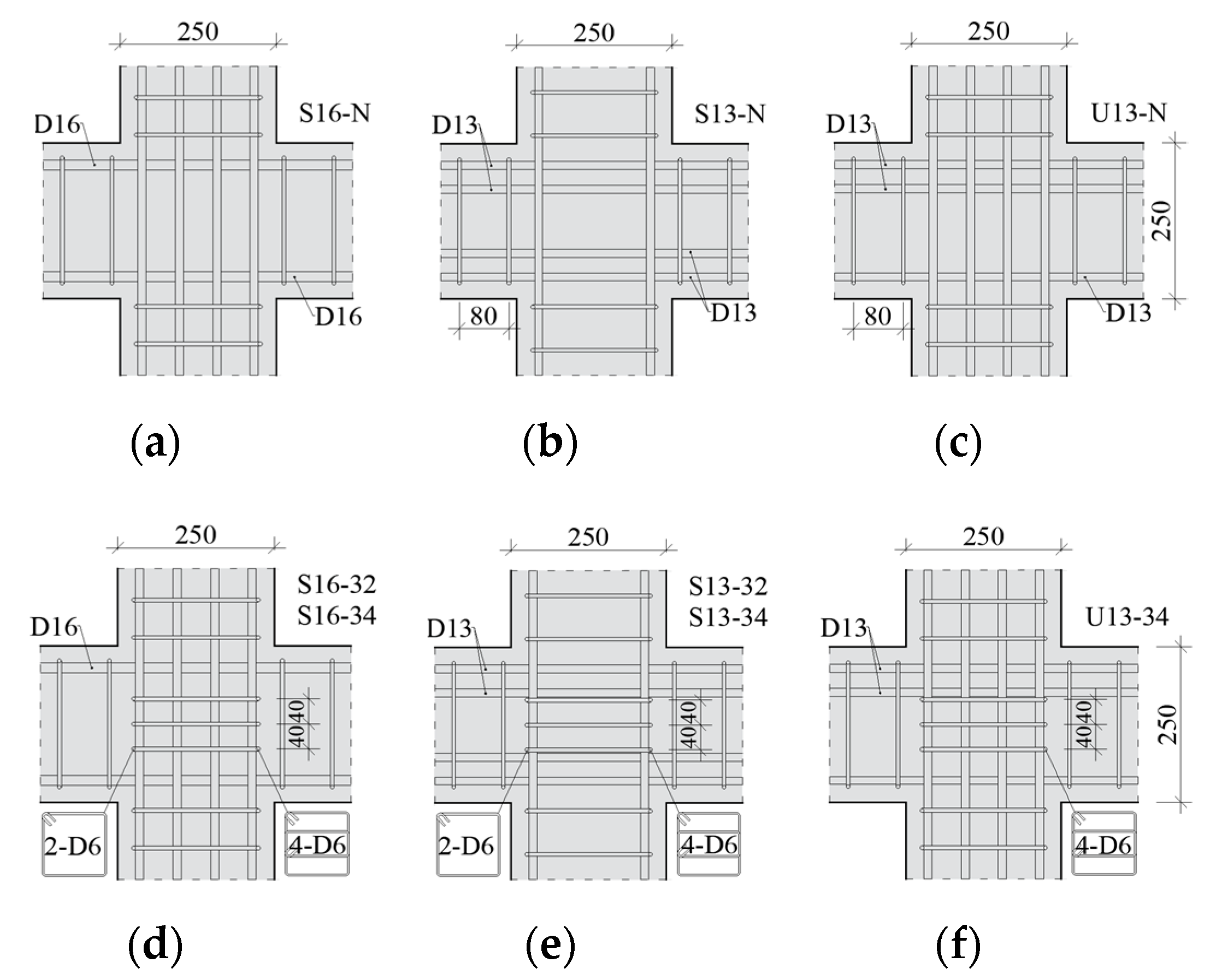
2.1. Test Specimens

Since there are less comprehensive test data available for the validation of the models, our test program has two main purposes: (1) to measure flexibility sources of RC interior beam–column joint sub-assemblages and gauge their relative contribution; and (2) to validate Shiohara’s hypothesis that “beam–column connections maintain shear strength during the lateral loading although joint shear deformation increases and lateral load degrades.” Eight interior joints were tested under cyclic lateral loading. The test specimens were half-scale models, representing beam–column sub-assemblages of a typical perimeter moment-resisting RC frame. The specimens were divided into three groups. The specimens in Group 1 were labeled as S16-N, S16-32, and S16-34, and the labels S13-N, S13-32, and S13-34 were assigned to the specimens in Group 2. Group 3 comprised two specimens: U13-N and U13-34. The specimen names indicate the test parameters. The numbers 32 and 34 at the end are the numbers of joint shear reinforcement layers with legs, and “N” indicates no shear reinforcement in the joint. “S” and “U” indicate symmetrically reinforced and unsymmetrically reinforced beams, respectively. The numbers 13 and 16 indicate the diameters of the beam longitudinal reinforcement d b (in millimeters). The specimens were designed to have medium shear stress levels. The dimensions and reinforcement details of the specimens are shown in Figure 1, and the reinforcement details of the joint are presented in Figure 2.
The design parameters for each specimen are presented in Table 1. The joint reinforcement ratio ( ρ j = A s h / b c j ) ranged from 0 to 0.72%. A s h represents the total cross-sectional area of the joint shear reinforcement, including crossties, within a distance j between the top and bottom beam longitudinal reinforcing bars. b c represents the column width. The ratio of the column depth to the beam bar diameter was 15.6 for Group 1 and 19.23 for Groups 2 and 3. The cross-sectional dimensions of the columns and beams were 250 mm × 250 mm and 200 mm × 250 mm, respectively. The overall length of the beam was 2750 mm, and the net length between beam supports was 2500 mm. The total height of the column was 1500 mm (distance between the top and bottom reaction points). The hoops and stirrups of all the specimens had rectangular D6 deformed bars with a spacing of 60 and 80 mm for the columns and beams, respectively, to prevent the premature shear failure of the beams and columns. As shown in Table 1, the flexural strength ratio of the columns to the beams was in the range of 1.1–1.6. Thus, for all the test specimens, the beams were expected to yield before the columns. The joint shear demand and capacity were calculated according to ASCE 41 [15].

2.2. Material Properties

Concrete cylinders were tested. The average compression strength of the three cylinders was 27.5–28.6 MPa for Group 1 and 29.7–31 MPa for Group 2. The average concrete strength reached 32 MPa for Group 3. Concrete with a maximum coarse aggregate size of 15 mm was cast by setting the column parts of the specimens in the vertical direction. Table 2 presents the yield strengths f y and ultimate strengths f u of the reinforcing bars. A D6 bar was used for the shear reinforcements, and D13 and D16 bars were used for the longitudinal reinforcements of the beams and columns, respectively.

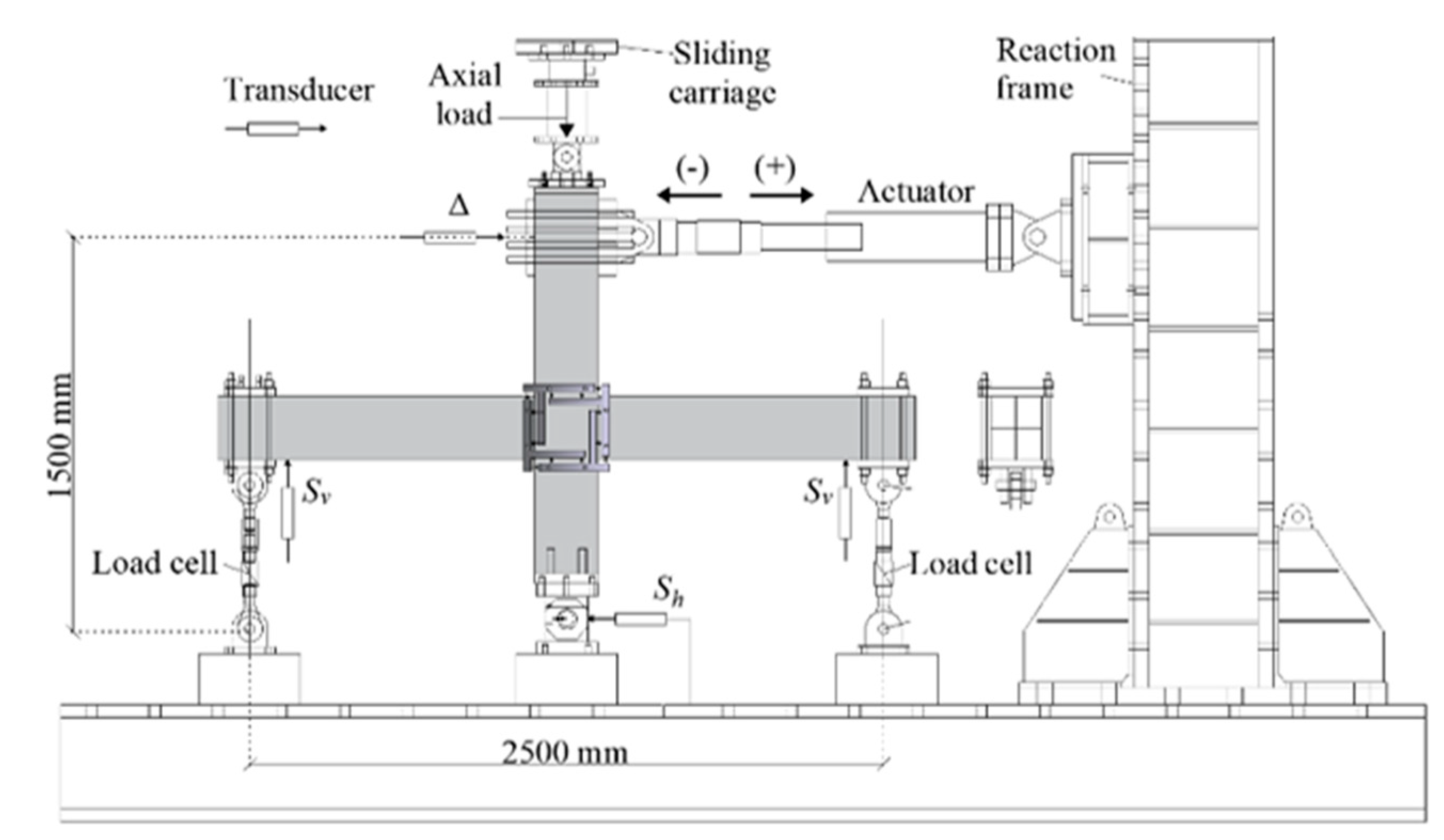
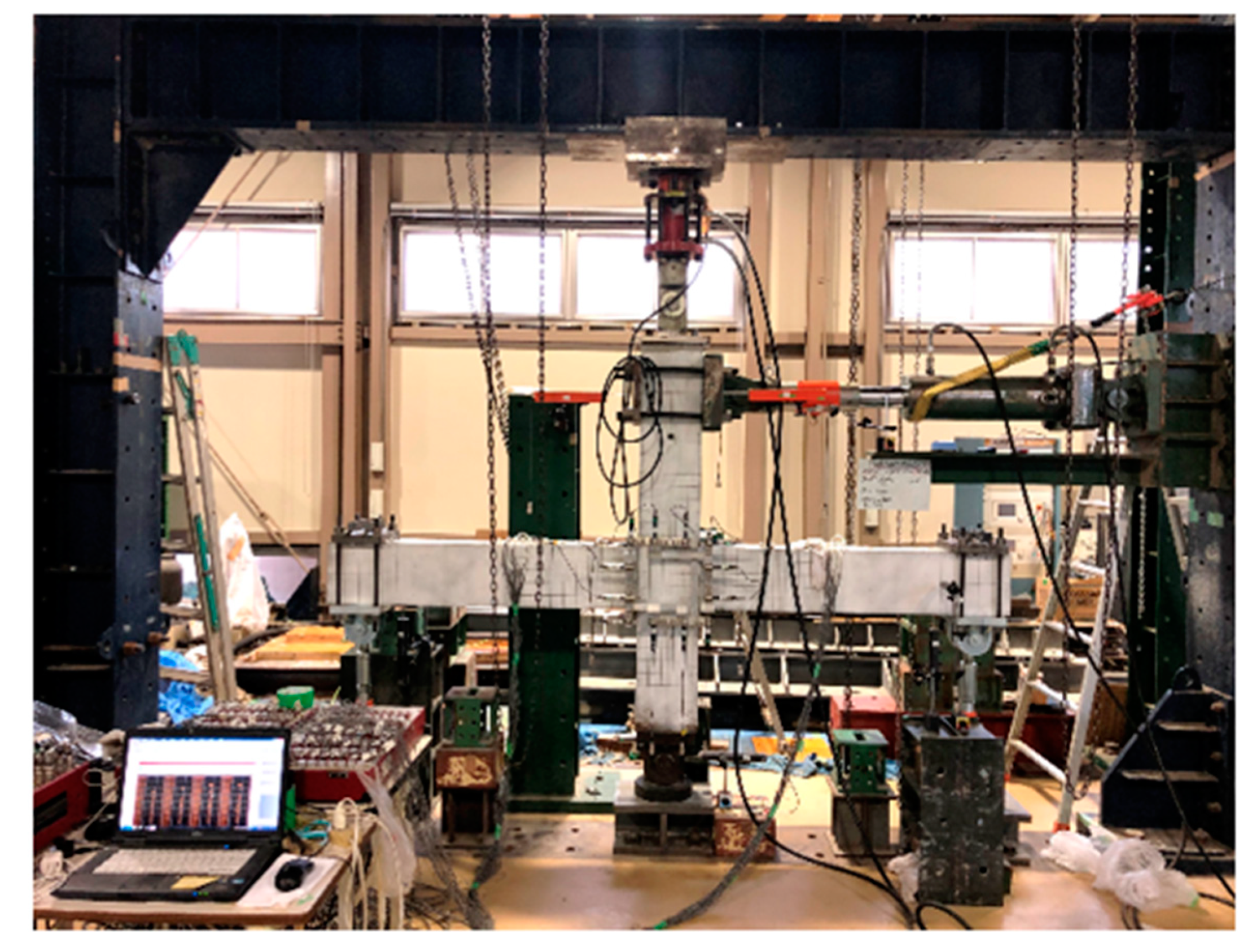
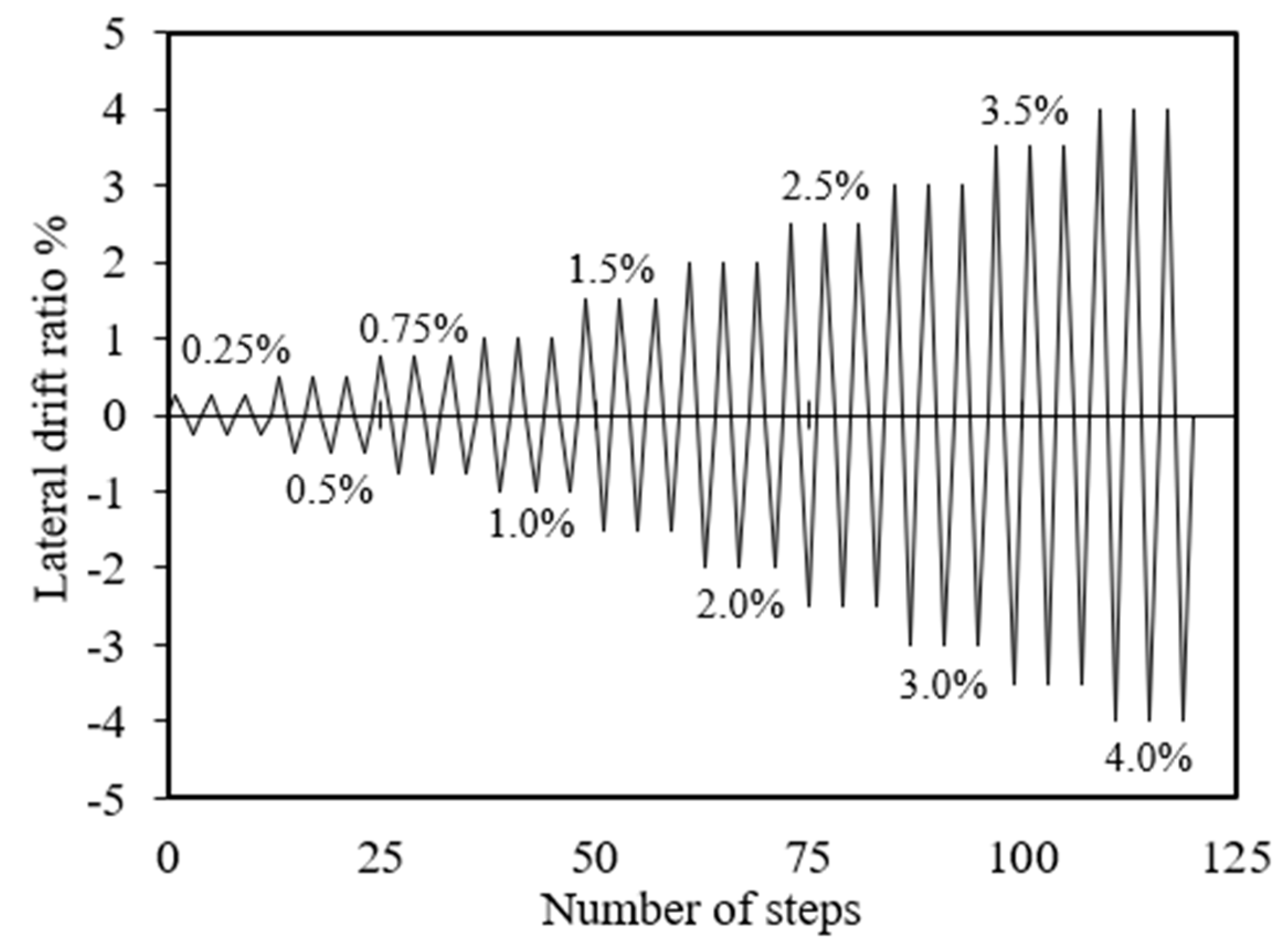
2.3. Test Setup and Loading History

Figure 3 shows the test setup of the interior beam–column joint. A photograph of the test setup is shown in Figure 4. A hinge support was used at the bottom of the column, and both ends of beams were roller supports to ensure that the beam would be free to move horizontally.
As reported by Park [27], quasi-static cyclic loading tests can be used to assess a toughness of the structure that would perform satisfactorily during a strong earthquake. Hence, quasi-static cyclic loading was employed in the test. The test was conducted under the displacement-controlled test method with the increasing of the lateral drift ratio. The lateral drift ratio is defined as the net lateral displacement divided by the net column height. The loading sequence is shown in Figure 5. It was planned by modifying the ACI 374.1-05 specifications [28]. At lateral drift ratios of 0.25%, 0.5%, 0.75%, and 1.0%, three loading cycles were applied. After the lateral drift ratio exceeded 1.0%, three loading cycles were applied at every 0.5% increase, and the cyclic loading was terminated when the load decreased to 50% of its peak value. The cyclic lateral load was applied to the top of the column. A constant vertical load with a magnitude of 0.1 f c A g was applied to all the specimens.

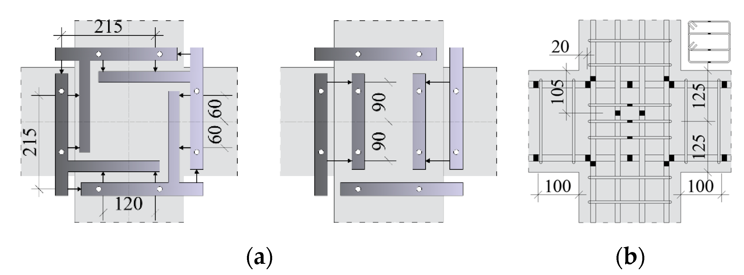
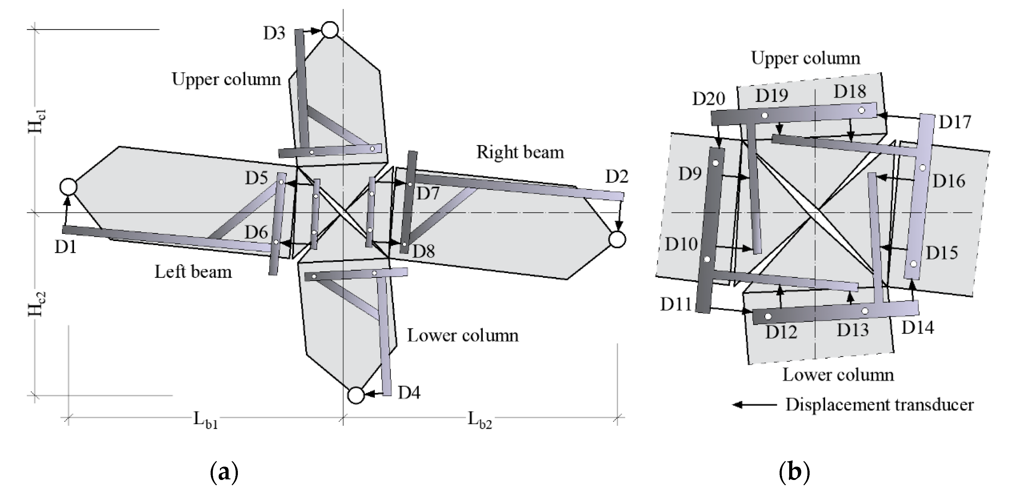
2.4. Instrumentation

Numerous strain gauges and linear variable displacement transducers (LVDTs) (Tokyo Measuring Instruments Lab, Tokyo, Japan) were installed on the test specimens to measure the strain at selected points on the reinforcing bars, as well as the deformations of different parts of the specimens. An instrumentation method recently proposed by Kusuhara and Shiohara [29] was adopted in this study. As shown in Figure 6a, 16 LVDTs were installed within the beam–column joint region to measure the components of the deformation of the beam–column joint, including the relative displacements of the member ends for three degrees of freedom as well as the components of the chord rotations of the beams and columns. The support movements ( S h and S v ) were monitored during the test to consider the effects of additional displacements on the lateral deformation of the specimens. The lateral load and displacement at the loading point were measured using the load cell in the actuator and an LVDT attached directly to the column, respectively. The reaction forces induced by the roller supports were measured using load cells throughout the test. Strain gauge locations on both longitudinal and transverse reinforcements within and around the joint region are illustrated in Figure 6b.
A mechanical motion of the measurement system for the deformation components of interior beam–column joint under inelastic deformation is illustrated in Figure 7. Shiohara [12,13] reported that the distribution of cracks and the associated damage pattern may be explained by considering the beam–column joint divided by into four rigid triangular parts rotating relative to each other. Unlike the assumption of uniform shear deformation over the joint region, shear deformation in the joint is assumed primarily due to the rotation of the four triangular concrete segments and the crack opening, as shown in Figure 7. Therefore, in order to obtain the joint deformation, the relative rotations of the assumed four segments were measured, and then, the measured data were converted to the subcomponents of the total deformation by referring to the previous study by Kusuhara and Shiohara [29]. The components of the total deformation ( R s ) proposed by Kusuhara and Shiohara are the lateral displacement due to chord rotations of beams and columns ( R s b and R s c ), fixed-end rotations of beams ( R s e ) , joint shear deformation ( R s p s ) , and rotations of faces of the beam–column joint ( R s p b and R s p c ).

3. Test Results

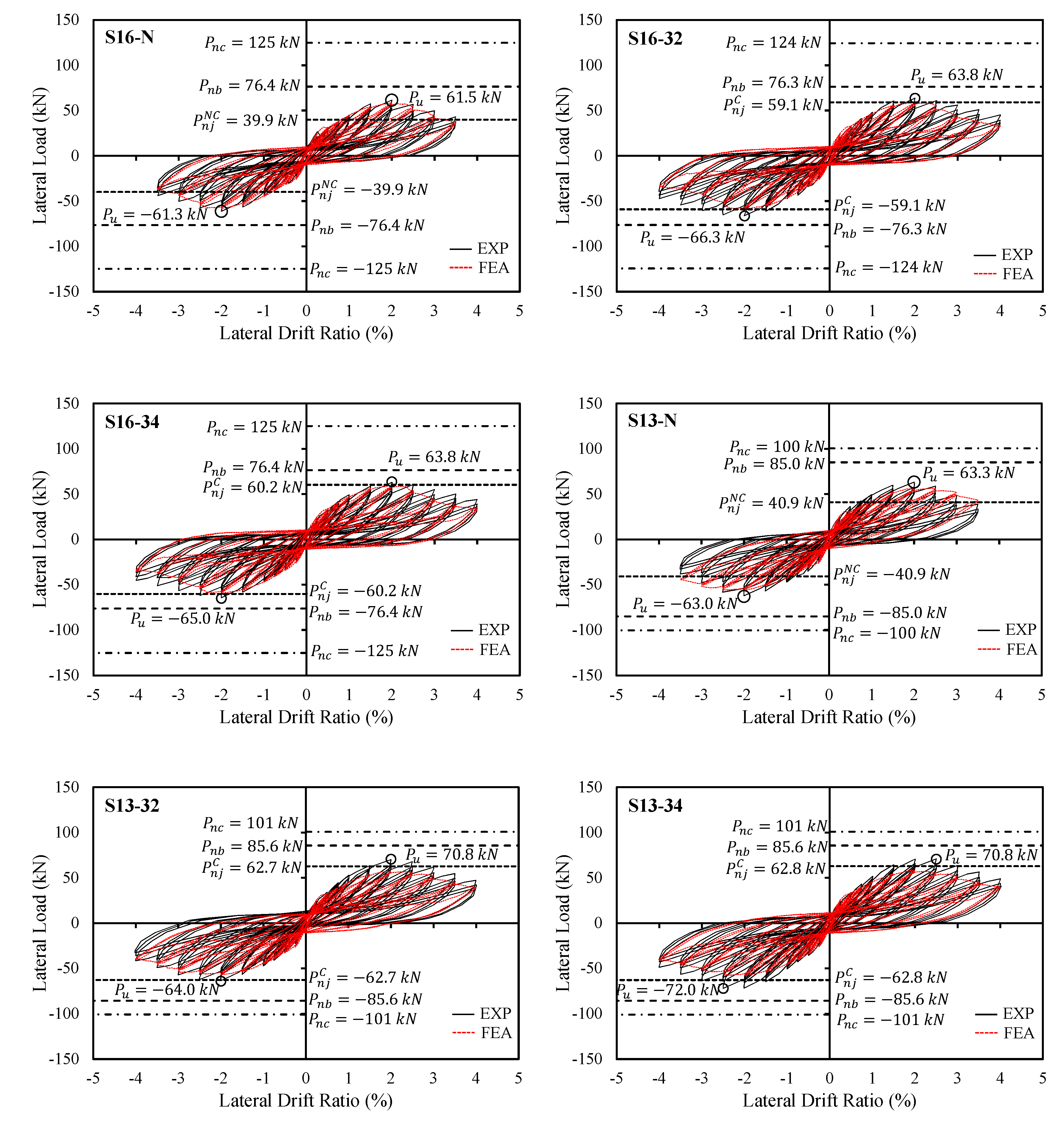
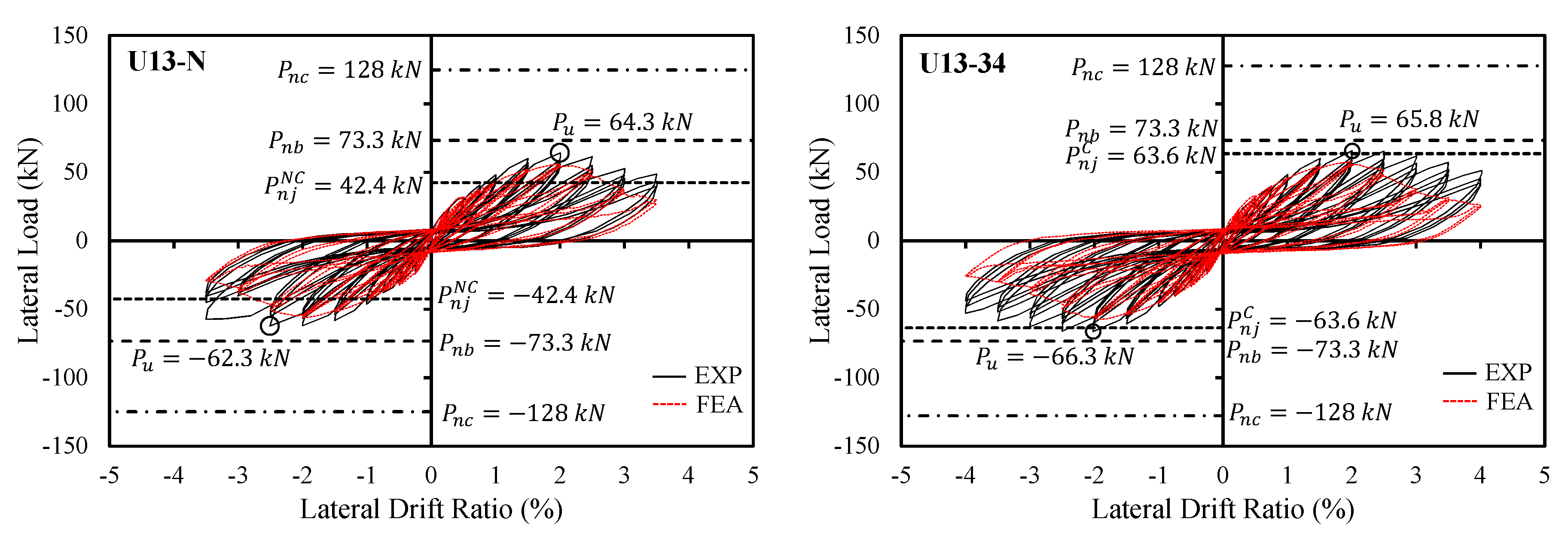
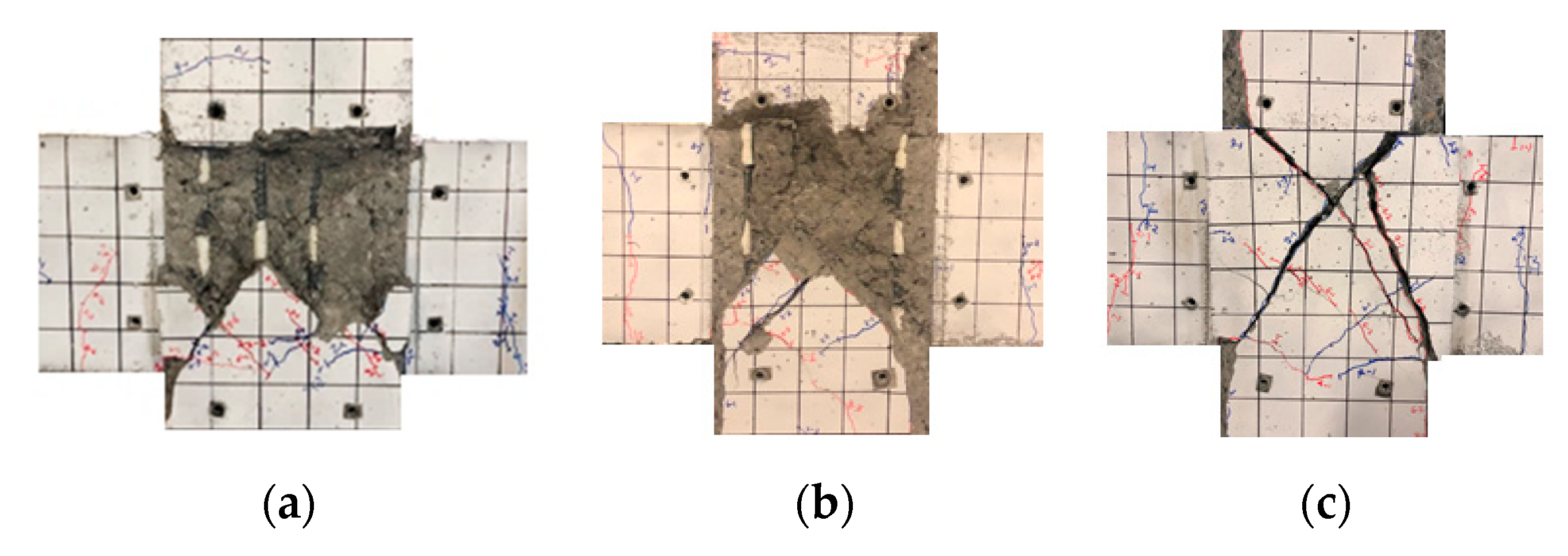
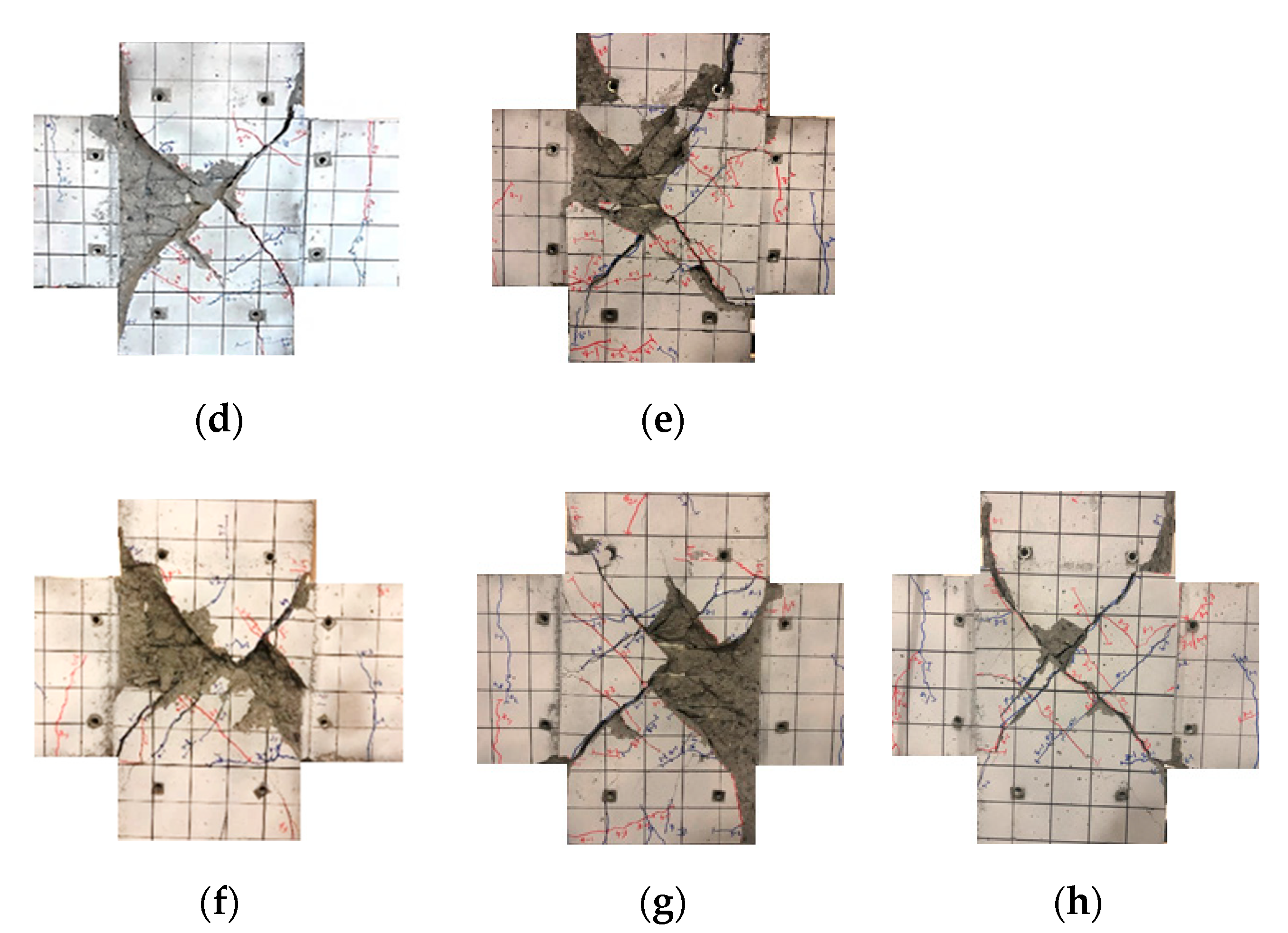
3.1. Lateral Load–Drift Ratio Relationships and Failure Modes

Figure 8 shows the hysteretic responses of the applied load ( P ) and drift ratio ( δ ) for the test specimens. The lateral drift ratio ( δ ) is defined as Δ n / H c . Here, Δ n represents the net lateral displacement at the loading point of the column without any support movements, and H c represents the column height (1500 mm). The circles in Figure 8 represent the maximum loads P u for the positive and negative lateral loadings. The horizontal dashed lines represent the theoretical lateral load-carrying capacities P n b , P n c , and P n j , which correspond to the beam yielding, column yielding, and joint shear failure, respectively. The detailed procedure for calculating these capacities is presented in Appendix A. Figure 9 depicts the failure modes of the specimens at the end of the test.
S16-N, S13-N, and U13-N (without joint shear reinforcement) reached the maximum loads at δ = 2.0 % . Subsequently, the strengths and stiffnesses gradually decreased, and the diagonal cracks in the joint began to widen (Figure 8). At δ = 3.0 % 3.5 % , the specimens exhibited joint failure owing to excessive cracking and spalling of the concrete (Figure 9a–c). Regarding the P δ relationship, the hysteresis loop became severely pinched, indicating lower energy dissipation. The average maximum loads, i.e., P u = 61.4, 63.2, and 63.3 kN for SRN16, SRN13, and URN13, respectively, exceeded the predicted joint shear strengths, i.e., P n j N C = 39.9, 40.9, and 42.4 kN, respectively. This indicates that ASCE 41 underestimated the joint shear strengths of the interior sub-assemblages ( ρ j = 0) by approximately 50.0%.
For S16–32 and S13–32 ( ρ j = 0.36), the overall hysteretic P δ relations and failure modes were similar to those of S16-34 and S13-34 ( ρ j = 0.72) (Figure 8 and Figure 9d–g). However, the maximum loads were increased to P u = 65.1 and 67.4 kN, respectively, compared with S16-N and S13-N. This was related to the joint shear reinforcement. The maximum loads of the specimens with the joint shear reinforcement were accurately predicted by ASCE 41.
In the cases of S16-34 ( P u = 64.4 kN) and S13-34 ( P u = 71.4 kN), the maximum loads P u were slightly larger than those of S16-32 and S13-32. Moreover, the specimens exhibited significant damage within the joint region with the concrete spalling despite the increased amount of the joint reinforcement (Figure 9f,g). Ultimately, joint failure occurred in S16–34 and S13−34. The maximum loads of P u = 64.4 and 71.4 kN for S16-34 and S13-34, respectively, were 7.0% and 13.0% greater than the joint shear strengths, i.e., P n j C = 60.2 and 62.8 kN, respectively (Figure 8).
For U13–34 (with ρ j   = 0.72 and the largest flexural strength ratio of 1.6), owing to the increased flexural strength ratio, the maximum load P u = 66.1 kN exceeded the predicted joint shear strength P n j C = 63.6 kN, and it was close to the beam yielding strength P n b = 73.3 kN. At δ = 3.0 % , gradual strength degradation occurred. Compared with the other specimens, the joint damage was significantly reduced, as shown in Figure 9h. The ultimate failure of this specimen was a joint failure, which occurred after the flexural yielding of the beam. The failure was comparatively ductile so that the specimen can be classified in the moderate ductility class according to ASCE 41. These results indicate that the joint shear reinforcement affected the lateral strength of the beam–column joint, which depended on the flexural strength ratio of the adjacent members.

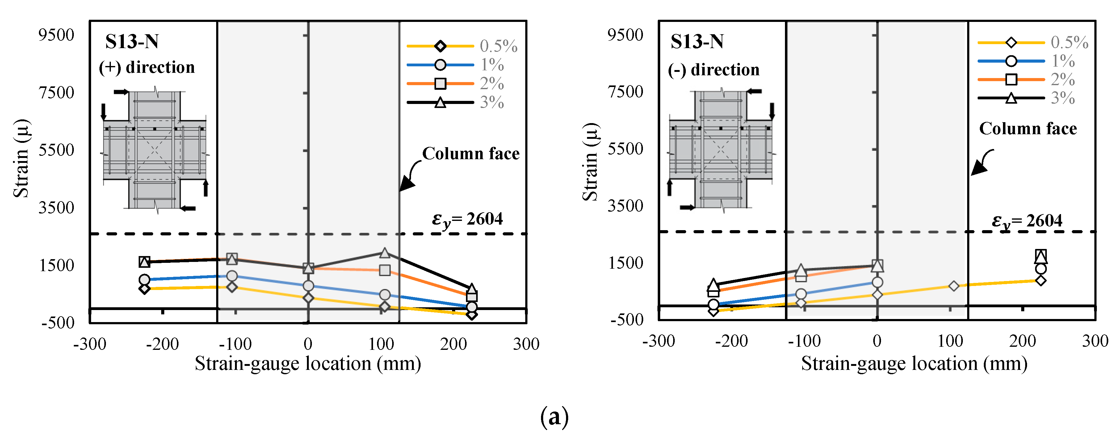
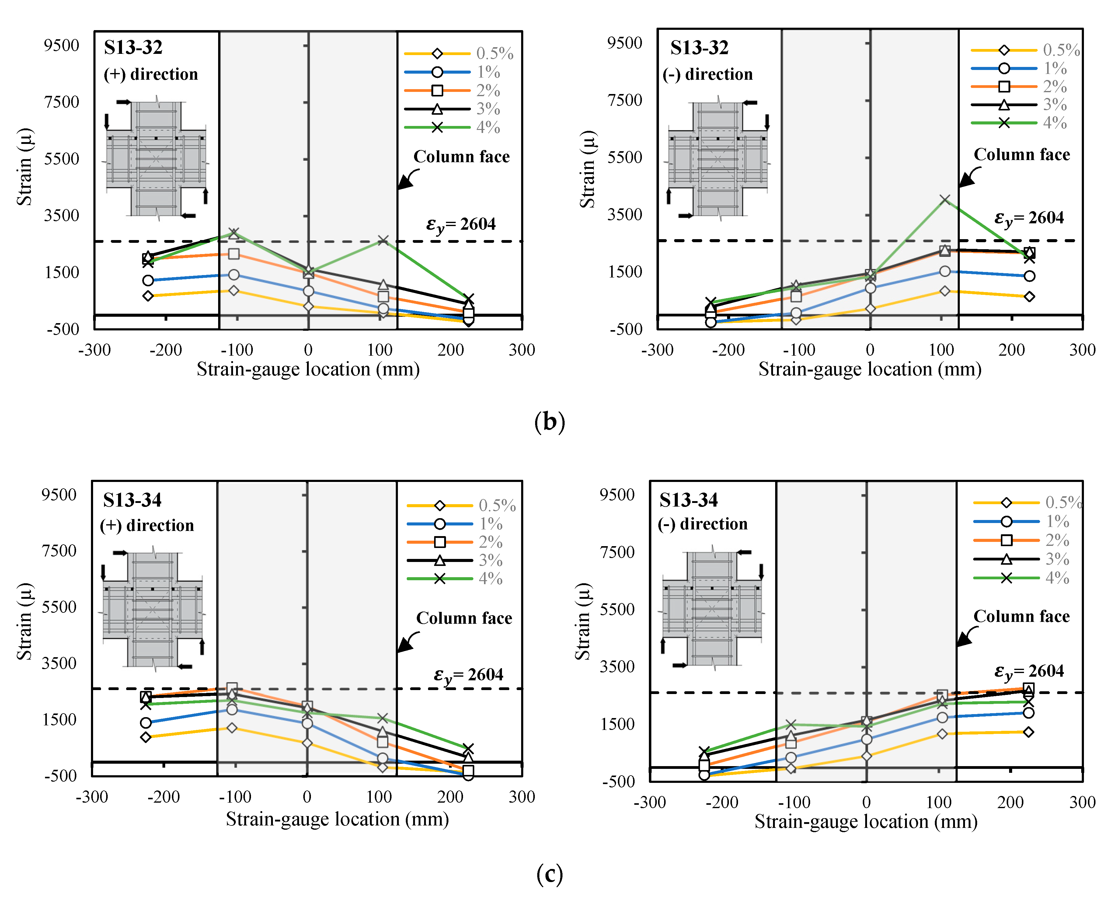
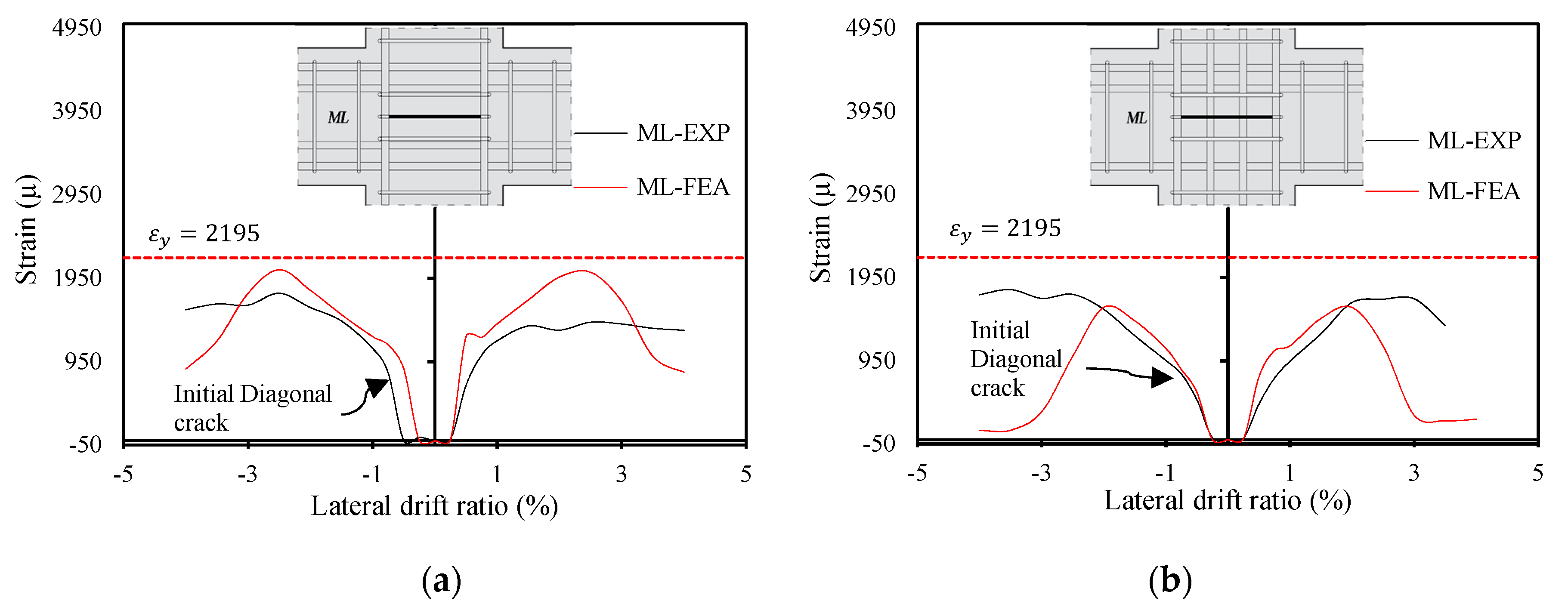
3.2. Strains of Beam Reinforcement

Figure 10 presents the strain developments of beam longitudinal reinforcements measured at the joint face and within the joint. The measured strain variations in the top beam bars were examined for S13-N, S13-32, and S13-34, which had the smallest flexural strength ratio of 1.1, to investigate the effects of the joint reinforcement on the shear stress and failure mode. Comparisons of the strain developments at the joint face and within the joint revealed the following.
  • At the peak strength of the specimens ( δ = 2.0 % ), the strains in flexural beam bars measured at the beam end (i.e., the joint face) were lower than the yield strains ( ε y t = 2604 μ) or equal to the yield strains. In the subsequent loading, the strains at the beam end did not increase. This indicates that the specimens failed owing to joint shear.
  • The amount of shear damage in the joint significantly decreased when the moderate amount of joint shear reinforcement was provided. Thus, the beam reinforcement strains at the beam end increased (compare the strains in Figure 10a–c). This indicates that the joint shear reinforcement successfully reduced the joint shear damage and increased the maximum lateral loads.
  • The beam reinforcement at the column right face under positive loading was subjected to compressive stress at the beginning of the test. However, above δ = 1.0 % , the bond deterioration of the beam-reinforcing bar passing through the joint occurred. Consequently, the transition of the compressive stress in the beam bar on the compression side at the beam end section to the tensile stress occurred (Figure 10a–c). The concrete took this compressive stress in the beam bar on the compression side, and the height of the compressive zone for the concrete may have increased, resulting in a smaller moment of the lever arm. Therefore, the moment in the beam section at the column face may have decreased. This phenomenon may have caused lateral strength degradation and stiffness degradation in all the test specimens (Figure 8). Our experiments are consistent with previous findings in the literature (Hakuto et al. [5] and Shiohara [12]).

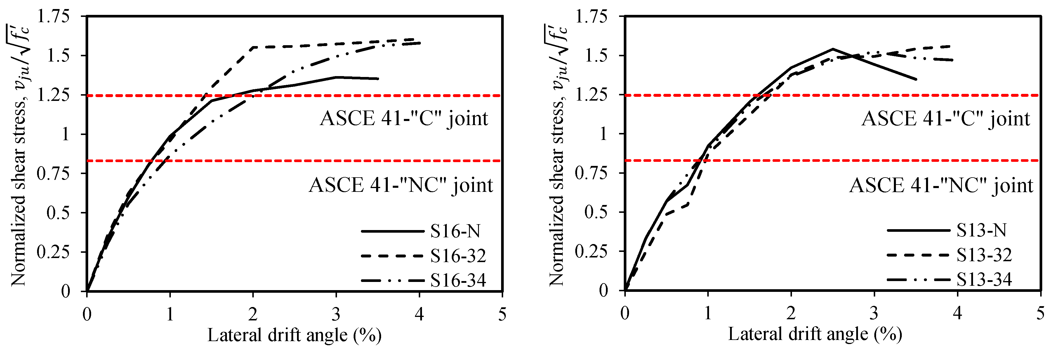
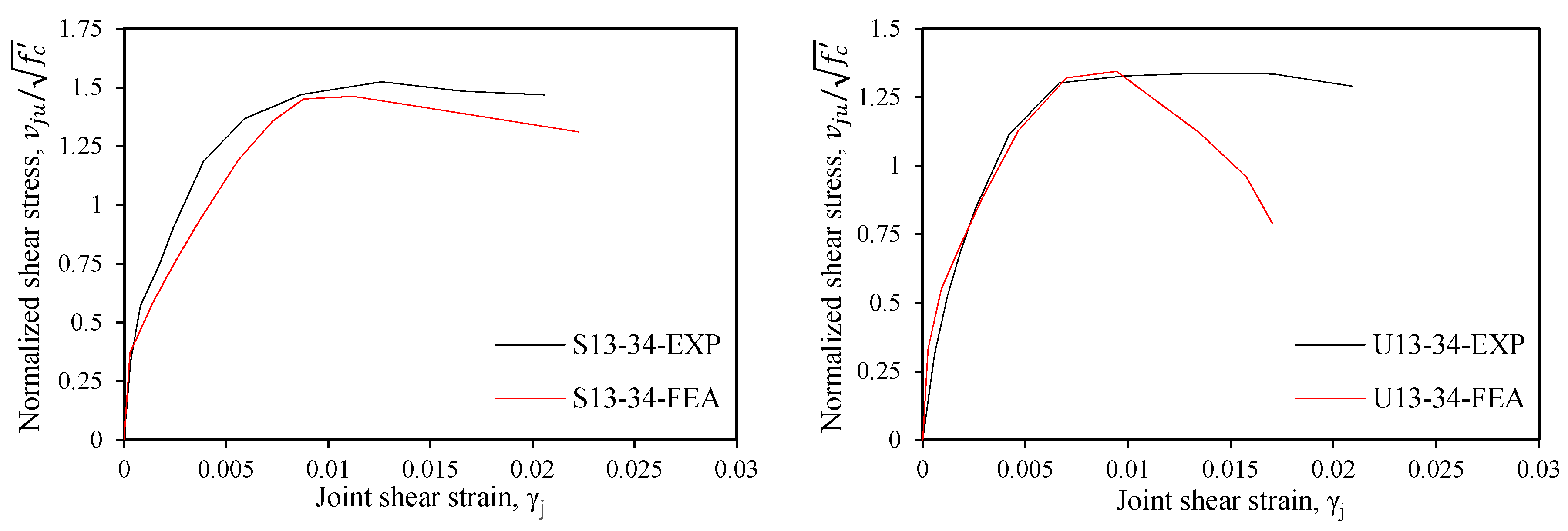
3.3. Joint Shear Stress

The joint shear stresses of the six specimens at the lateral load peaks in each loading cycle were plotted with respect to the lateral drift angle, as shown in Figure 11. For all the specimens, the strains in the reinforcements of the beam were measured and monitored during the test. The joint shear ( V j ) was calculated via Equation (A4) using the measured strain values, and the joint shear stresses were calculated using Equation (1). Since the strain of only one rebar was measured in the case of the beam bottom layer, it was assumed that the stresses were identical for all the bars belonging to the same layer.
v j = V j A j ;   V j = T b r + T b l P
Here, A j represents the effective joint area, which was used for the calculation of the joint shear stress and was a product of the column depth ( h c ) and the effective joint width b e = ( b c + b b ) / 2 , where b c and b b represent the widths of the column and beam, respectively. The calculation of the effective joint width was different from the ACI 352 recommendations [30], where the effective joint width b e is taken as M i n   [ b c ; b b + 0.5 D c ]   i f   b c > b b . The joint shear stress was normalized by the square root of the concrete compressive strength.
The maximum shear stresses, v j = 1.36 f c , 1.54 f c , and 1.32 f c MPa for nonconforming joints S16-N, S13-N, and U13-N, significantly exceeded the predicted joint shear strength v j n = 0.83 f c MPa. In the cases of S16-32, S16-34, S13-32, S13-34, and U13-34 (conforming joint), the maximum shear stresses v j were greater than those of S16-N, S13-N, and U13-N owing to the joint shear reinforcement. Nevertheless, the specimens displayed significant damage within the joint region with the spalling of cover concrete. The attained maximum shear stresses of the specimens with the joint shear reinforcement were greater than the ASCE 41 predictions. This indicates that the ASCE 41 shear limits for joint shear are conservative for nonconforming and conforming interior joints under certain combinations of design parameters.
In contrast to the results in Figure 8, the joint shear stress increased monotonically with the increasing lateral drift ratio for S16-N, S16-32, S13-32, and S13-34 (except for S13-N). For the specimens with the joint shear reinforcement, the joint shear stress and the width of the diagonal cracks on the joint core surfaces increased as the lateral drift increased. For all the specimens, approximately 40.0% of the total lateral drift was caused by the joint shear deformation at the maximum shear stress v j , and the corresponding lateral drift ratio was approximately 3.0–3.5%. Thus, the widening of the diagonal cracks and degradation of the lateral load-carrying capacity at a larger lateral drift ratio did not result from the degradation of the joint shear strength. Furthermore, the results indicate that the joint shear stress was not proportional to the lateral load P . Accordingly, the “joint shear” is a useful index for the beam–column joints with heavily reinforced beams (i.e., high shear stress levels), but it is unsuitable for defining the shear failure of beam–column joints with moderately reinforced beams (i.e., medium shear stress levels). Hence, the consideration of joint distortion corresponding to the shear stress is vital for the joints.

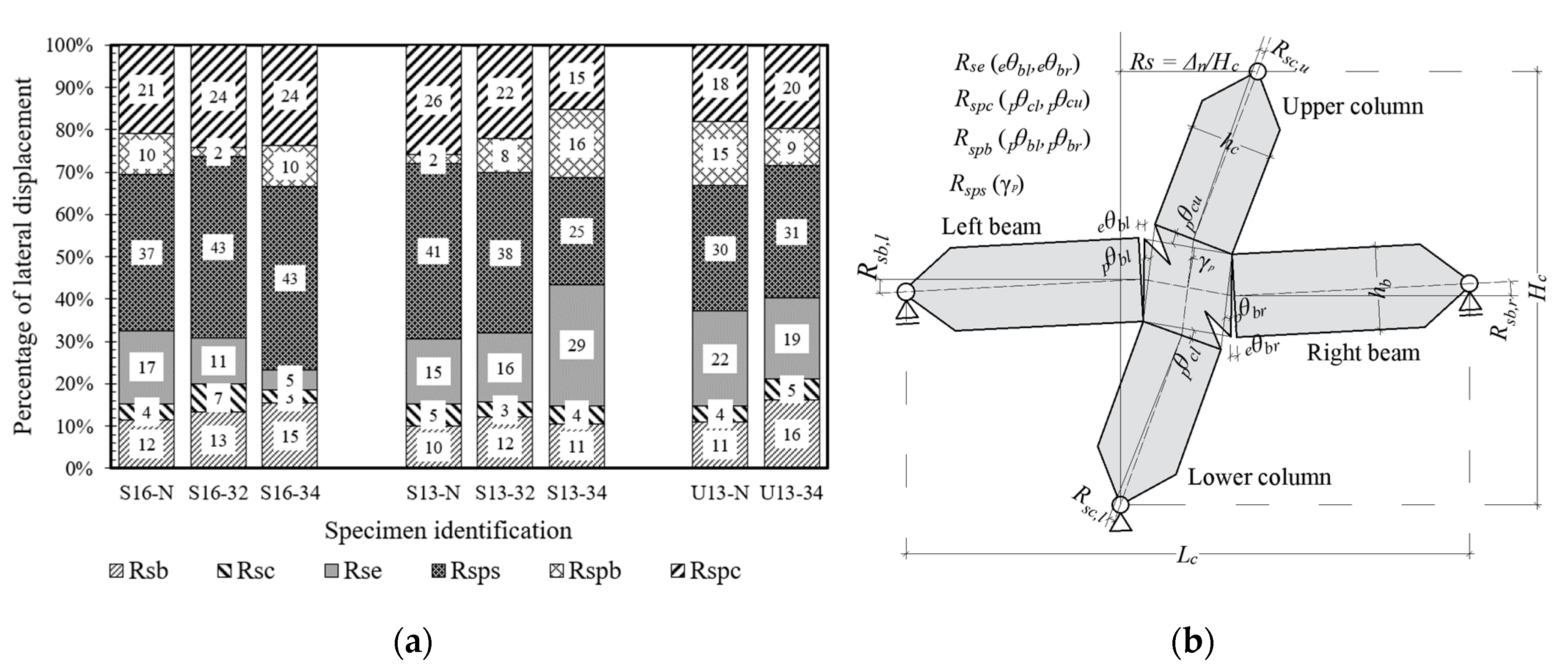
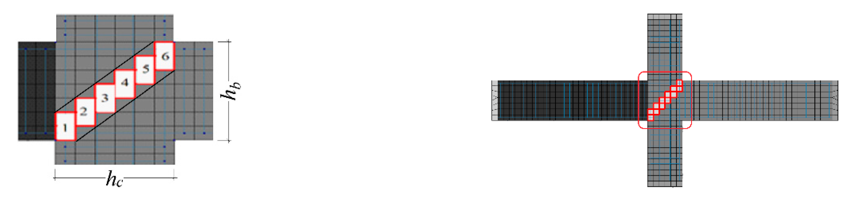
3.4. Decomposition of Lateral Drift

Percentages of decomposition of the total lateral drift measured at the top of the column at δ = 3.5% and the deformation components are shown in Figure 12. The components of the total deformation ( R s ) proposed by Kusuhara and Shiohara [29] are the lateral displacement due to chord rotations of beams and columns ( R s b and R s c ), fixed-end rotations of beams ( R s e ), joint shear deformation ( R s p s ) , and rotations of faces of the beam–column joint ( R s p b and R s p c ). These components were calculated using the procedure described in [29].
Lateral drift due to shear deformation ( R s p s ) and rotations of the faces of the beam–column joint ( R s p b and R s p c ) were dominant for all the specimens. This implies that the expansion of the joint at δ = 3.5% was significant for all the specimens. However, the shear deformation tended to decrease, owing to the shear reinforcement in the joint. For instance, the contribution of the shear deformation ( R s p s ) decreased by up to 25.0% for S13-34 ( M c / M b = 1.1), whereas the reduction was not significant for U13-34 ( M c / M b = 1.6). The lateral drift due to the chord rotations of the columns ( R s c ) accounted for only 3.0–7.0% of the total displacement for all the specimens. Similarly, the contribution of the lateral displacement from the chord rotations of beams ( R s b ) ranged from 10.0% to 16.0% for all the specimens. In contrast, the contribution of the beam fixed-end rotations to the total displacement ranged from 5.0% to 29.0% at δ = 3.5%. For Group 1, the fixed-end rotations decreased as the joint shear reinforcement increased. This is because the joint shear reinforcement improved the anchorage of beam reinforcement within the joint. Similar tendencies were observed in previous studies (Joh et al. [16] and Ichinose [7]). Our results for the lateral drift highlight the importance of considering the joint deformation since the primary source of the overall deformation of the specimens is joint deformation, which potentially causes a soft story mechanism [3,4].

4. Analytical Studies of Interior Beam–Column Joints

Due to a limited number of physical test specimens (a total of eight beam–column joints), no clear correlation was found between the test parameters and the failure mode of the joints. Hence, the results from the test program cannot be considered acceptable as the basis for drawing conclusions on this matter. To determine the relationship between the parameters identified in this study and joint deformation and/or failure mode, additional data on the cyclic behavior of RC interior beam–column joint connections for different combinations of the parameters are required. The nonlinear finite element (FE) analysis tool DIANA version 10.3 [31] was used for further investigating the complex behavior of interior joints. The validation and calibration of FE models were first done by simulating the experimental results to ensure that they will provide reliable predictions. Subsequently, the FE models were used to study the combined effects of the shear reinforcement ratio, flexural strength ratio, aspect ratio, and area ratio of adjoining members on the shear strength and shear deformation of interior beam–column joints.

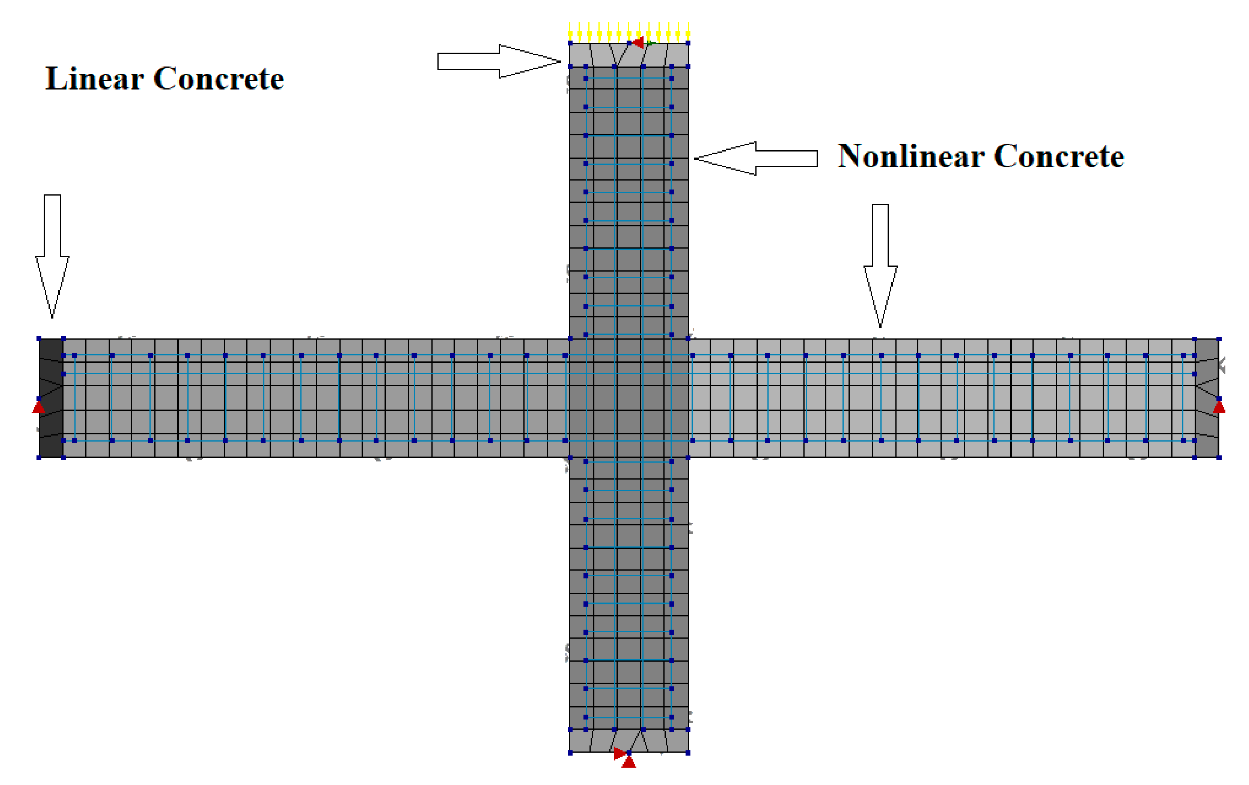
4.1. Finite-Element Modeling and Verification

In the FE analysis, two-dimensional continuum elements with quadratic interpolation of the displacement field were used for the concrete modeling, and the embedded steel reinforcement models were used for reinforcing bars. A total strain based rotating crack model was used in the analysis. Adequate tensile softening and compressive hardening–softening relations were considered, and the reduction of the concrete compressive strength due to lateral cracking was included. All reinforcing bars were assumed to be one-dimensional line elements with neither shear stiffness nor flexural rigidity. An elastic–plastic constitutive relationship with isotropic strain hardening was used to characterize the behavior of the reinforcement. All longitudinal reinforcing bars were connected to the concrete using the available interface elements in the DIANA library for accounting for nonlinear bond-slip. The bond–slip law used for the interface elements was based on the CEB-FIP model code 1990 [32]. The constitutive model and FE discretization are presented in Appendix B. The aforementioned FE modeling procedures and assumptions were determined by referring to a previous study performed by Deaton [33].
For verification, the FE analysis results were compared with the experimental results. The most common and often important comparisons are initial stiffness, capacity, deformation at peak load, and deformation at failure. Figure 8 presents the comparison between the hysteretic response of the test specimens in the experiment and the FE prediction. All those measures were successfully captured, and there was a satisfactory agreement between the experimental and analytical results. The comparisons were also made on the local behavior of the joints, including the strain developments of joint shear reinforcements and joint shear stress versus shear strain relations, as shown in Figure 13 and Figure 14. Although a complete agreement in the strain developments of the joint reinforcement for the test and analysis was not attained, it is seen that the strain values obtained from the analysis were similar to those observed in the test up to a drift ratio of 2.0%. Generally, FE models provided lower maximum loads than the test data, which explained the conservatism in the FE simulation. The maximum load estimated using the FE model was approximately 5.0–23.0% smaller than that observed in the test. The softening of the FE models after the maximum capacity was attained was similar to the test result; however, for some specimens, the FE models underestimated the post-peak behavior. Apart from those slight disagreements, the results confirmed that FE models could be used to predict the joint behavior by varying critical parameters.

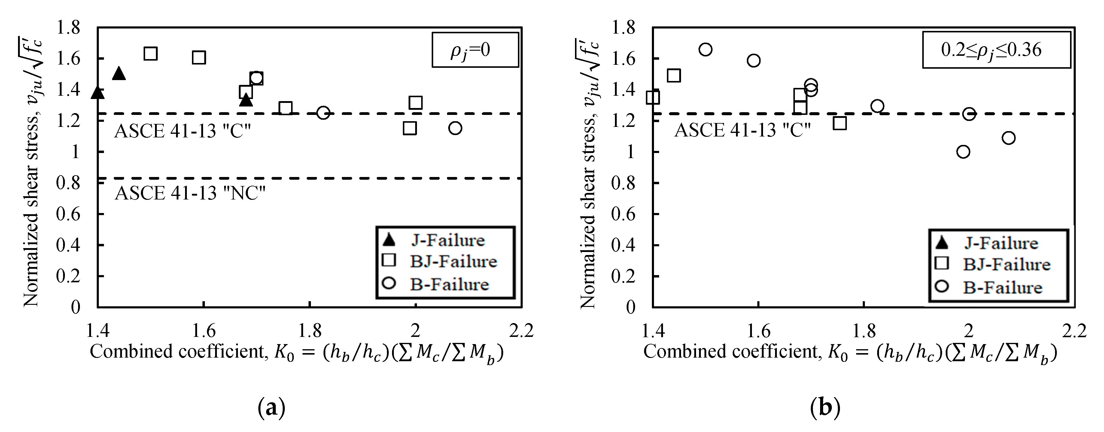
4.2. Parametric Studies

After the verification of the FE models against the experimental results, an extensive parametric investigation was performed to examine the shear stress and shear deformation of the interior beam–column joints and to develop simple equations to predict the joint shear deformation corresponding to three different failure modes without a comprehensive static or dynamic inelastic frame analysis. In the parametric study, 39 full-scale FE models were systematically constructed with varying parameters of design. The distance between the beam supports was 6000 mm. The total height of the column was 3000 mm. The cross-sectional dimensions of the columns were 500 × 500 mm2, 550 × 550 mm2, and 600 × 600 mm2, respectively. The following section presents the results of the parametric study. Additionally, the regression and correlation analysis were performed to investigate the relationship between the selected design parameters and joint shear behavior. Based on the analysis, three simple equations are proposed to predict the contribution of the joint deformation to the total deformation of beam–column joint connections.

4.3. Shear Stress and Shear Deformation of Interior Joints

Relative to the experimental results, ASCE 41 (Equation (A3)) was conservative in predicting the shear strength of both nonconforming and conforming joints for certain combinations of design parameters. Furthermore, ACI 352 specifies the joint shear strength with specific values of the design parameters, regardless of the deformation of the beam–column joints. Hence, the shear stress and shear deformation of the interior beam–column joints were investigated further, including the results of the parametric studies. The FE analysis results were compiled from the parametric studies. For all the FE models, the concrete compressive strength and compressive axial load level were set as constant values: f c = 28 MPa and N u / ( A g f c ) = 0.1. The ranges of the design parameters were 0 ρ j 0.72, 0.13 s / h c 1.0, 0.83 h b / h c 1.4, 1.0 M c / M b 2.5, and 0.89 A c / A b 1.8, respectively. The specimen properties and analysis variables are presented in Appendix C. According to the FE results, the failure types of 39 specimens were classified as follows: a joint failure after beam yielding was denoted as “BJ-Failure”, a joint failure prior to beam yielding was indicated as “J-Failure”, and a beam flexural failure was denoted as “B-Failure”. The maximum joint shear stress v j u was computed by averaging the shear stresses in diagonal elements of the joint panel in the FE models, and the same approach was applied to estimate the joint shear deformations (Figure 15).
Figure 16 shows the correlation between the normalized joint shear stress v j u / f c and design parameters. The joint shear reinforcement ratio, joint aspect ratio, and column-to-beam flexural strength ratio ( ρ j , h b / h c , and M c / M b , respectively) were considered as the parameters. In Figure 16a, for interior beam–column joints ( ρ j = 0), the range of v j u / f c was 1.15–1.63. However, some specimens exhibited B–Failure even if the v j u / f c was 30–70% greater than the ASCE 41 value for nonconforming joints.
The specimens with small joint reinforcement ratios ( ρ j ) of <0.36% exhibited large v j u / f c values of 1.0–1.65, as shown in Figure 16b. In this category, a few specimens exhibited BJ–Failure, whereas most of the specimens exhibited B–Failure. Figure 16c shows the normalized shear stress v j u / f c for specimens with moderate joint shear reinforcement ratios. The v j u / f c value was reduced by 7.0–39.0% for the specimens with larger values of the proposed coefficient K0, and all the specimens exhibited B–Failure.
The variation in the joint shear stress v j u / f c with respect to the proposed coefficient K0 is shown in Figure 16d. According to the results, joint failure did not occur even when the v j u / f c was relatively high. This means that joint failure does not always result from a lack of shear strength of the joint but rather insufficient moment resisting capacity. In that case, the joint shear deformation increases, although the joint maintains its shear strength. Thus, the joint acts similar to a hinge. The increase in the proposed coefficient K0, together with the joint shear reinforcement shifts the failure plane to a beam flexural hinge yield mechanism. This is because the moment resisting capacity of the joints increases with respect to the increasing amount of joint hoop and column-to-beam flexural strength ratio. These results are inconsistent with the ASCE 41 provisions for the shear-strength evaluation of interior joints, i.e., v j u = 0.83 f c for s > 0.5 h c and v j u = 1.245 f c for s 0.5 h c . Therefore, the “joint shear” is a useful index for the induced force level but is not suitable for defining joint failure. In addition to the joint shear index, it is necessary to consider the “shear deformation index” (SDI), which can be used to define the failure of beam–column connections.
The SDI versus the proposed combined coefficients K1 and K2 = ρj K1 is shown in Figure 17a–c for two expected structural deformations (in ASCE 41-13, the lateral story drift ratio of moment frames should be ≥4.0% for collapse prevention and 2.0% for life safety). The joint shear reinforcement ratio, area ratio of adjoining members, and column-to-beam flexural strength ratio ( ρ j , A c / A b , and M c / M b , respectively) were considered as the parameters. In this study, the structural deformations were assumed to be 3.5% for collapse prevention and 2.5% for life safety. Assuming that the joint deformation of the beam column joint contributes to the total lateral drift ratio, the SDI is defined as the ratio of the lateral drift ratio R s p s (Equation (2)) due to the joint deformation to the total lateral drift ratio R s .
R s p s = γ j ( 1 h c L b h b H c )
Here, γ j represents the joint shear deformation.
Although the combinations of the joint shear reinforcement ratio, joint aspect ratio, and column-to-beam flexural strength ratio ( ρ j , h b / h c , and M c / M b ) were considered as the parameters affecting the joint shear stress in Figure 16a–d, the area ratio of adjoining members was additionally included in terms of the joint shear deformation, instead of the joint aspect ratio. This is because the joint shear deformation exhibited a strong correlation with ρ j , A c / A b , and M c / M b . Therefore, the coefficients K1 and K2 = ρj K1 were proposed.
In all six figures, the contribution of the shear deformation to the total deformation of the beam–column joint connection decreases as the values of the proposed coefficients increase. According to the observed patterns, these graphs were classified into three categories depending on the SDI values. For instance, the first set of figures corresponds to a low ductility demand (<2), which is defined in ASCE 41. This is because the range of the SDI values was 0.4–0.8 at lateral drift ratios of 2.5% and 3.5% for specimens with ρ j = 0. This implies that heavy damage is expected in the joint region; thus, the main source of the overall deformation of a beam–column joint sub-assemblage is joint deformation. Consequently, the global displacement ductility of the sub-assemblage is reduced, which reduces the collapse-prevention capacity of the overall frame structure. The second set of graphs corresponds to a moderate ductility demand (2–4), and the third set of graphs corresponds to a high ductility demand (>4), as the SDI values ranged from 0.11 to 0.4 for the specimens with moderate joint reinforcement ratios. Based on these three groups of graphs, the following simple equations are proposed to predict the SDI of RC interior beam–column joint connections corresponding to three different failure modes: J-mode, BJ-mode, and B-mode. Each equation has its basic criteria for application. The graphical representations of the proposed equations are shown in Figure 18 Figure 19 and Figure 20.
The SDI corresponding to the J-mode (joint failure before beam yielding) can be expressed as follows:
SDI = 0.8 0 K 1 1 SDI = 0.8 K 1 0.6 1 K 1 3 .
Basic criteria for applying Equation (3):
  • M c / M b < 1.5
  • ( A s , t o p f y ) / ( b b d f c ) > 0.25
Regardless of the amount of joint hoop.
The SDI corresponding to the BJ-mode (joint failure after beam yielding) can be calculated by
{ SDI = 0.4 0 K 2 0.4 SDI = 0.3 K 2 0.3 0.4 K 2 2
Basic criteria for applying Equation (4):
  • 1.5 M c / M b < 2.0
  • 0.15 < ( A s , t o p f y ) / ( b b d f c ) 0.25
  • 0.25 % ρ j < 0.5 % .
The SDI corresponding to the B-mode (beam flexural failure) can be calculated using Equation (5).
{ SDI = 0.3 0 K 2 0.25 SDI = 0.15 K 2 0.6 0.25 K 2 4
Basic criteria for applying Equation (5):
  • 2.0 M c / M b < 3.0
  • 0.05 < ( A s , t o p f y ) / ( b b d f c ) 0.15
  • 0.5 % ρ j < 1.0 % .
Using Equation (3) to Equation (5), one can readily define the expected failure mode of beam–column joints and determine the contribution of the joint deformation to the total lateral drift of the system. These simple equations can be used for both the new design of interior joints and shear deformation evaluation of existing interior joints. It should be noted that for both cases, practicing structural engineers first need to calculate the flexural strengths of beams and columns, the area ratio of columns and beams, and the joint hoop ratio (if available) in order to determine which equation can be used for that particular situation.

4.4. Verification of Proposed Equations

The experimental shear deformation indexes (SDIs) of the tested eight specimens were compared with the SDI calculated using Equation (3), since the test specimens showed J-failure. Furthermore, to check the accuracy of the proposed equations, 50 available experimental results reported in the previous investigations were compared with the SDI values predicted by the equations. The ranges of the experimental database were 21 f c 107 , 0 N u / ( A g f c ) 0.3 , 0 ρ j 1.6 % , 0.89 h b / h c 1.67 , 0.88 M c / M b 5.15 , 0.03 ( A s , t o p f y ) / ( b b d f c ) 0.5 , and 0.6 A c / A b 1.58 , respectively. Out of 50 specimens, 15 specimens were reported to show J-type failure, and 16 specimens exhibited BJ-type failure. Nineteen specimens failed due to beam flexure (B-type failure). The specimen properties and analysis variables are presented in Appendix D.
The accuracy of the proposed equations is gauged in terms of a shear deformation index (SDI) ratio, which is defined as the ratio of the measured SDI to the predicted SDI. The SDI ratio of 1 indicates perfect accuracy; the SDI ratio > 1 indicates that the equations tend to be conservative; and the SDI ratio < 1 suggests that it is non-conservative. Figure 21 shows a comparison between the measured and predicted SDI values. Equation (3), Equation (4), and Equation (5) predict the SDI values of the existing test results with respective mean values of 1.03, 0.89, and 0.76 for the SDI ratio and corresponding coefficients of variation (COVs) of 18.0%, 14.0%, and 35.0%. Although there was a low correlation between measured and calculated SDI values for Equation (5), it was proved that the predictions of Equation (5) were on the safe side. By comparing the results of Equation (3), Equation (4), and Equation (5) with experimental results, it was concluded that the proposed equations have reasonable accuracy. The relative ease of the calculations and the accuracy of the results indicate that the proposed equations would be suitable for routine design by practicing structural engineers. In addition, the SDI prediction is considered useful for the displacement-based design of moment frames, which are significantly affected by joint damage.

5. Conclusions

Three equations were proposed in this study to predict the joint shear deformation index (SDI) of RC interior beam–column connections corresponding to three different types of failure (i.e., joint failure before beam yielding, joint failure after beam yielding, and beam flexural failure). To develop such equations, experimental and analytical studies were conducted on eight half-scale joint specimens and 39 full-scale FE models of beam–column connections with various combinations of joint design parameters. The SDI values of 50 beam–column joints reported in the literature were compared with those predicted by the proposed equations to validate their applicability. According to these investigations, the following conclusions are drawn.
  • With regard to the strength and stiffness, the performance of the test specimens was satisfactory up to δ = 2.0% (lateral drift ratio), beyond which the strength and stiffness generally degraded. The maximum loads occurred at δ = 2.0–2.5%, after which concrete cracking and spalling became severe at δ = 3.5–4.0%. Among the eight specimens, S13-N exhibited the worst performance. This was mainly due to the absence of joint shear reinforcement and the smaller flexural strength ratio.
  • Experimental and finite-element investigations indicated that throughout the lateral loading, the joint shear stress increased, while the width of the diagonal shear cracks on the joint core surfaces increased. The maximum joint shear stress values exceeded the limits of v j u = 0.83 f c for s > 0.5 h c and v j u = 1.245 f c for s 0.5 h c suggested by ASCE 41. The joint shear deformation contributed approximately 40% of the total lateral drift at the maximum shear stress v j , and the corresponding lateral drift ratio was approximately 3.0–3.5%. This indicates that the “joint shear” is a useful index for the beam–column joints with high shear stress levels of v j 1.7   f c but is unsuitable for defining the shear failure of beam–column joints with medium or low shear stress levels of v j 1.25 1.5 f c and v j 1.0 f c .
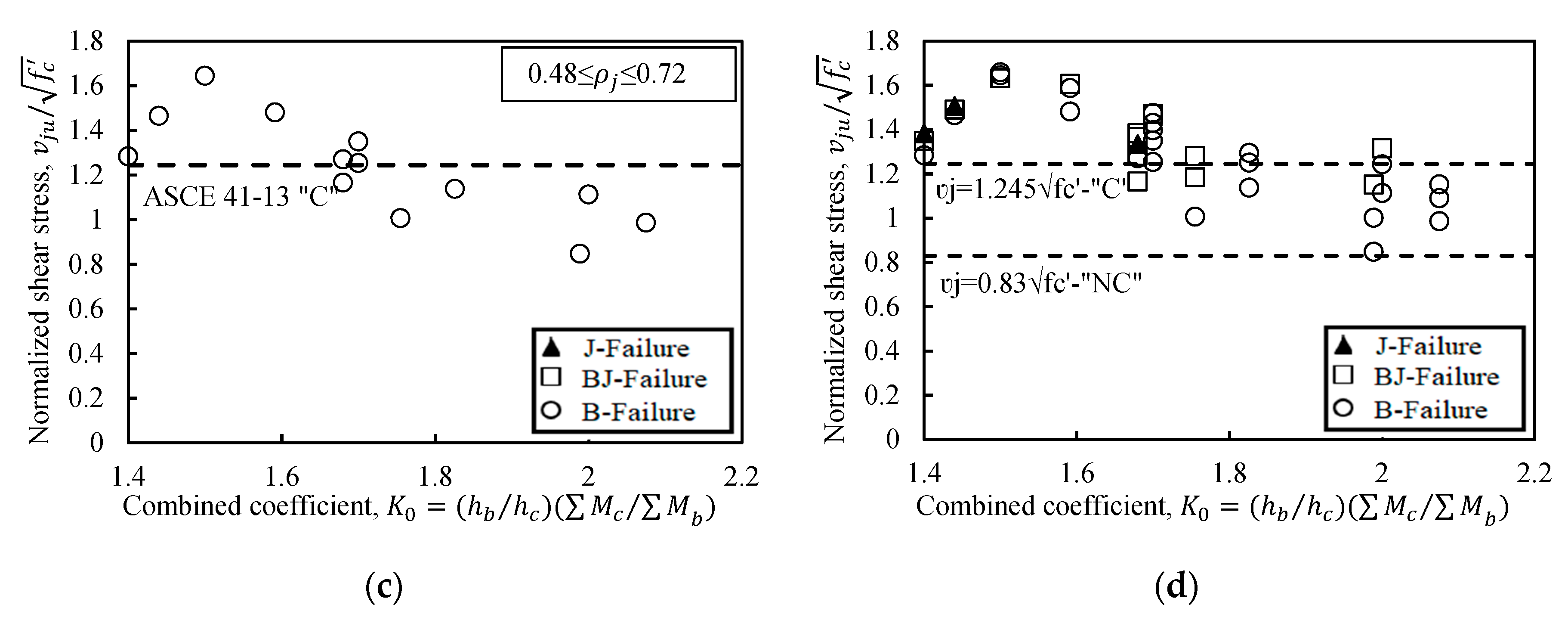
  • Using the results of parametric studies (39 specimens), the shear stress of the interior joints was investigated considering the design variables ρ j , h b / h c , and M c / M b . The maximum shear stress v j u varied between 0.85 f c and 1.65 f c . However, joint failure did not occur in some specimens, even if v j u / f c was relatively large. This is because the increase in the proposed coefficient K0, together with the joint shear reinforcement shifts the failure plane to a beam flexural hinge yield mechanism.
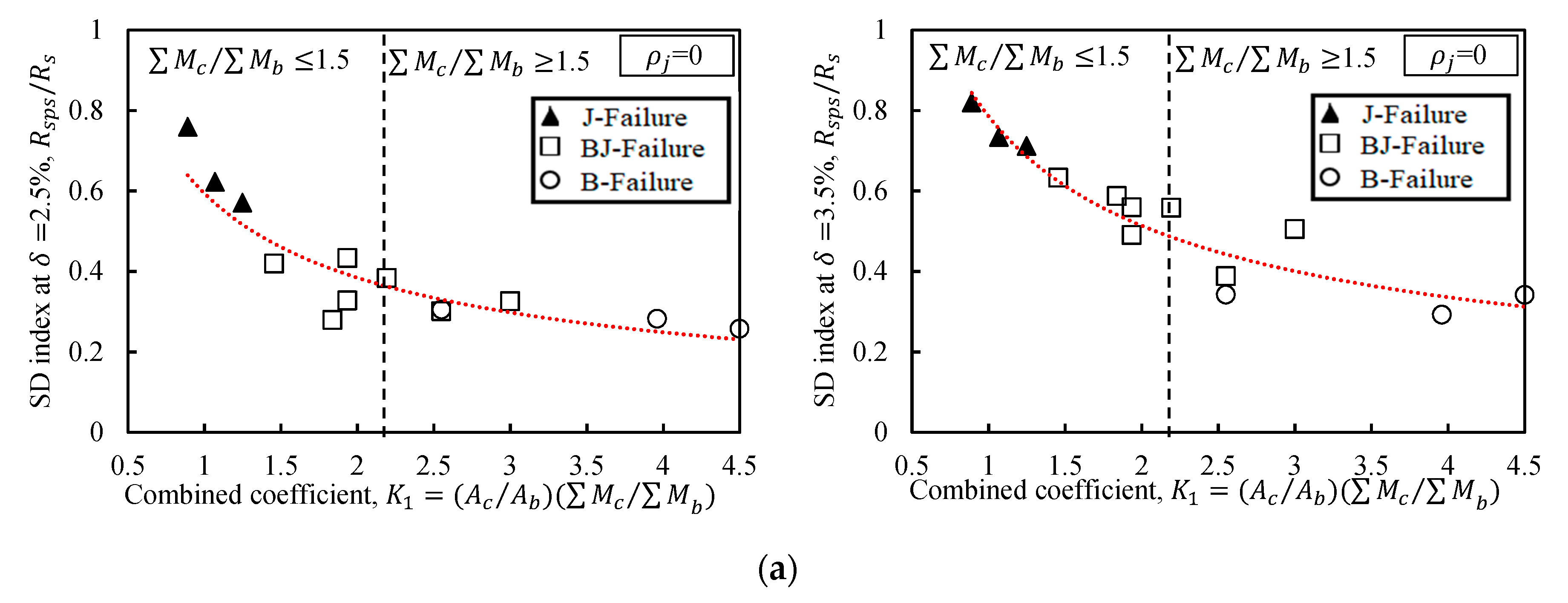
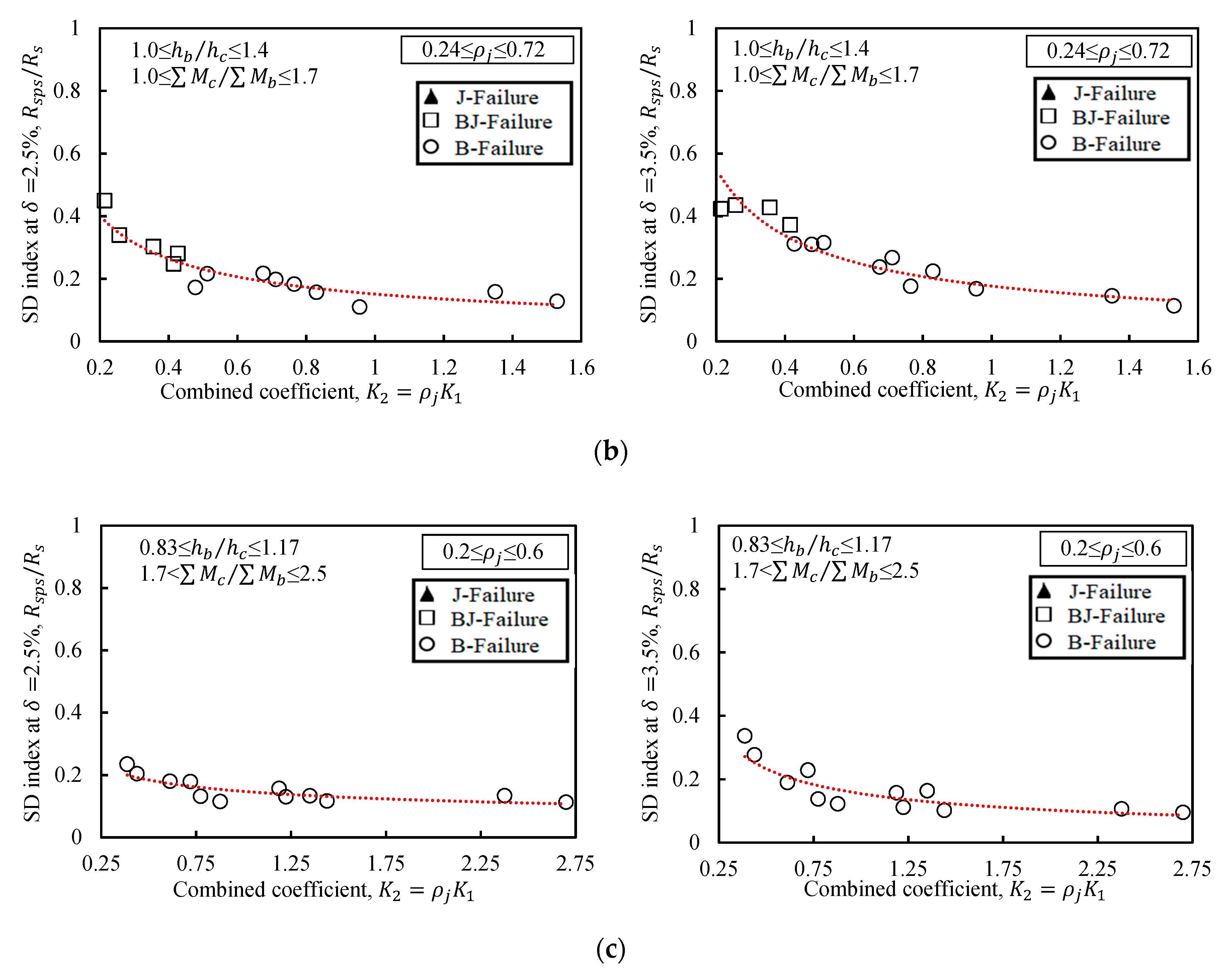
  • The shear deformation of interior joints was examined with consideration of the design variables ρ j , A c / A b and M c / M b . The contribution of the joint shear deformation to the total deformation ranged from 10.0% to 80.0% depending on the values of the proposed coefficients K 1 and K 2 = ρ j K 1 . The joints with smaller values of K 1 and K 2 performed poorly, exhibiting wide inclined cracks and deformations that accounted for up to 80% of the overall lateral deformation ( δ = 2.5% and δ = 3.5%). Larger values of K 1 and K 2 yielded smaller deformation of the joint region.
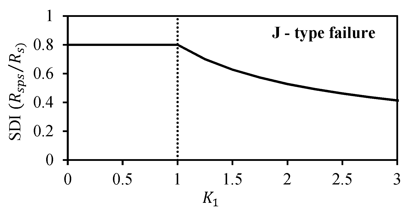
  • The design based on limiting the joint shear stress can be used for safety. However, it should be supplemented with consideration of the corresponding joint shear deformation to define the joint failure clearly. According to the results, three simple equations were proposed for predicting the joint deformation contribution to the total story drift of beam–column joints under critical structural deformations. The equations were able to predict SDI values with reasonable agreement with the experimental data. Compared with previously proposed models and theories, our method does not require complex nonlinear numerical analyses of the structure or sub-assemblage.

Author Contributions

Analysis, investigation, data curation, and writing—original draft preparation, D.G.; supervision, writing—review & editing, and software, T.M. All authors have read and agreed to the published version of the manuscript.

Funding

This research received no external funding.

Conflicts of Interest

The authors declare that there is no conflict of interest.

Appendix A. Current Design Methods

For interior beam–column connections, the following three failure modes are considered: (1) flexural yielding of the beam or column, (2) shear failure of the joint, and (3) bond failure of the longitudinal beam reinforcement. The lateral forces corresponding to each failure mode can be estimated as follows.

Appendix A.1. Flexural Yielding of Beam or Column

Figure A1 shows the support reactions ( V c , V b r , and V b l ) and internal moments at the joint face ( M c , M b r , and M b l ) in an interior beam–column connection specimen subjected to a lateral load ( P ) at the top of the column. When yielding of the column occurs before yielding of the beam (in the case of a low-rise building), the lateral force ( P n c ) based on column yielding is given as
P n c = M c ( H c h b ) / 2 = 2 M n c H c h b
where M n c represents the nominal flexural strength of the column, and H c represents the distance from the bottom support of the column to the loading point. (For actual columns, H c represents the distance between the inflection points in the upper and lower columns.)
Figure A1. Internal forces and reaction forces acting on an interior beam–column connection under a lateral load.
Buildings 10 00176 g0a1
When yielding of the beam occurs, the corresponding lateral force P n b can be calculated from the moment equilibrium (Figure A1):
P n b = ( V b l + V b r ) L b 2 H c = ( M n , b l + M n , b r ) L b H c ( L b h c )
where M n , b l represents the nominal flexural strength of the beam, and L b represents the distance from the left beam support to the right beam support. (For an actual beam, L b represents the distance between two inflection points of the beam.)

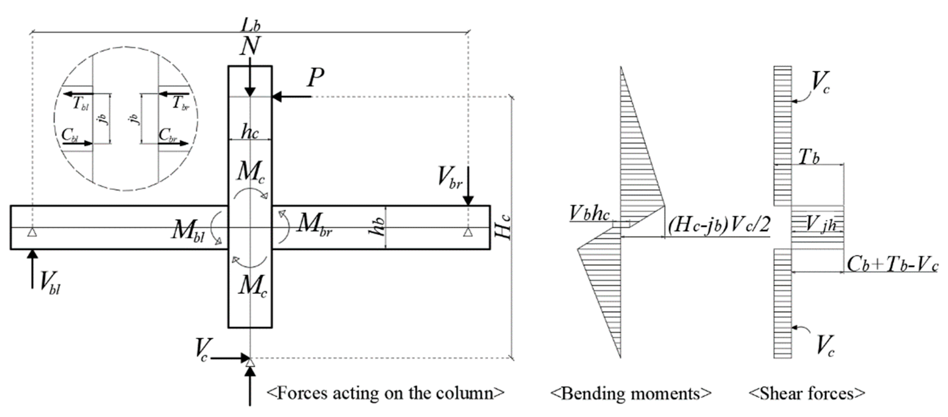
Appendix A.2. Shear Strength of Beam–Column Joint

In ASCE 41, the joint shear strength V j n is specified as
V j n = 0.083 γ f c A j
where γ is a factor reflecting the confinement provided by the transverse beam and joint shear reinforcement, and A j represents the effective joint area. Interior joints with s 0.5 h c are classified as conforming joints, and γ = 15 is used. Interior joints with s > 0.5 h c are classified as nonconforming joints, and γ = 10 is used. Here, s represents the spacing of the joint transverse reinforcement, and h c represents the column depth measured in the direction of the joint shear considered.
In Figure A1, the sum of the vertical forces at the beam supports is ( V b l + V b r ) = 2 P · ( H c / L b ) , and the sum of the beam moments at the joint faces is ( M b l + M b r ) = P · ( H c / L b ) · ( L b h c ) . Hence, the horizontal shear force at the joint V j is expressed as
V j = T b l + T b r P = M b l + M b r j b P = P ( H c L b ) ( L b h c j b ) P
where j b represents the moment lever arm of the beam section ( 0.87 d e f f ; Joh et al. [16] and Kamimura et al. [18]), and d e f f represents the effective depth of the beam. When joint shear failure occurs [i.e., V j = V j n in Equation (A3)], the corresponding lateral force P n j is defined as follows:
P n j = V j n ( H c L b ) ( H c h c j b L b ) 1

Appendix A.3. Bond Strength of Beam Reinforcement

In ACI 318, the minimum embedment length of all the straight beam and column bars passing through the joint is defined as
h c 20 d b
where d b represents the diameter of the largest beam longitudinal reinforcing bar. When the embedment length of the beam reinforcement is shorter than the required value, bond failure is expected in the joint.

Appendix A.4. Strength Predictions for Test Specimens

Table A1 presents the nominal strengths P n b , P n c , and P n j under beam yielding, column yielding, and joint shear failure, respectively, which were calculated via Equations (A1)–(A6) using the actual material strengths. Specimens S16-N, S13-N, and U13-N were classified as nonconforming joints according to the ASCE 41 requirement, as the shear reinforcement is not provided in the joint. For these joints, P n j is denoted as P n j N C . For S16-32, S16-34, S13-32, S13-34, and U13-34, where the hoop spacing satisfies the requirement,   P n j is denoted as P n j C . It is noted that ASCE 41 does not specify the shape and details of joint hoops apart from the spacing.
As shown in Table A1, for S16-N, S13-N, and U13-N, P n j N C was smaller than P n b and P n c , indicating that joint shear failure was expected. However, for S16–32, S16–34, S13–32, and S13–34, P n j C was the lowest among strengths under the lateral loading. Among the specimens, U13–34 had the closest P n j C to the force P n b at the beam yielding point. Therefore, among the eight specimens, seven exhibited joint shear failure before the yielding of the beam, and only one failed after beam yielding. Table A1 presents the provided and required anchorage lengths of the beam flexural reinforcements ( l a l and l d h , respectively). The l a l / l d h ratios of 0.78 and 0.96 indicate that the anchorage length was satisfied for the Group 2 and 3 specimens but not for Group 1. Therefore, the test specimens were designed to induce joint shear failure, with consideration of the effect of the insufficient anchorage length.
Table A1. Prediction of the Nominal Strengths and Failure Modes *.
SpecimenColumn YieldingBeam YieldingJoint Shear Failure Predicted   Strength ,   P n   ( kN ) Failure ModeAnchorage Length
M n c ,   ( kN · m ) P n c ,   ( kN ) M n , b l ,   ( kN · m ) M n , b r ,   ( kN · m ) P n b ,   ( kN ) ConformingNonconforming
V j n C ,   ( kN ) P j n C ,   ( kN ) V j n N C ,   ( kN ) P j n N C ,   ( kN ) l a l   ( mm ) l a l l d h
S16-N78.012551.651.676.4--247.9339.939.9J2500.78
S16-3277.712451.551.576.336759.1--59.1J2500.78
S16-3478.212551.651.676.437560.2--60.2J2500.78
S13-N62.810057.457.485.0--25440.940.9J2500.96
S13-3263.010157.857.885.638962.7--62.7J2500.96
S13-3463.110157.857.885.639162.8--62.8J2500.96
U13-N79.912856.942.173.3--26442.442.4J2500.96
U13-3479.912856.942.173.339663.6--63.6BJ2500.96
* Note: J = joint shear failure; BJ = beam joint failure;   l a l and l d h = provided and required anchorage length, respectively; P n c and P n b = connection strengths by column and beam yielding; and P n j = connection strength by joint failure (ASCE 41).

Appendix B. Constitutive Model for Nonlinear Fe Analysis of Test Specimens

Appendix B.1.Constitutive Law for Concrete

In the analysis, a total strain-based rotating crack model was used for nonlinear concrete. An isotropic linear–elastic material model based on Young’s modulus and Poisson’s ratio was adopted for linear concrete. The Poisson’s ratio was assumed to be 0.15 regardless of the concrete strength. Young’s modulus obtained from the material test was used.

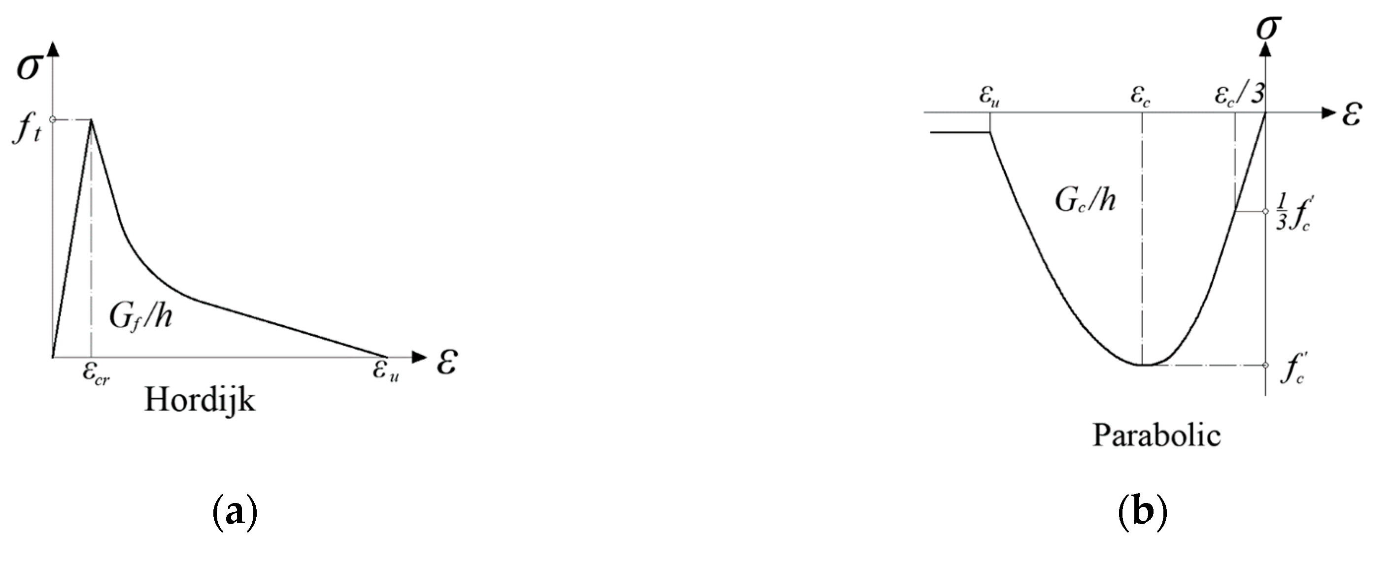
Appendix B.1.1. Tensile Behavior

DIANA 10.3 [34] predefines tensile stress–strain curves for the total strain crack model. In the present study, the nonlinear tension-softening model proposed by Hordijk [34] was adopted for nonlinear FE analysis (NFEA), as the tension-softening model results in more localized cracks and consequently avoids large areas of diffuse cracking. The stress–strain relationship for concrete under tension is shown in Figure A2a. Here, the parameters are the tensile strength f t , fracture energy G f , and crack bandwidth, h .
Figure A2. Model for concrete: (a) predefined tensile stress–strain curve; (b) predefined compressive stress–strain curve.
Buildings 10 00176 g0a2
The uniaxial tensile strength of concrete f t was determined using the compressive strength f c according to the CEB-FIB Model code (1990) [32]:
f t = 0.3 ( f c ) 2 / 3 .
The tensile fracture energy of concrete, i.e., G f ( N / mm 2 ), was determined using the formula of the CEB-FIB Model code:
G f = ( 73 f c 0.18 ) / 1000
where f c represents the compressive strength of the concrete.
The crack bandwidth h is an essential parameter in constitutive models that describes the softening stress–strain relationship. Additionally, it is crucial to reduce the mesh-size dependence. In this study, an automatic procedure for determining the crack bandwidth provided in DIANA 10.3 was used.

Appendix B.1.2. Compressive Behavior

In DIANA 10.3, the compressive behavior of the total strain crack model can be described using predefined curves. A parabolic stress–strain diagram with a softening branch was used in this study (Figure A2b). The softening branch was determined according to the compressive fracture energy, G c , to reduce the mesh-size dependence during compressive-strain localization. The compressive fracture energy of concrete, i.e., G c ( N / mm 2 ), was determined using the formula proposed by Nakamura and Higai [35]:
G c = 250 G f .
The lateral influence on the concrete mainly comprised two aspects. The first was the decrease in the compressive strength of the concrete, which occurred because the tensile strain perpendicular to the principal compressive stress caused cracks and damage in the concrete. The reduction is explained by the model developed by Vecchio and Collins [36] in DIANA 10.3. The other aspect is the lateral confinement. It has long been recognized that the strength, as well as the deformability of concrete, continuously increases when the amount of confinement is increased. Equations have been proposed based on numerous experimental studies to predict the improvement of the loading capacity. In DIANA 10.3, the effects of the lateral confinement are considered by modifying the compressive stress–strain curves, for which the parameters are determined by a failure function defining the compressive stress as a function of the confining stresses in the lateral directions, as explained by the model of Selby et al. [37].

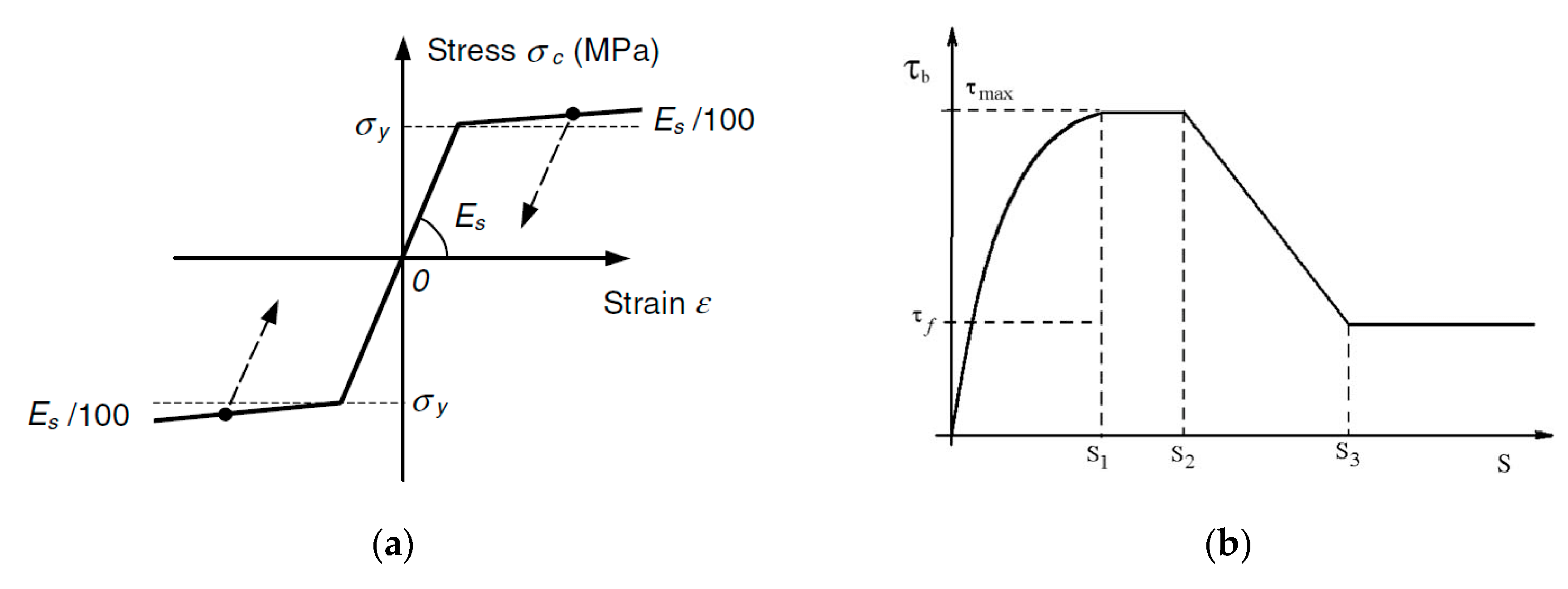
Appendix B.2. Constitutive Law for Reinforcement

The von Mises criterion with isotropic strain hardening and the associated flow rule was used to describe the constitutive behavior of the reinforcement. The bars were modeled with the DIANA options of separate truss elements. Figure A3a shows the stress–strain relationship for the reinforcing steel, which was modeled with an elastoplastic curve. During the test, bond deterioration was observed along the beam longitudinal bars and main column bars (particularly within the joint region), and slippage of the steel bars was expected to occur. The bond–slip models with the DIANA options accounted for the reinforcement and surrounding concrete.
Figure A3. Model for the reinforcement: (a) stress–strain curve for the steel reinforcement; (b) bond–slip law based on CEB-Figure 1990.
Buildings 10 00176 g0a3

Bond–Slip Law

The bond law used in the analysis is based on the CEB-FIP model code 1990, as shown in Figure A3b. Equations of the bond stress for different parts of the curve are presented below:
τ = τ max ( s s 1 ) α   for   0 s s 1
τ = τ max   for   s 1 s s 2
τ = τ max ( τ max τ f ) s s 1 s 3 s 2   for   s 2 s s 3
τ = τ f   for   s 3 s .
The bond-law model parameters were s 1 = 1.0 mm, s 2 = 3.0 mm, s 3 = 5.0 mm, α = 0.4, τ max = 2 f c , and τ f = 0.4 τ max .

Appendix B.3. Geometry Modeling

Eight-node two-dimensional quadratic solid elements (CQ16M) were used for the concrete modeling, and the embedded reinforcing bars were modeled using truss elements. As an example, the FE discretization of the specimens is presented in Figure A4.
Figure A4. Two-dimensional FE discretization of the specimen.
Buildings 10 00176 g0a4

Appendix C. Analysis Variables of Parametric Study

Table A2 lists the main analysis parameters of 39 FE beam–column joint models that were used to develop three equations to predict the joint shear deformation index (SDI) of interior joints for various combinations of joint design parameters.
Table A2. Specimen Properties and Analysis Variables.
SpecimensGeometric PropertiesTop Rebar of BeamBottom Rebar of BeamJoint Hoop RatioJoint Aspect RatioArea RatioStrength RatioFailure Mode
(a)(b)(c) (d)
LHhcbchbbbdbAsfydbAsfyρj, (%) h b / h c A c / A b   M c M b FE Prediction
Group 1M160003000600600500400221548431191146431-0.831.82.5B
M20.30.831.82.5B
M30.60.831.82.5B
M4252026-0.831.82.2B
M50.30.831.82.2B
M60.60.831.82.2B
M7600400221548-1.01.52.0BJ
M80.241.01.52.0B
M90.481.01.52.0B
M10252026-1.01.51.7BJ
M110.241.01.51.7B
M120.481.01.51.7B
M13700400221548-1.171.291.7BJ
M140.21.171.291.7B
M150.41.171.291.7B
M16252026-1.171.291.5BJ
M170.21.171.291.5B
M180.41.171.291.5B
Group 2M1960003000500500500400221548-1.01.251.7B
M200.361.01.251.7B
M210.721.01.251.7B
M22252026-1.01.251.5BJ
M230.361.01.251.5B
M240.721.01.251.5B
M25600400221548-1.21.041.4BJ
M260.291.21.041.4BJ
M270.571.21.041.4B
M28252026-1.21.041.2J
M290.291.21.041.2BJ
M300.571.21.041.2B
M31700400221548-1.40.891.2J
M320.241.40.891.2BJ
M330.481.40.891.2B
M34252026-1.40.891.0J
M350.241.40.891.0BJ
M360.481.40.891.0B
M37550550600400252026-1.11.261.46BJ
M380.261.11.261.46B
M390.521.11.261.46B
(a) L = beam length (mm); H = column height (mm); hc = column depth (mm); bc = column width (mm); hb = beam depth (mm); bb = beam width (mm); (b) db = rebar diameter (mm); As = area of rebar (mm2); and fy = yield strength of rebar (MPa); (c) yield strength of joint hoop is assumed to be 345 MPa; (d) B = beam failure; BJ = beam joint failure (joint failure after beam yield); and J = joint failure (joint failure before beam yield.

Appendix D. Summary of Beam–Column Connection Tests

Table A3 lists the main analysis parameters of 50 existing beam–column joints that were used to verify the proposed equations.
Table A3. Analysis Parameters of Existing Test Specimens.
Research TeamSpecimensJoint Hoop RatioJoint Aspect RatioArea RatioStrength RatioMechanical Reinforcement RatioSDI at 2.5%SDI at 3.5%Failure Mode
ρj, (%) h b h c A c A b M c M b A s , t o p f y b b d f c R s p s R s R s p s R s Test Result
Fuji and Morita (1991) [17]A10.521.141.211.240.500.620.69J
A20.521.141.212.020.190.410.62J
A30.521.141.211.240.500.650.72J
A40.691.141.211.240.500.690.72J
Joh et al. (1991 [16])HL1.271.171.292.410.090.030.04B
MH0.551.171.292.410.090.030.05B
B91.11.171.292.410.100.050.07B
B101.11.171.292.410.100.060.09B
B111.11.171.292.410.100.070.10B
Noguchi and Kashiwazaki (1992) [38]J10.661.001.501.530.240.400.48BJ
J30.661.001.501.480.170.370.41J
J40.661.001.501.530.240.370.48BJ
J50.661.001.501.370.260.310.40J
J60.661.001.501.470.270.300.33J
Oka and Shiohara (1992) [39]J10.461.001.251.720.150.400.60BJ
J70.461.001.252.120.130.100.13B
J100.461.001.251.350.340.440.58J
Kimamura et al. (2000) [18]No.10.151.001.391.70.240.470.53J
No.20.311.001.391.70.240.510.44J
No.30.621.001.391.70.240.420.44J
No.40.311.001.392.560.160.110.11B
No.50.621.001.392.560.160.080.08B
Li and Leong (2014) [40]NS10.711.111.082.110.07N/A 0.09B
AS10.711.111.083.590.07N/A 0.03B
NS20.481.111.081.860.03N/A 0.10B
AS20.481.111.083.90.03N/A 0.03B
NS30.711.111.082.350.07N/A 0.09B
AS30.711.111.083.830.07N/A 0.03B
NS40.571.111.082.820.03N/A 0.11B
AS40.571.111.085.150.03N/A 0.03B
Hwang et al. (2014) [41]C1-4001.340.911.571.670.310.180.20BJ
C2-6001.340.911.571.680.270.140.18BJ
C3-6001.340.911.411.220.270.150.19BJ
C4-6001.340.911.571.880.270.160.19BJ
Melo et al. (2014) [42]IPA-101.670.600.940.060.600.82J
IPA-201.670.600.990.040.400.75J
IPB01.670.600.960.060.500.62J
IPE01.670.601.230.060.360.75J
ID01.670.600.880.070.520.77J
Alaee and Li (2017) [43]IN800.711.111.081.710.050.140.11B
IH800.571.111.082.180.060.260.20BJ
IH80A0.571.111.083.750.060.050.05B
IN1000.711.111.081.720.040.260.20BJ
IH1000.711.111.082.190.050.310.29BJ
IH600.571.111.082.290.060.310.25BJ
IH60A0.571.111.083.230.060.090.07B
Yang and Zhao (2018) [44]CL11.171.250.911.230.130.270.61BJ
CL21.541.251.071.240.190.370.73BJ
CL31.600.891.581.370.230.410.73BJ
CL41.541.251.071.140.160.340.61BJ

References

  1. Kitayama, K.; Otani, S.; Aoyama, H. Development of Design Criteria for RC Interior Beam-Column Joints. ACI Struct. J. 1991, SP-123, 97–123. [Google Scholar]
  2. Bonacci, J.; Pantazopoulou, S. Parametric investigation of joint mechanics. ACI Struct. J. 1993, 90, 61–71. [Google Scholar] [CrossRef]
  3. Shiohara, H.; Kobayashi, F.; Sato, Y.; Kusuhara, F. Earthquake response of multi-story reinforced concrete plane frame structures and seismic design of beam-column joints. J. Struct. Constr. Eng. 2017, 82, 1437–1447. [Google Scholar] [CrossRef]
  4. Nagae, T.; Ghannoum, W.M.; Kwon, J.; Tahara, K.; Fukuyama, K.; Matsumori, T.; Shiohara, H.; Kabeyasawa, T.; Kono, S.; Nishiyama, M.; et al. Design implications of large-scale shake-table test on four-story reinforced concrete building. ACI Struct. J. 2015, 112, 135–146. [Google Scholar] [CrossRef]
  5. Hakuto, S.; Park, R.; Tanaka, H. Effect of deterioration of bond of beam bars passing through interior beam-column joints on flexural strength and ductility. ACI Struct. J. 1999, 96, 858–864. [Google Scholar] [CrossRef]
  6. Paulay, T.; Park, R.; Priestley, M.J.N. Reinforced Concrete Beam-Column Joints Under Seismic Actions. ACI Struct. J. 1978, 75, 585–593. [Google Scholar]
  7. Ichinose, T. Interaction Between Bond at Beam Bars and Shear Reinforcement in R/C Interior Joints. ACI Struct. J. 1991, 123, 379–400. [Google Scholar]
  8. British Standards Institution. Eurocode 8: Design of Structures for Earthquake Resistance-Part 1: General Rules, Seismic Actions and Rules for Buildings; British Standards Institution: London, UK, 2005. [Google Scholar]
  9. Standards New Zealand. Concrete Structures Standard—The Design of Concrete Structures; NZ S3101-12006; Standards New Zealand: Wellington, New Zealand, 2017; Volume 1, ISBN 1-86975-043-8. [Google Scholar]
  10. ACI Committee 318. Building Code Requirements for Structural Concrete (ACI318-14) and Commentary (318R-14); American Concrete Institute: Farmington Hills, MI, USA, 2014; p. 443. [Google Scholar]
  11. Otani, S. The architectural institute of Japan proposal of ultimate strength design requirements for RC buildings with emphasis on beam-column joints. ACI Struct. J. 1991, SP-123, 125–144. [Google Scholar]
  12. Shiohara, H. New model for shear failure of RC interior beam-column connections. J. Struct. Eng. 2001, 127, 152–160. [Google Scholar] [CrossRef]
  13. Shiohara, H. Reinforced concrete beam-column joints: An overlooked failure mechanism. ACI Struct. J. 2012, 109, 65–74. [Google Scholar]
  14. Shiohara, H.; Kusuhara, F. Joint Shear? or Column-to-Beam Strength Ratio? Which is a key parameter for seismic design of RC Beam-column joints—Test Series on Interior Joints. In Proceedings of the 15th World Conference on Earthquake Engineering, Lisbon, Portugal, 24–28 September 2012; pp. 1–9. [Google Scholar]
  15. American Society of Civil Engineers. Seismic Evaluation and Retrofit of Existing Structures ASCE/SEI 41-13; American Society of Civil Engineers: Reston, VA, USA, 2014; p. 554. [Google Scholar]
  16. Joh, O.; Goto, Y.; Shibata, T. Influence of Transverse Joint and Beam Reinforcement and Relocation of Plastic Hinge Region on Beam Column Joint Stiffness Deterioration. ACI Struct. J. 1991, 123, 187–224. [Google Scholar] [CrossRef]
  17. Fuji, S.; Morita, S. Comparison between Interior and Exterior R/C Beam-Column Joint Behavior, Design of Beam-Column Joints for Seismic Resistance. ACI Struct. J. 1991, 132, 145–166. [Google Scholar]
  18. Kamimura, T.; Takeda, S.; Tochio, M. Influence of joint reinforcement on strength and deformation of interior beam-column subassemblages. In Proceedings of the 12th World Conference on Earthquake Engineering, Auckland, New Zealand, 30 January–4 February 2000; p. 2267. [Google Scholar]
  19. Kim, J.; LaFave, J.M. Key influence parameters for the joint shear behaviour of reinforced concrete (RC) beam-column connections. Eng. Struct. 2008, 29, 2523–2539. [Google Scholar] [CrossRef]
  20. Hwang, S.J.; Lee, H.J.; Liao, T.F.; Wang, K.C.; Tsai, H.H. Role of hoops on shear strength of reinforced concrete beam-column joints. ACI Struct. J. 2005, 102, 445–453. [Google Scholar] [CrossRef]
  21. Hwang, S.J.; Lee, H.J. Analytical model for predicting shear strengths of interior reinforced concrete beam-column joints for seismic resistance. ACI Struct. J. 2000, 97, 35–44. [Google Scholar] [CrossRef]
  22. Hwang, S.J.; Tsai, R.J.; Lam, W.K.; Moehle, J.P. Simplification of softened strut-and-tie model for strength prediction of discontinuity regions. ACI Struct. J. 2017, 114, 1239–1248. [Google Scholar] [CrossRef]
  23. Hong, S.G.; Lee, S.G.; Kang, T.H.K. Deformation-based strut-and-tie model for interior joints of frames subject to load reversal. ACI Struct. J. 2011, 108, 423–433. [Google Scholar] [CrossRef]
  24. Hwang, H.J.; Eom, T.S.; Park, H.G. Shear strength degradation model for performance-based design of interior beam-column joints. ACI Struct. J. 2017, 114, 1143–1154. [Google Scholar] [CrossRef]
  25. Lee, J.-Y.; Park, J.; Kim, C. Deformations of reinforced-concrete beam-column joint assemblies. Mag. Concr. Res. 2020, 72, 649–669. [Google Scholar] [CrossRef]
  26. Tajiri, S.; Fukuyama, H.; Suwada, H.; Kusuhara, F.; Shiohara, H. Energy Dissipation of RC Interior Beam-column Connection Confined by Lateral Reinforcements, Axial Force, and Column Longitudinal Reinforcements. In Proceedings of the 15th World Conference on Earthquake Engineering, Lisbon, Portugal, 24–28 September 2012. [Google Scholar]
  27. Park, R. Ductility evaluation from laboratory and analytical testing. In Proceedings of the 9th World Conference on Earthquake Engineering, Tokyo, Japan, 2–9 August 1988; pp. 605–616. [Google Scholar]
  28. ACI Committee 374. Commentary on Acceptance Criteria for Moment Frames Based on Structural Testing; (ACI 374.1-05); American Concrete Institute: Farmington Hills, MI, USA, 2002. [Google Scholar]
  29. Kusuhara, F.; Shiohara, H. New instrumentation for damage and stress in reinforced concrete beam-column joint. In Proceedings of the 8th U.S. National Conference on Earthquake Engineering, San Francisco, CA, USA, 18–22 April 2006; Volume 7, pp. 4006–4015. [Google Scholar]
  30. Joint ACI-ASCE Committee 352. Recommendations for Design of Beam-Column Connections in Monolithic Reinforced Concrete Structures; (ACI 352R-02); American Concrete Institute: Farmington Hills, MI, USA, 2002. [Google Scholar]
  31. DIANA Version 10.3; Computer software; TNO Building and Construction Research: Delft, The Netherlands, 2019.
  32. Design of Concrete Structures: CEB-FIP Model-Code 1990; Thomas Telford Service Ltd.: London, UK, 1990.
  33. Deaton, J.B. Nonlinear Finite Element Analysis of Reinforced Concrete Exterior Beam-Column Joints with Nonseismic Detailing. Ph.D. Thesis, Georgia Institute of Technology, Atlanta, GA, USA, 2013; pp. 1–315. [Google Scholar]
  34. Hordijk, D.A. Local Approach to Fatigue of Concrete. Ph.D. Thesis, Delft University of Technology, Delft, The Netherlands, 1991. [Google Scholar]
  35. Nakamura, H.; Higai, T. Compressive fracture energy and fracture zone length of Concrete, Modelling of inelastic behavior of RC structures under seismic loads edited by Shing, P., Tanabe, T. ASCE 1999, 10, 471–487. [Google Scholar]
  36. Vecchio, F.J.; Collins, M.P. Compression response of cracked reinforced concrete. J. Struct. Eng. 1993, 119, 3590–3610. [Google Scholar] [CrossRef]
  37. Selby, R.G.; Vecchio, F.J.; Collins, M.P. Analysis of reinforced concrete members subject to shear and axial compression. ACI Struct. J. 1996, 93, 306–315. [Google Scholar]
  38. Noguchi, H.; Kashiwazaki, T. Experimental studies on shear performances of RC interior column-beam joints with high-strength materials. In Proceedings of the 10th World Conference on Earthquake Engineering, Madrid, Spain, 19–24 July 1992. [Google Scholar]
  39. Oka, J.; Shiohara, H. Tests of high-strength concrete interior beam-column-joint subassemblages. In Proceedings of the 10th World Conference on Earthquake Engineering, Madrid, Spain, 19–24 July 1992. [Google Scholar]
  40. Li, B.; Leong, C.L. Experimental and numerical investigations of the seismic behavior of high-strength concrete beam-column joints with column axial load. J. Struct. Eng. 2015, 141, 04014220. [Google Scholar] [CrossRef]
  41. Hwang, H.J.; Park, H.G.; Choi WSChung, L.; Kim, J.K. Cyclic loading test for beam-column connections with 600 MPa (87 ksi) beam flexural bars. ACI Struct. J. 2014, 111, 913–924. [Google Scholar] [CrossRef]
  42. Melo, J.; Varum, H.; Rossetto, T. Cyclic behavior of interior beam-column joints reinforced with plain bars. Earthq. Eng. Struct. Dyn. 2015, 44, 1351–1371. [Google Scholar] [CrossRef]
  43. Alaee, P.; Li, B. High-strength concrete interior beam-column joints with high-yield-strength steel reinforcements. J. Struct. Eng. 2017, 143, 04017038. [Google Scholar] [CrossRef]
  44. Yang, H.; Zhao, W.; Zhu, Z.; Fu, J. Seismic behavior comparison of reinforced concrete interior beam-column joints based on different loading methods. Eng. Struct. 2018, 116, 31–45. [Google Scholar] [CrossRef]
Figure 1. Dimensions and reinforcement details of the specimens. (a) Group 1 and Group 3 specimens, (b) Group 2 specimens.
Buildings 10 00176 g001aBuildings 10 00176 g001b
Figure 2. Details of joint shear reinforcements (unit in mm).
Buildings 10 00176 g002
Figure 3. Schematic of the test setup.
Buildings 10 00176 g003
Figure 4. Photograph of the test setup.
Buildings 10 00176 g004
Figure 5. Displacement-controlled loading history.
Buildings 10 00176 g005
Figure 6. (a) Measurement system for the joint deformation and fixed end rotation; (b) strain-gauge locations (unit in mm).
Buildings 10 00176 g006
Figure 7. Measurement mechanism of the system: (a) For chord rotations and fixed end rotations; (b) For deformation of joint.
Buildings 10 00176 g007
Figure 8. Experimental and analytical lateral load–drift ratio relationships.
Buildings 10 00176 g008aBuildings 10 00176 g008b
Figure 9. Failure modes at the end of the test: (a) S16-N; (b) S13-N; (c) U13-N; (d) S16-32; (e) S13-32; (f) S16-34; (g) S13-34; (h) U13-34.
Buildings 10 00176 g009aBuildings 10 00176 g009b
Figure 10. Strain distributions of the beam flexural reinforcement: (a) S13-N; (b) S13-32; and (c) S13-34.
Buildings 10 00176 g010aBuildings 10 00176 g010b
Figure 11. Relationship between the normalized joint shear stress and the lateral drift angle.
Buildings 10 00176 g011
Figure 12. Decomposition of the lateral drift of the interior beam–column joint: (a) percentage of deformation for Groups 1, 2, and 3 at a lateral drift of 3.5%; (b) deformation components.
Buildings 10 00176 g012
Figure 13. Strain development of the joint shear reinforcement: (a) S13-34 and (b) U13-34.
Buildings 10 00176 g013
Figure 14. Envelope curves for the joint shear stress versus joint shear strain.
Buildings 10 00176 g014
Figure 15. Diagonal elements of the joint panel in the finite element (FE) models.
Buildings 10 00176 g015
Figure 16. Maximum shear stress at the interior joints for different combinations of design variables: (a) no joint reinforcement ratio; (b) low joint reinforcement ratio; (c) moderate joint reinforcement ratio; (d) total design variables.
Buildings 10 00176 g016aBuildings 10 00176 g016b
Figure 17. Shear deformation index (SDI) of interior connections for different combinations of design variables: (a) low ductility demand (<2); (b) moderate ductility demand (2–4); and (c) high ductility demand (>4).
Buildings 10 00176 g017aBuildings 10 00176 g017b
Figure 18. SD index corresponding to J-Failure.
Buildings 10 00176 g018
Figure 19. SD index corresponding to BJ-Failure.
Buildings 10 00176 g019
Figure 20. SD index corresponding to B-Failure.
Buildings 10 00176 g020
Figure 21. Experimental shear deformation index (SDI) versus the SDI predicted by proposed equations: (a) J-mode predicted by Equation (3); (b) BJ-mode predicted by Equation (4); and (c) B-mode predicted by Equation (5).
Buildings 10 00176 g021aBuildings 10 00176 g021b
Table 1. Specimen Properties and Test Variables.
SpecimensS16-NS16-32S16-34S13-NS13-32S13-34U13-NU13-34
Concrete Strength, f c (MPa)28.227.528.629.730.931.132.131.9
Axial Load Ratio, ( N u / f c A g )0.070.080.070.070.070.070.070.07
BeamWidth × Depth in mm200 × 250200 × 250200 × 250
Top Rebar, %1.351.441.44
Bottom Rebar, %1.351.440.88
ColumnWidth × Depth in mm250 × 250250 × 250250 × 250
Reinforcing Bar Ratio (%)2.431.622.43
JointHoop Ratio ρ j (%)-0.360.72-0.360.72-0.72
Flexural Strength Ratio1.51.51.51.11.11.11.61.6
Joint Demand Ratio ( V j n / V j )0.820.760.91
Anchorage Length Ratio ( h c / d b ) 15.619.219.2
Table 2. Material Test Results for the Reinforcing Bars.
DiameterGrade Yield   Strength ,   f y ,   ( MPa ) Yield   Strain ,   ε y   ( µ ) Ultimate   Strength ,   f u ,   ( MPa ) Elastic   Modulus ,   E s   ( GPa )
D6SD3453631998542182
D13SD3904982602669192
D164402449618180

