
Mechanical Fracture of Aluminium Alloy (AA 2024-T4), Used in the Manufacture of a Bioproducts Plant


Abstract
:1. Introduction
2. Materials and Methods
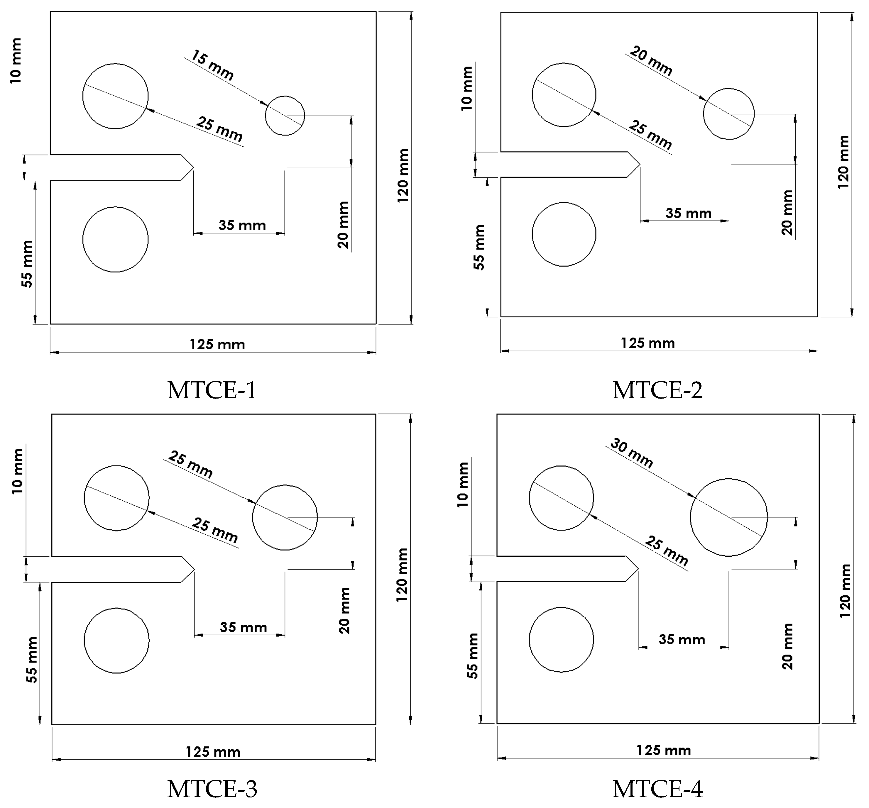
2.1. Material and Specimens
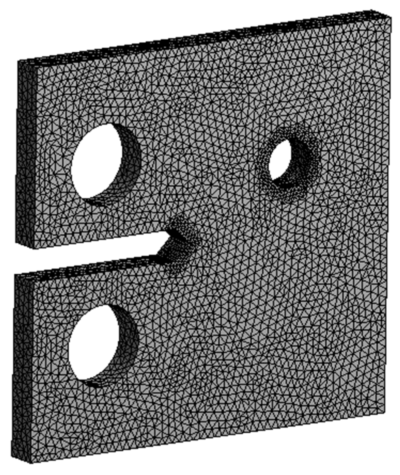
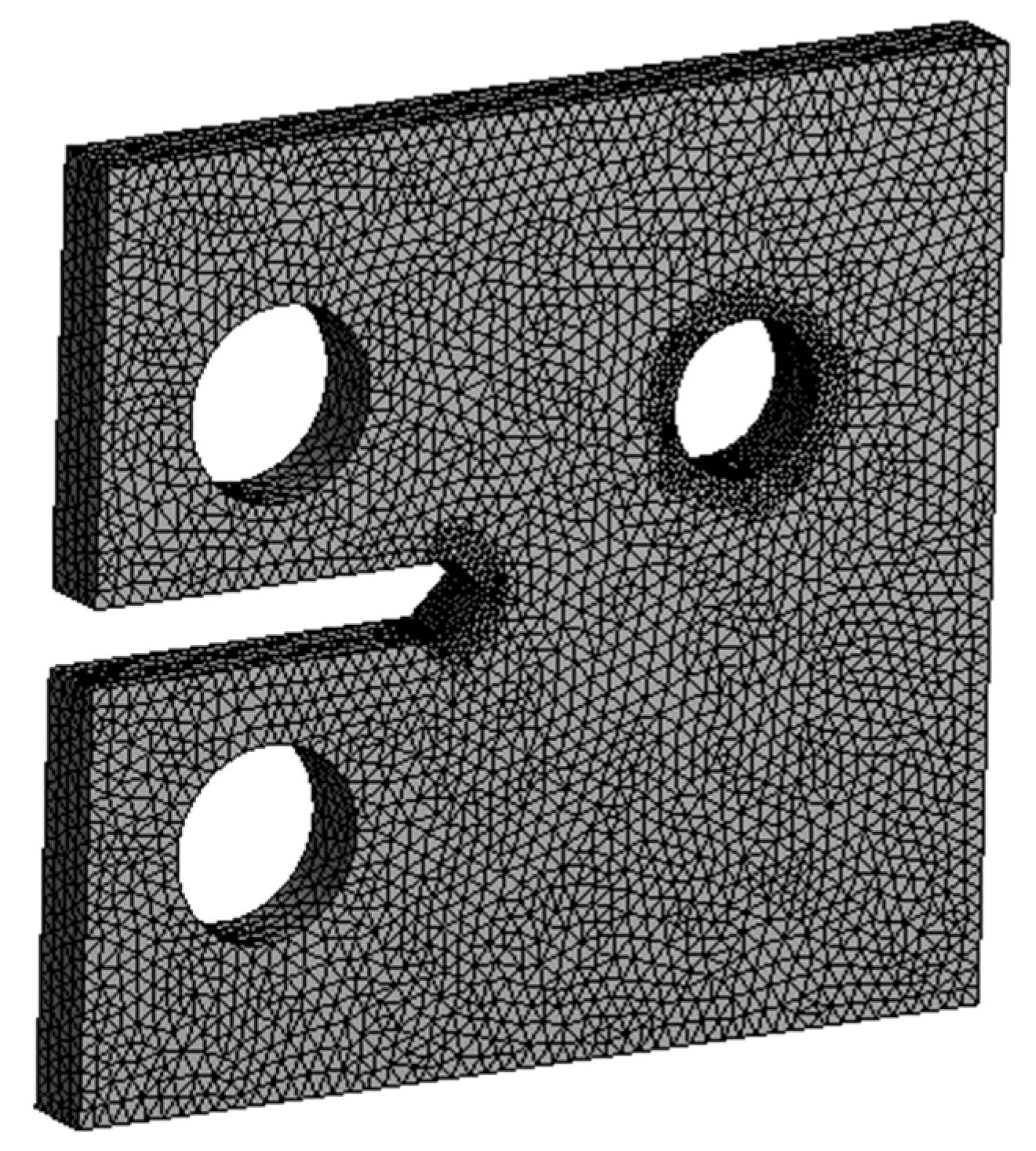
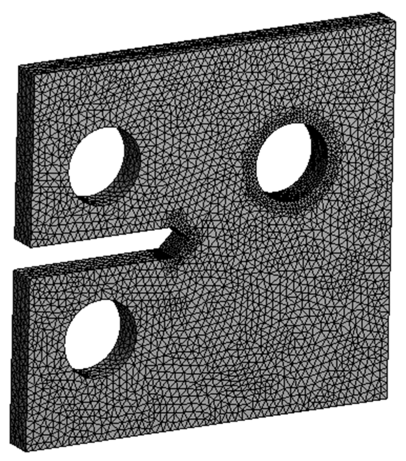
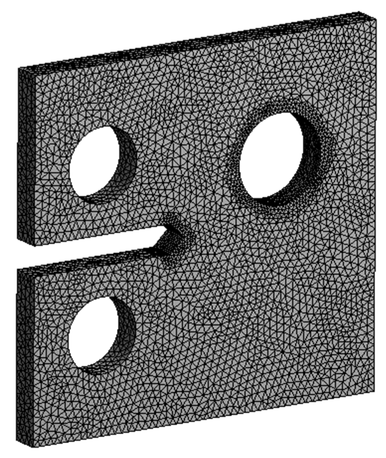
2.2. Computational Model Using SMART Method
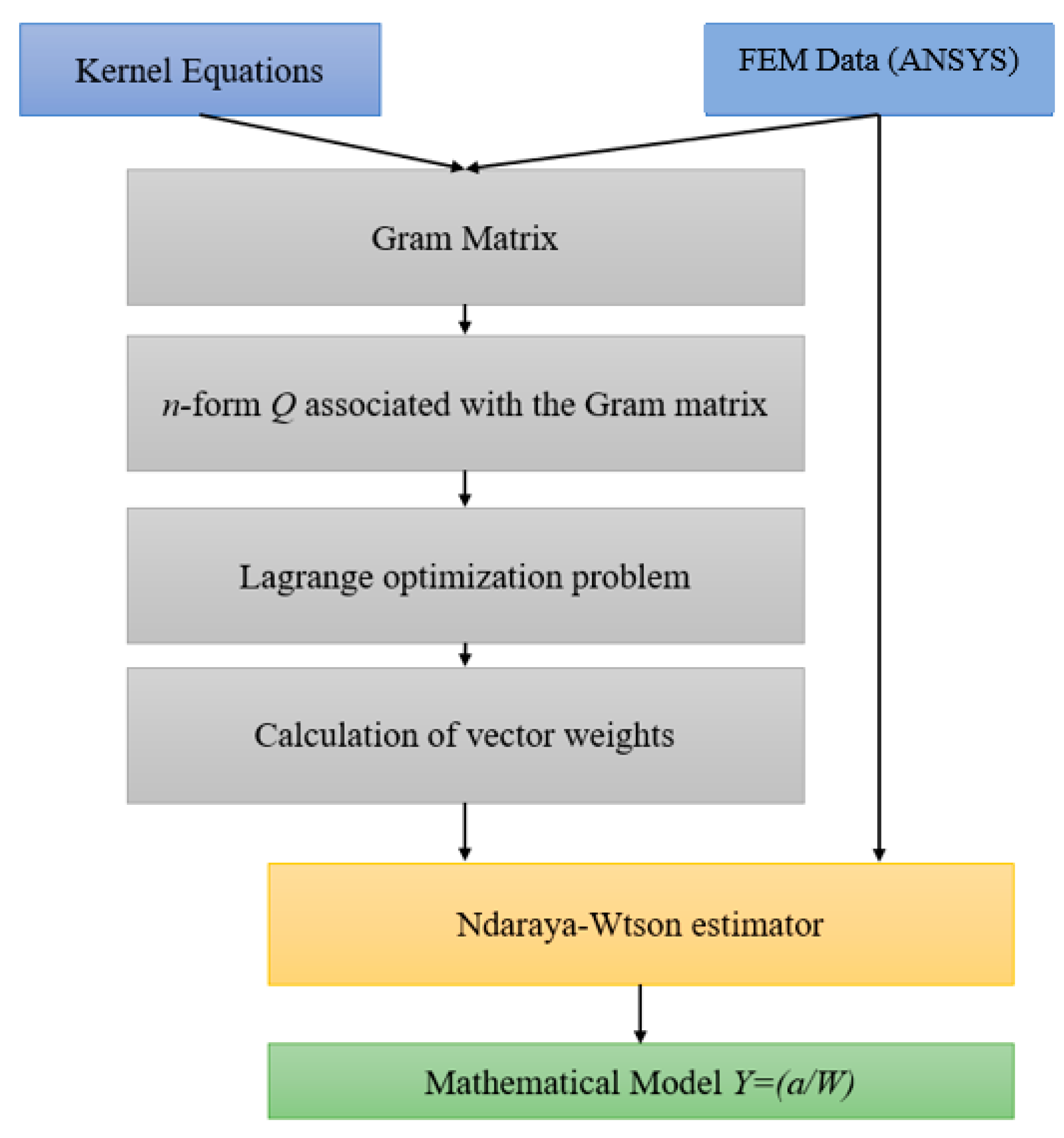
2.3. Data Processing Using Support Vector Regression (SVR) and Nadaraya-Watson Estimator (NWE)
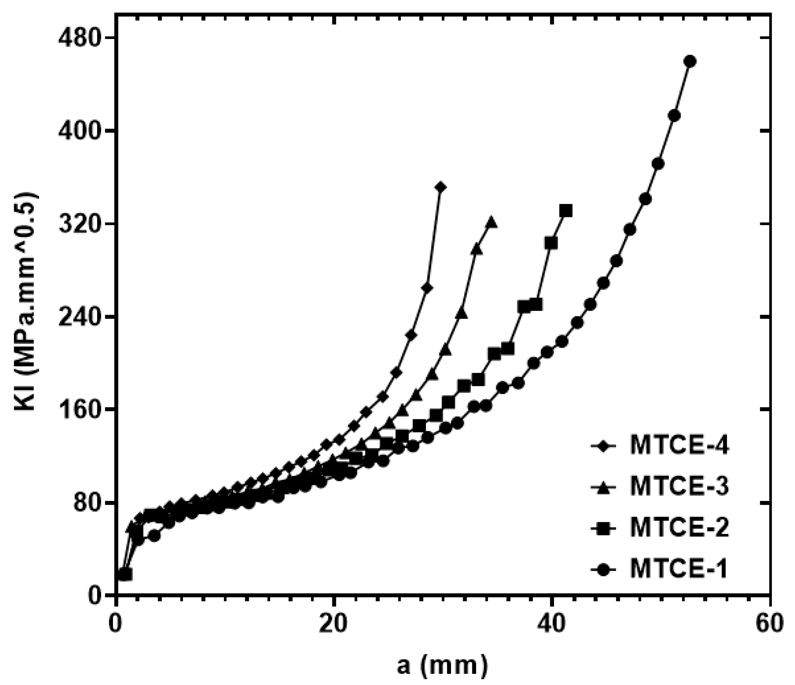
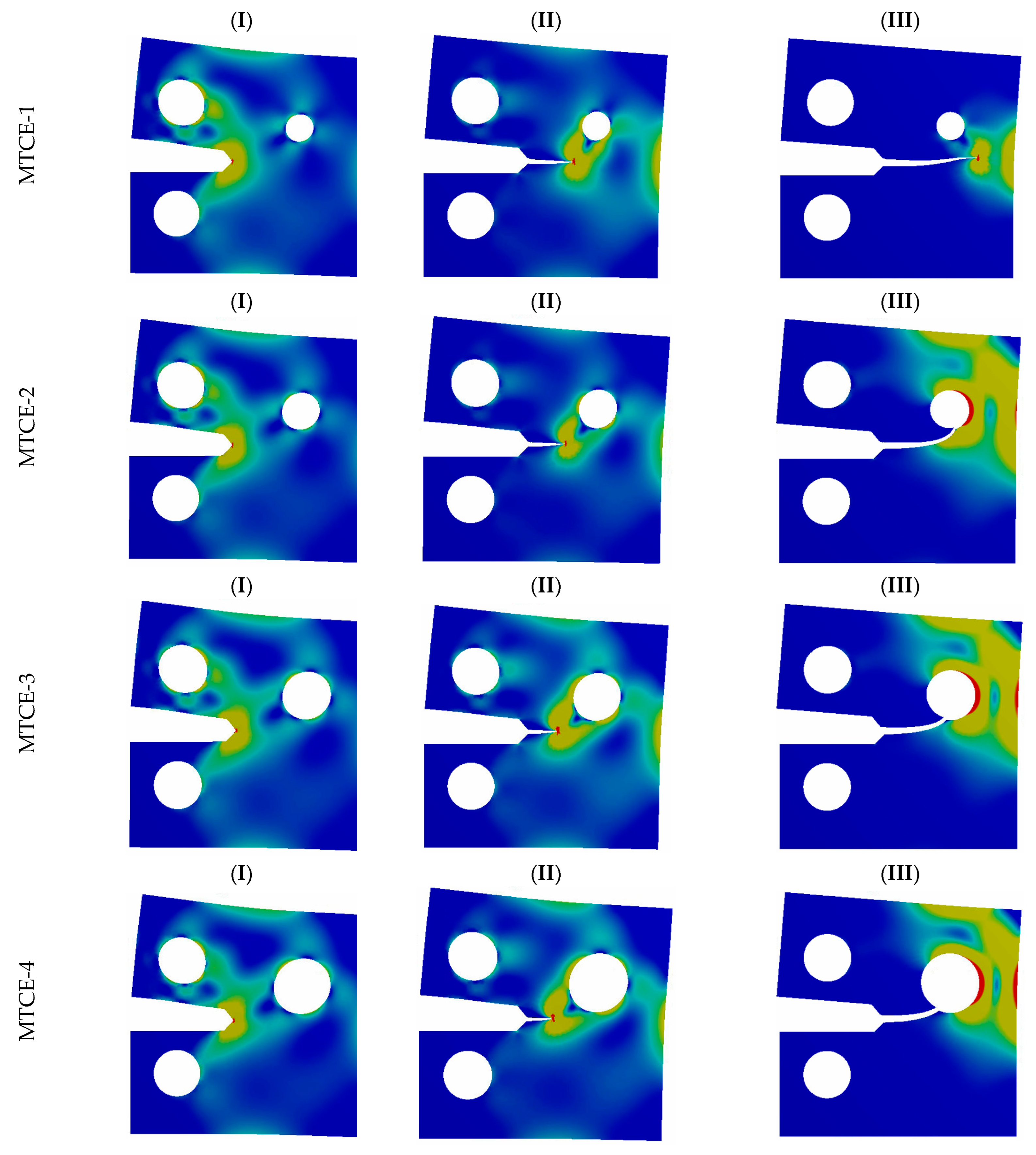
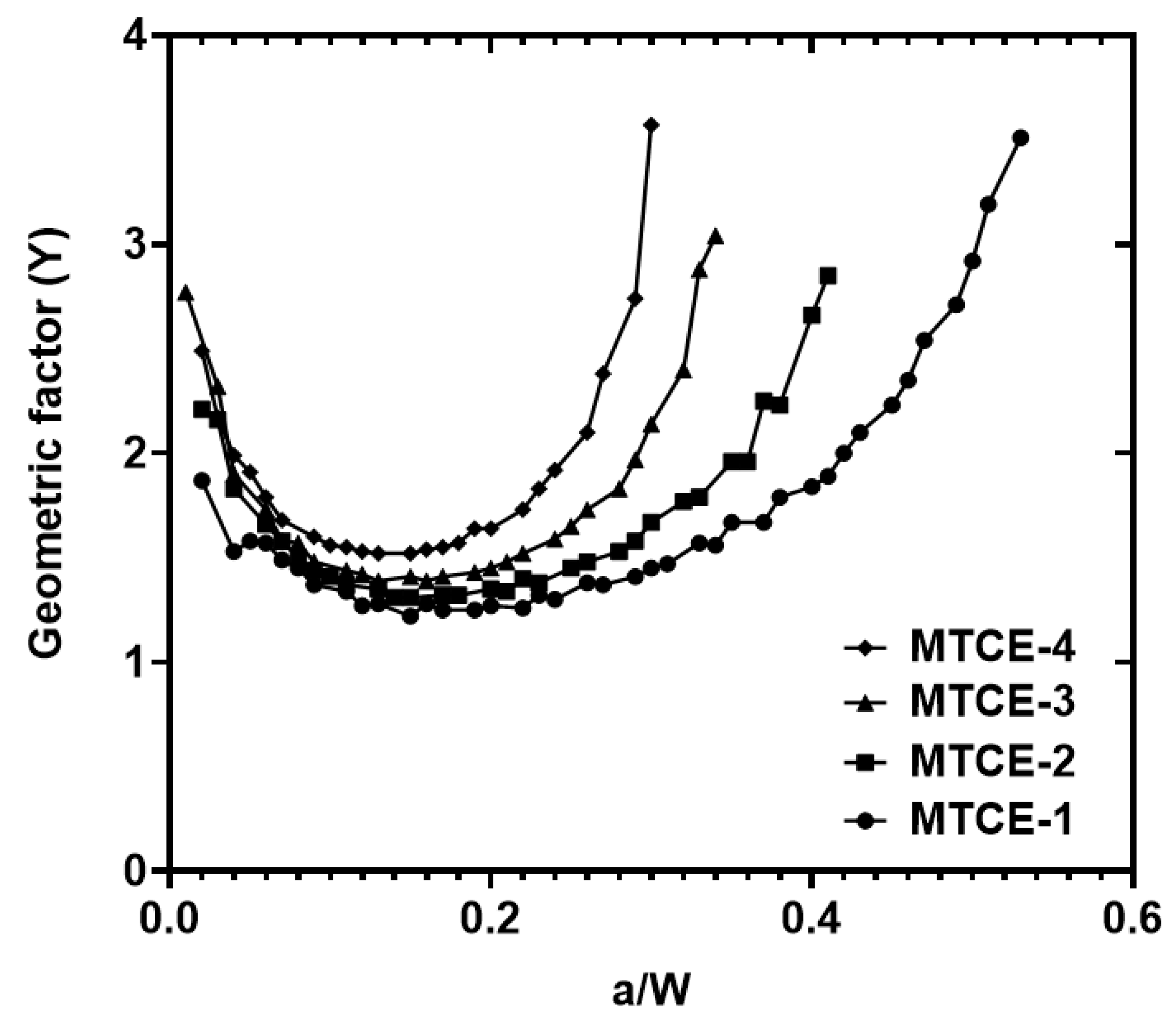
3. Results
4. Discussion
5. Conclusions
Author Contributions
Funding
Institutional Review Board Statement
Informed Consent Statement
Data Availability Statement
Acknowledgments
Conflicts of Interest
References
- Sanchez-Capa, M.; Viteri-Sanchez, S.; Burbano-Cachiguango, A. New Characteristics in the Fermentation Process of Cocoa (Theobroma cacao L.) ‘Super Á rbol’ in La Joya de los. Sustainability 2022, 14, 7564. [Google Scholar] [CrossRef]
- Gómez, E.H.; Campo, I.; Rosario, E.; Tapachula, K.C. Factores socieconómicos y parasitológicos que limitan la producción del cacao en Chiapas, México Socioeconomic and parasitological factors that limits cocoa production in Chiapas, Mexico, 2015. Rev. Mex. Fitopatol. 2015, 33, 232–246. [Google Scholar]
- Chitiva-Chitiva, L.C.; Ladino-Vargas, C.; Cuca-Suárez, L.E.; Prieto-Rodríguez, J.A.; Patiño-Ladino, O.J. Antifungal Activity of Chemical Constituents from Phytopathogen Fungi of Cocoa. Molecules 2021, 26, 3256. [Google Scholar] [CrossRef] [PubMed]
- Guerrini, A.; Sacchetti, G.; Rossi, D.; Paganetto, G.; Muzzoli, M.; Andreotti, E.; Tognolini, M.; Maldonado, M.E.; Bruni, R. Bioactivities of Piper aduncum L. and Piper obliquum Ruiz & Pavon (Piperaceae) essential oils from Eastern Ecuador. Environ. Toxicol. Pharmacol. 2009, 27, 39–48. [Google Scholar] [CrossRef]
- Guerrero, R.; Risco, G.; Cevallos, O.; Villamar, R.; Peñaherrera, S. Extractos vegetales: Una alternativa para el control de enfermedades en el cultivo de cacao (Theobroma cacao). Ing. Innovación 2020, 8, 2326. [Google Scholar] [CrossRef]
- Nairn, J.A. Direct comparison of anisotropic damage mechanics to fracture mechanics of explicit cracks. Eng. Fract. Mech. 2018, 203, 197–207. [Google Scholar] [CrossRef]
- Mecholsky, J.J. Fracture mechanics principles. Dent. Mater. 1995, 11, 111–112. [Google Scholar] [CrossRef]
- Taylor, D.; Cornetti, P.; Pugno, N. The fracture mechanics of finite crack extension. Eng. Fract. Mech. 2005, 72, 1021–1038. [Google Scholar] [CrossRef]
- Atzori, B.; Lazzarin, P.; Meneghetti, G. Fracture mechanics and notch sensitivity. Fatigue Fract. Eng. Mater. Struct. 2003, 26, 257–267. [Google Scholar] [CrossRef]
- Smith, S.M.; Scattergood, R.O. Crack-Shape Effects for Indentation Fracture Toughness Measurements. J. Am. Ceram. Soc. 1992, 75, 305–315. [Google Scholar] [CrossRef]
- Newman, J.C., Jr.; Raju, I. An empirical stress-intensity factor equation for the surface crack. Eng. Fract. Mech. 1981, 15, 185–192. [Google Scholar] [CrossRef]
- Nix, K.J.; Lindley, T.C. The Application of Fracture Mechanics to Fretting Fatigue. Fatigue Fract. Eng. Mater. Struct. 1985, 8, 143–160. [Google Scholar] [CrossRef]
- Clarke, S.M.; Griebsch, J.H.; Simpson, T.W. Analysis of Support Vector Regression for Approximation of Complex Engineering Analyses. J. Mech. Des. 2004, 127, 1077–1087. [Google Scholar] [CrossRef]
- Smola, A.J.; Scholkopf, B. A tutorial on support vector regression. Stat. Comput. 2004, 14, 199–222. Available online: http://citeseerx.ist.psu.edu/viewdoc/download;jsessionid=1CAD92EF8CCE726A305D8A41F873EEFC?doi=10.1.1.114.4288&rep=rep1&type=pdf%0Ahttp://download.springer.com/static/pdf/493/art%3A10.1023%2FB%3ASTCO.0000035301.49549.88.pdf?auth66=1408162706_8a28764ed0fae9 (accessed on 10 April 2023). [CrossRef] [Green Version]
- Heydari, M.H.; Choupani, N. A New Comparative Method to Evaluate the Fracture Properties of Laminated Composite. Int. J. Eng. 2014, 27, 991–1004. [Google Scholar] [CrossRef]
- El-Desouky, A.R. Mixed Mode Crack Propagation of Zirconia/Nickel Functionally Graded Materials. Int. J. Eng. 2013, 26, 885–894. [Google Scholar] [CrossRef]
- Guo, K.; Gou, G.; Lv, H.; Shan, M. Jointing of CFRP/5083 Aluminum Alloy by Induction Brazing: Processing, Connecting Mechanism, and Fatigue Performance. Coatings 2022, 12, 1559. [Google Scholar] [CrossRef]
- USA Department of Defense. MIL-HDBK-2097, Military Handbook: Acquisition of Support Equipment and Associated Integrated Logistics Support; USA Department of Defense: Washington, DC, USA, 1997.
- Haji, Z. Low cycle fatigue behavior of aluminum alloys AA2024-T6 and AA7020-T6. Diyala J. Eng. Sci. 2010, 127–137. [Google Scholar]
- Meggiolaro, M. Statistical evaluation of strain-life fatigue crack initiation predictions. Int. J. Fatigue 2004, 26, 463–476. [Google Scholar] [CrossRef]
- Faisal, B.M.; Abass, A.T.; Hammadi, A.F. Fatigue Life Estimation of Aluminum Alloy 2024-T4 and Fiber Glass-Polyester Composite Material. Int. Res. J. Eng. Technol. 2016, 2016, 1760–1764. Available online: www.irjet.net (accessed on 10 April 2023).
- Yang, G.; Gao, Z.L.; Xu, F.; Wang, X.G. An Experiment of Fatigue Crack Growth under Different R-Ratio for 2024-T4 Aluminum Alloy. Appl. Mech. Mater. 2011, 66–68, 1477–1482. [Google Scholar] [CrossRef]
- Hudson, M.; Scardina, J. Effect of stress ratio on fatigue crack growth in 7075-T6 Al alloy sheet. Natl. Symp. Fract. Mech. 1967. [Google Scholar]
- Wei, R.P. Fatigue-crack propagation in a high-strength. Int. J. Fract. Mech. 1968, 4, 159–168. [Google Scholar] [CrossRef]
- ANSYS. Meshing Guide; Finite Elem. Simulations Using ANSYS; Ansys: Canonsburg, PA, USA, 2015; Volume 15317, pp. 407–424. [Google Scholar] [CrossRef]
- Araque, O.; Arzola, N. Weld Magnification Factor Approach in Cruciform Joints Considering Post Welding Cooling Medium and Weld Size. Materials 2018, 11, 81. [Google Scholar] [CrossRef] [PubMed] [Green Version]
- Shawe-Taylor, J.; Cristianini, N. Kernel Methods for Pattern Analysis; Cambridge University Press: Cambridge, UK, 2004. [Google Scholar]
- Demir, S.; Toktamiş, Ö. On the adaptive Nadaraya-Watson kernel regression estimators. Hacet. J. Math. Stat. 2010, 39, 429–437. [Google Scholar]
- Fan, J.; Gijbels, I. Local Polynomial Modelling and Its Applications; Applied Pr. New York; CRC Press: Boca Raton, FL, USA, 1996. [Google Scholar]
- Chu, C.-Y.; Henderson, D.J.; Parmeter, C.F. On discrete Epanechnikov kernel functions. Comput. Stat. Data Anal. 2017, 116, 79–105. [Google Scholar] [CrossRef]
- Alshoaibi, A.M. Computational Simulation of 3D Fatigue Crack Growth under Mixed-Mode Loading. Appl. Sci. 2021, 11, 5953. [Google Scholar] [CrossRef]
- Rahmatabadi, D.; Pahlavani, M.; Bayati, A.; Hashemi, R.; Marzbanrad, J. Evaluation of fracture toughness and rupture energy absorption capacity of as-rolled LZ71 and LZ91 Mg alloy sheet. Mater. Res. Express 2018, 6, 036517. [Google Scholar] [CrossRef]


| Property | Value |
|---|---|
| Density (Kg/m3) | 2770 |
| Coefficient of thermal expansion (1/C) | 0.000023 |
| Young’s Modulus (MPa) | 71,000 |
| Poisson’s Ratio | 0.33 |
| Shear Modulus (MPa) | 26,692 |
| Bulk Modulus (MPa) | 69,608 |
| Parameter | Value |
|---|---|
| Strength Coefficient (MPa) | 714 |
| Strength Exponent | −0.078 |
| Ductility Coefficient | 0.166 |
| Ductility Exponent | −0.538 |
| Cyclic Strength Coefficient (MPa) | 502 |
| Cyclic Strain Hardening Coefficient | 0.15 |
| Constant | Value |
|---|---|
| C | 5.75 × 10⁻⁸ |
| m | 3.09 |
| Kernel Equations | |
|---|---|
| Linear | |
| Polynomial | |
| Gaussian | |
| Sigmoidal | |
| Epanechnikov | |
| Nomenclature | Greek Symbols | ||
|---|---|---|---|
| Stress Intensity Factor Mode I | Pi number | ||
| Crack length | Axial stress | ||
| Length measured from the point of grip to the end | ENW Setting Parameter | ||
| Relative crack length | Amplitude between support vectors | ||
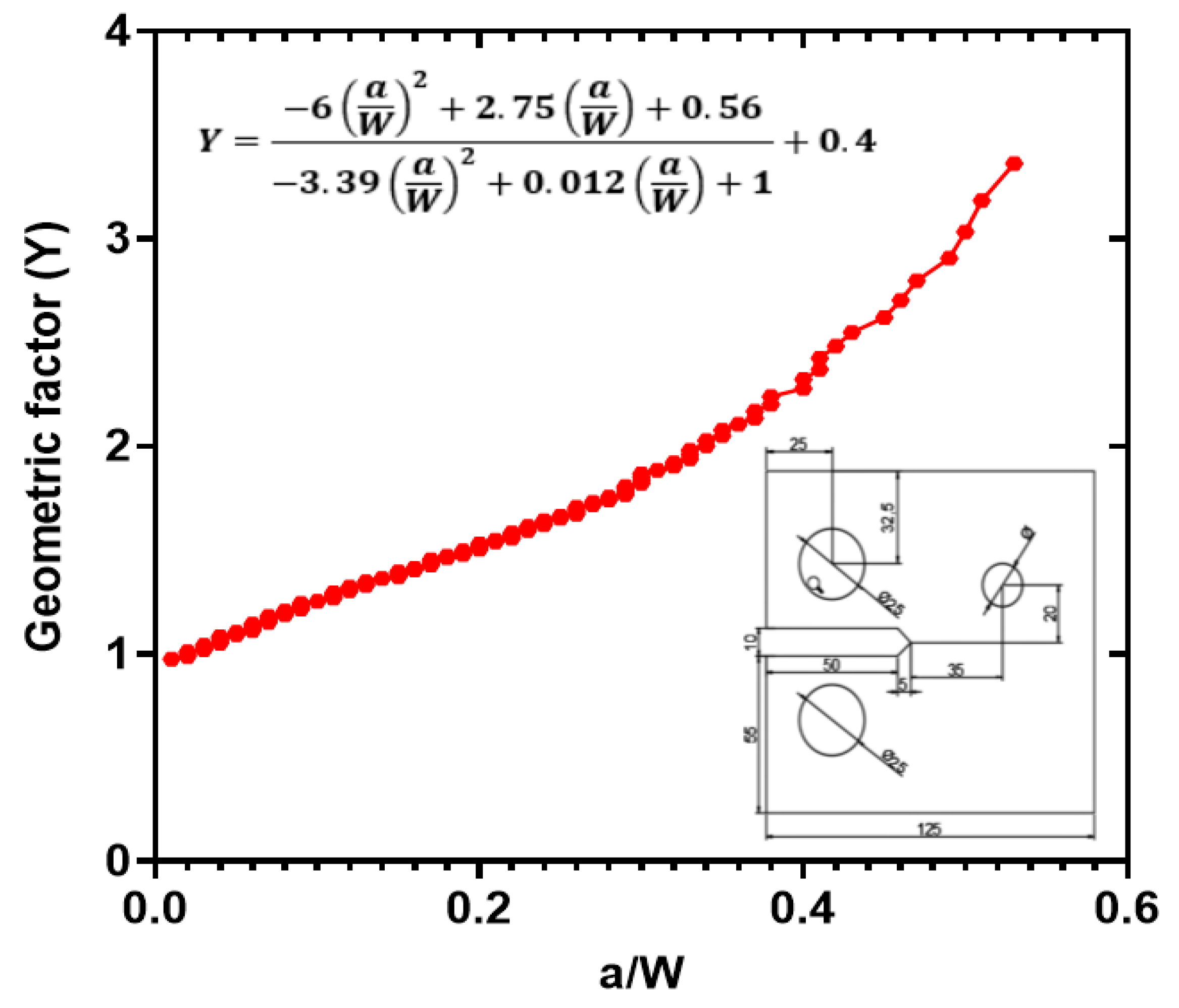
| Geometric correction factor | External margin between support vectors | ||
| Bandwidth | Arithmetic mean of data | ||
| Stress ratio | Subscripts | ||
| Kernel Equation | NWE | Nadaraya–Watson Estimator | |
| C | Paris law material constant | MTCE | Modified Tension Compact specimen |
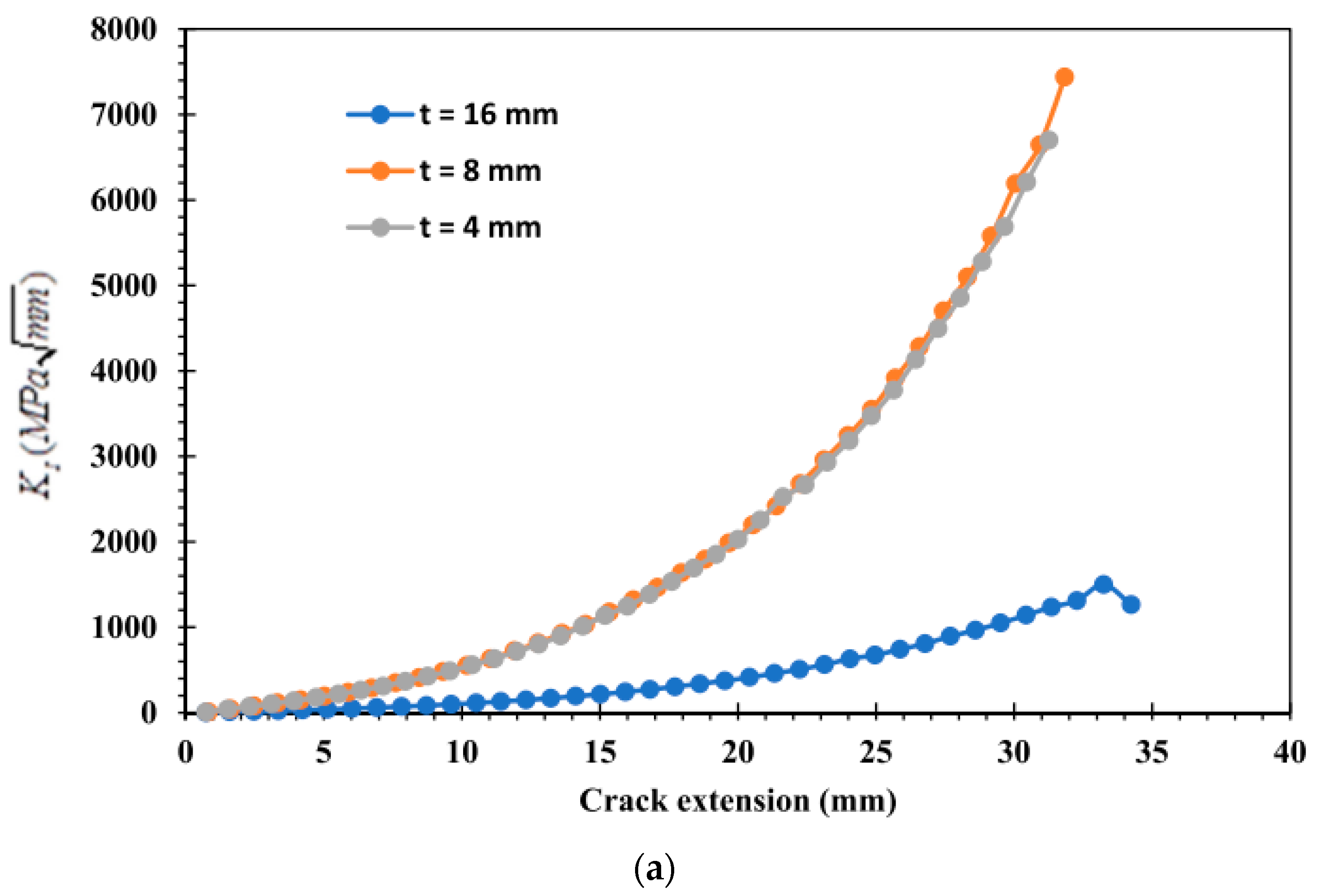
| m | Paris law material constant | SIF | Stress Intensity Factor |
| Nadaraya—Watson equation | SVR | Support Vector Regression | |
| Weight value of each vector | MSE | Mean Square Error | |
Disclaimer/Publisher’s Note: The statements, opinions and data contained in all publications are solely those of the individual author(s) and contributor(s) and not of MDPI and/or the editor(s). MDPI and/or the editor(s) disclaim responsibility for any injury to people or property resulting from any ideas, methods, instructions or products referred to in the content. |
© 2023 by the authors. Licensee MDPI, Basel, Switzerland. This article is an open access article distributed under the terms and conditions of the Creative Commons Attribution (CC BY) license (https://creativecommons.org/licenses/by/4.0/).
Share and Cite
Urrego, L.F.; García-Beltrán, O.; Arzola, N.; Araque, O. Mechanical Fracture of Aluminium Alloy (AA 2024-T4), Used in the Manufacture of a Bioproducts Plant. Metals 2023, 13, 1134. https://doi.org/10.3390/met13061134
Urrego LF, García-Beltrán O, Arzola N, Araque O. Mechanical Fracture of Aluminium Alloy (AA 2024-T4), Used in the Manufacture of a Bioproducts Plant. Metals. 2023; 13(6):1134. https://doi.org/10.3390/met13061134
Chicago/Turabian StyleUrrego, Luis Fabian, Olimpo García-Beltrán, Nelson Arzola, and Oscar Araque. 2023. "Mechanical Fracture of Aluminium Alloy (AA 2024-T4), Used in the Manufacture of a Bioproducts Plant" Metals 13, no. 6: 1134. https://doi.org/10.3390/met13061134