Article

Multi-Response Optimization of Additively Manufactured Ti6Al4V Component Using Grey Relational Analysis Coupled with Entropy Weights

1
Industrial Engineering Department, College of Engineering, Taibah University, Medinah 41411, Saudi Arabia
2
Industrial Engineering Department, College of Engineering, King Saud University, P.O. Box 800, Riyadh 11421, Saudi Arabia
*
Author to whom correspondence should be addressed.
Metals 2023, 13(6), 1130; https://doi.org/10.3390/met13061130
Submission received: 1 May 2023 / Revised: 28 May 2023 / Accepted: 14 June 2023 / Published: 16 June 2023

Abstract

:
Due to its near-net-shape manufacturing and ability to treat challenging-to-manufacture materials such as titanium alloys, Additive manufacturing (AM) is growing in popularity. However, due to the poor surface quality of AM components, finishing processes such as machining are required. One of the most difficult aspects of finishing AM components is the fact that even when using the same machining parameters, the surface roughness can vary significantly depending on the orientation of the part. In this study, electron beam melting (EBM) Ti6Al4V parts are subjected to the finishing (milling) process in three potential orientations relative to the direction of the tool feed. The impact of the feed rate, radial depth of cut, and cutting speed on the surface roughness and cutting force of the Ti6Al4V EBM part is studied while taking the orientations of the EBM components into consideration. It is found that the machined surface changes in noticeable ways with respect to orientation. A factorial design is used for the experiments, and analysis of variance (ANOVA) is used to evaluate the results. Furthermore, the grey relational analysis (GRA) method coupled with entropy weights is utilized to determine the optimal process variables for machining a Ti6Al4V EBM component. The results show that the feed rate has the greatest impact on the multi-response optimization, followed by the cutting speed, faces, and radial depth of cut.

1. Introduction

Ti6Al4V is the most extensively researched member of the family of lightweight alloys. Since the introduction of additive manufacturing (AM) techniques, titanium alloys have attracted considerable interest. Due to the advantages of additive manufacturing, its mechanical performance, and its corrosion resistance, it has found numerous applications [1]. The Ti6Al4V alloy is characterized by its high strength, low density, and high fracture toughness. Approximately 50% of all material markets recognize this alloy as the most prevalent titanium alloy. Initially, it was employed in the aircraft industry to construct intelligent aviation components. Due to the alloy’s high strength-to-weight ratio, jet engines, gas turbines, and a variety of aircraft components can all benefit from the weight reductions this material provides. In addition, its high biocompatibility with the human body has led to a variety of biomedical applications [2]. Osseointegration, corrosion protection, and specific strength all contribute to Ti6Al4V’s prominence as a medical-grade metal alloy [3,4]. However, it has a poor propensity to be machined [4], particularly when made through additive manufacturing (AM), due to its unusual microstructure, which is a function of the AM process parameters. Therefore, it is crucial to choose the appropriate cutting parameters to simultaneously decrease the cutting force and the surface roughness.
Additive manufacturing (AM) technologies provide a versatile, effective, and quick method for making complicated and individualized products [5]. One of the important techniques in AM is electron beam melting (EBM). EBM refers to a family of manufacturing methods in which materials are directly joined to create parts, typically in a layer-upon-layer fashion using 3D modeling data. The manufacturing of end-use parts with EBM is becoming increasingly common in the industry, which is hastening the development of related design, process, and manufacturing methods [6]. With the highly praised benefits of quick design-to-part transition and increased design freedoms, EBM methods continue to advance toward production-ready technologies [7]. EBM is positioned to bring about a revolution due to its innovative production model. It provides the possibility of bulk customization, flexible production, on-demand manufacturing, and decentralized production. Nonetheless, not only the complexity of manufacturing systems but also the desire for increasingly complex and high-quality products present several difficulties [8]. Poor surface quality and insufficient mechanical characteristics are also major problems for EBM processes [9].
In order to accomplish the desired material properties, tolerances, and surface finish in EBM production cycles, post-processing stages such as heat treatment and machining are often required [5]. Numerous investigations have been conducted to enhance the machinability of titanium alloy during the milling process; Iquebal et al. [10] presented the effects of Ti6Al4V EBM through machining and fine abrasive polishing. The results indicated that average surface roughness improved by 98.1% and surface hardness by 37.0%. In the case of abrasive finishing, the microhardness increased by 11% while the average surface roughness decreased by 99.82%. Gong et al. [11] demonstrated statistically significant differences in the machining behavior of Ti6Al4V across build directions in EBM specimens, as-AM, and after heat-treated laser powder bed fusion (L-PBF) specimens (21% reduced specific cutting power in L-PBF). Hojati et al. [12] studied the differences between micro-milling titanium alloy produced by selective laser melting (SLM), EBM, and conventional titanium. They tested the impact of various feeds per tooth on the surface roughness, cutting force, and burr formation. They discovered that despite EBM titanium’s greater hardness, it produced the same or lower forces. Bonaiti et al. [13] investigated the micro-milling machinability of additively manufactured Ti6Al4V by analyzing surface roughness, cutting forces, and burr formation. Comparing the AM material to the conventional titanium alloy, they discovered several differences: due to a finer microstructure, AM material exhibited higher hardness; standard titanium exhibited greater surface roughness than AM titanium; despite exhibiting increased hardness, AM titanium exhibited lower cutting forces; and standard titanium exhibited superior results when considering burr formation. Rysava and Bruschi [14] compared the micro-milling characteristics of EBM and direct metal laser sintering (DMLS) Ti6Al4V alloys based on the influence of burr formation, surface topography, surface defects, roughness, tool damage, and microstructural modifications. The results demonstrated that the most crucial cutting parameter is the feed per tooth, which directly affects the final surface roughness, the formation of burrs, and the occurrence of surface defects. In addition, they observed adhered material on the tool edges as opposed to abrasion wear and no microstructural changes. Çevik et al. [15] enhanced the surface quality of samples made from Ti6Al4V alloy using powder bed-fed additive manufacturing with various processing parameters by applying an additional process, such as CNC machining. The Ti6Al4V samples exhibited greater machinability with lower cutting forces and lower surface roughness due to the material’s rapid cooling. Yadav and Pawade [16] evaluated the compatibility and property variations of Ti6Al4V produced using AM methods (e.g., EBM, SLM, and direct energy deposition (DED)) to those produced via traditional manufacturing. According to the findings, the feed rate and the depth of cut are the most important factors in determining the presence and severity of defects (such as shallow grooves, micro-particle deposits, white layers, etc.) on the turned surfaces of Ti6Al4V alloy. SLM and DED both have almost 20% greater ultimate tensile strength and yield strength than EBM. Sartori et al. [17] investigated the turning of Ti6Al4V components manufactured by EBM and DMLS. When compared to EBM and wrought material, the DMLS-induced added characteristics demonstrated higher hardness and lower thermal conductivity. Because of this variation, spinning DMLS in dry conditions produced the deepest crater in the tool.
Some studies have shown that the 3D printing layer orientations have a substantial impact on the final appearance of the additively made components. For example, the impact of the layers’ orientations during EBM milling and turning of Ti6Al4V components and milling γ-TiAl components was investigated by [18,19,20]. The researchers discovered that different EBM component orientations during machining can result in different levels of surface roughness, even when using the same machining settings. The part orientation impact was mitigated for EBM Ti6Al4V components through heat treatment [21]. Another study [22] looked into how adjusting the layer thickness in L-PBF fabrication of stainless steel 316L parts affected milling orientations. Cozzolino et al. [23] studied the energy required to manufacture a Ti6Al4V EBM part and then turned it to achieve the desired surface roughness. The results indicate that all samples have a high surface roughness, with Ra values ranging from 27.09 to 37.95 μm in the parallel direction and from 15.66 to 34.00 μm in the perpendicular direction. After the turning process, the direction parallel to the axis of the cylindrical samples has roughness values greater than in the direction perpendicular to the axis. Moreover, Cozzolino and Astarita [24] studied the influence of the milling process parameters of EBM Ti6Al4V components in order to improve surface finishing and energy consumption. The results show that the roughness varies along the parallel direction more than the perpendicular direction due to the face. The best surface roughness is achieved by using a spindle speed of 1600 RPM and a depth of cut of 0.3 mm. Instead, although it results in somewhat higher roughness than the other process settings, the medium spindle speed (2500 rev/min) and the highest depth of cut (0.9 mm) of our experimental campaign should be chosen if minimizing overall energy consumption is the main target. While the impact of layer orientation on finishing the EBM part is known to be important, no report has been discovered to date that optimizes this effect.
Grey relational analysis (GRA) with entropy weights can solve multi-response optimization problems involving multiple criteria, and its use in multi-response problems has acquired popularity [25,26,27]. Dabwan et al. [28] applied the grey relational method with entropy weights to identify the optimal process parameters for single-point incremental forming products and found that the tool diameter has the greatest effect on the thinning of the single-point incremental forming process. She et al. [29] optimized the bending performance of optical fibers by employing grey relational analysis and discovered that the bending loss decreased by an order of magnitude. Chen et al. [30] optimized the door panel design for automobiles using Grey relational analysis and entropy weight. The results demonstrate that the optimized structure reduces the door’s weight and that the door’s performance meets the minimum requirements. It is still possible to use multi-response discrete optimization in various studies and to integrate it into manufacturing processes.
Results from various studies indicate that it is not feasible to predict how EBM processes will affect the machinability of the material and that each EBM process will have its own unique impact on the additively produced components. Therefore, more effort must be devoted to determining the impact of various EBM techniques on the machinability of the materials. The different part orientations are one of the important factors influencing EBM methods of machinability. Milling AM components while considering part orientations is difficult, but only a few studies have been devoted to tackling this issue. The purpose of this study is to analyze the effects of milling EBM Ti6Al4V components at different part orientations, feed rates, radial depths of cut, and cutting speeds on surface roughness and cutting forces, as shown in Figure 1. Furthermore, the influence of the EBM process on the machinability of Ti6Al4V is optimized using grey relational analysis coupled with entropy weights to improve the machined surface of the Ti6Al4V EBM part.

2. Materials and Methods

2.1. Material Details

Samples of Ti6Al4V were manufactured using the ARCAM EBM technique and measured 30 mm on a side, 30 mm in height, and 10 mm in depth (see Figure 2). The average particle size of the Ti6Al4V powder is 71 μm. Table 1 lists the components that compose the powdered form of Ti6Al4V. The primary EBM process parameters utilized in the fabrication of the Ti6Al4V components are listed in Table 2. The EBM variables in Table 2 were chosen based on past research, suggesting that these values were indicated by ARCAM as the default for achieving desirable microstructures and mechanical characteristics [31,32].

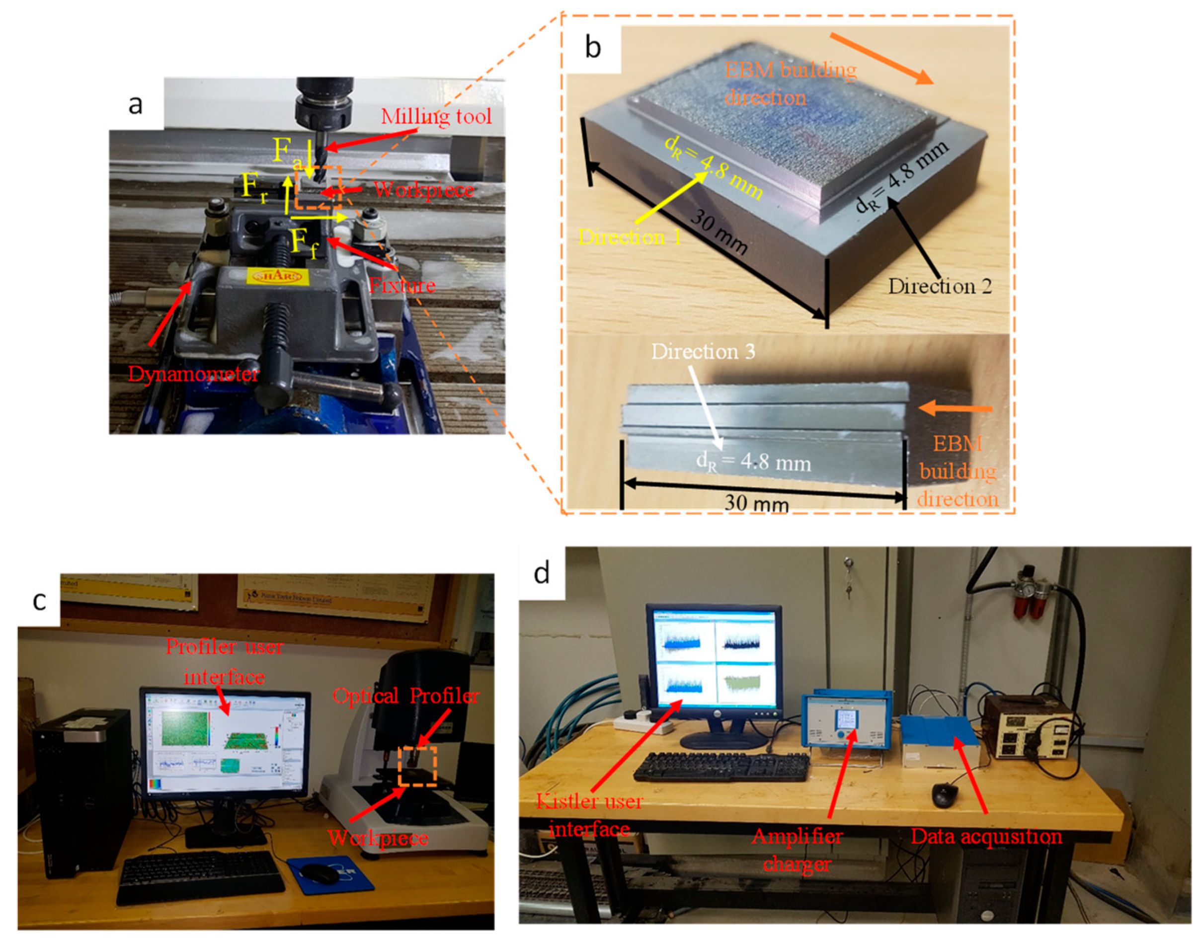
2.2. Milling Options and Measurements Setups

The faces of EBM-manufactured components have varying surface qualities. For instance, the upper surfaces of EBM Ti6Al4V components have a Sa value of 6 μm, while the side surfaces have a Sa value of 21 μm. Despite the fact that EBM components were manufactured using the optimized parameters discovered in prior research [32], the average surface roughness value on the side surfaces is still Sa = 21 μm, which is inadequate for many applications. The top and side surface roughnesses were found to be about the same (Sa = 7.5 µm and Sa = 21 µm, respectively) after employing the optimized scan methods, as reported by [34]. Therefore, an additional operation must be performed on the EBM components in order to produce a smooth surface. In this research, the conventional vertical milling method is employed for the secondary operation.
For the best possible surface finish when machining EBM components, it is essential to have the 3D-printed part oriented in the optimal fashion with regard to the tool feed direction (TFD). When milling an EBM component, the tool can be fed in one of three directions: (1) perpendicular to the layer planes (Direction 1), (2) parallel to the layer planes (Direction 2), or (3) in the layer plane itself (Direction 3). The orientations of these three parts with regard to the TFD are depicted schematically in Figure 3. The first direction is called “tool movement perpendicular to layer planes”, and it occurs when the TFD is orthogonal to the layer planes (Direction 1). The second orientation is called “tool moving parallel to layers planes”, and it occurs when the TFD is aligned to the planes of the layers being worked on (Direction 2). In the third configuration, known as “tool movement in a layer plane”, the feed path of the tool lies in the same plane as an EBM layer (Direction 3).
The milling setup is depicted in Figure 4a, and the three tool feed orientations (Direction 1, Direction 2, and Direction 3) are shown in Figure 4b for an EBM component. The samples were machined with a 30 mm/min feed rate, 10 mm tool diameter, 50 m/min cutting speed, and 0.4 mm depth of cut to smooth them out before the real experiments were performed. This was done to smooth out the rough and irregular EBM-created surfaces so they could be machined more easily. To evaluate the impact of EBM part orientation on milling quality, milling was carried out using the process settings shown in Table 3. Table 3 shows process values that are consistent with those found in prior research on machining Ti6Al4V [35,36,37].
DMG Mori’s (Oelde, Germany) DMC 635 V Ecoline vertical milling machine was used for the milling operations. 24 m/min of maximum feed rate, 1 μm of positioning accuracy, and 8000 rpm of maximum spindle speed are the specifications of this milling machine. The tool code is ISO: 1P240-1000-XA 1630 and material Id: 6259717, with a four-fluted 10 mm diameter solid carbide end mill tool having a length of 72 mm, a radial rake angle of 9°, an axial rake angle of 5.5°, and a flute helix angle of 35° from SANDVIK COROMANT. The cutting forces and the surface roughness were the two responses evaluated. Sa is a surface roughness parameter that was used to measure the degree of roughness across all three directions. The surface roughness (Sa) of the milled components was measured using a Bruker (Berlin, Germany) Contour GT-K 3D optical profilometer. ISO 25178-2 was used as the standard for filtration. After milling, the machined surface was scanned at 3 mm intervals in five distinct locations along each of the three directions (Direction 1, Direction 2, and Direction 3). The Sa was measured by measuring a 2.2 mm by 1.7 mm area at each reading, and the meaning of the five readings for each orientation was recorded. As shown in Figure 4c, during milling, the axial force (Fa), feed force (Ff), and radial force (Fr) were measured by placing the component in a fixture and then using a Kistler 5697A piezoelectric dynamometer (Kistler Instrument AG, Winterthur, Switzerland), as shown in Figure 4d. The frequency of force data sampling was 1000 Hertz. The surface morphology of the components was evaluated after the milling process using a scanning electron microscope (SEM) manufactured by Jeol, Tokyo, Japan (Model JCM 6000Plus).

2.3. Grey Relational Analysis (GRA) with Entropy Weights

This study also employs a GRA-based optimization strategy in conjunction with entropy weights to determine the optimal combination of process parameters for the machined EBM Ti6Al4V part [28,38]. GRA is one of the most intelligent decision-making methods in an industrial context; it relies on original data; provides quick and straightforward estimates; and requires minimal training or expertise to implement [39,40]. Furthermore, it has a small data size and can be effectively applied in multi-factor evaluation. The GRA strategy is exemplified below [41,42,43]. Linear normalization is a data transformation performed by GRA to make otherwise uncomparable input data fall within the range of 0 to 1. Equations (1) through (3) represent the normalized information for the ith experiment and the kth response (or quality measure).
x i * ( k ) = x i ( O ) ( k ) m i n   x i ( O ) ( k ) max   x i ( O ) ( k ) min   x i ( O ) ( k )   Higher-the-better
x i * ( k ) = m a x   x i ( O ) ( k ) x i ( O ) ( k ) max   x i ( O ) ( k ) min   x i ( O ) ( k )   Lower-the-better
x i * ( k ) = | x i ( O ) ( k ) T V | max { m a x   x i ( O ) ( k ) T V , T V min   x i ( O ) ( k ) }   Nominal-the-better   ( TV Target   Value )
Consequently, a reference sequence is determined using standardized (or comparability) sequences. The Grey Relational Coefficient (GRC) is computed by putting the normalized sequences into Equation (4).
GRC   ( x O * ( k ) , x i * ( k ) ) = m i n + ε m a x o i k + ϵ m a x
where
  • o i ( k ) represents the differences between a sequence of normal ( x i * ). Furthermore, a sequence of references ( x O * ) is denoted by the symbolization o i ( k ) , where x O * ( k ) , is the sequence of standard and x i * ( k ) the sequence between the sequence of reference x O * ( k ) , and the normalized sequence x i * ( k ) , i.e., o i ( k ) = | x O * ( k ) x i * ( k ) |is the absolute value of the difference between x O * ( k ) and x i * ( k ) .
  • m i n = min i   min k o i (k) and m a x = max i   max k o i (k), where i =1, 2,…, m and k = 1, 2, …, n.
  • ε: distinguishing coefficient, ε [0, 1].
Individual GRCs are grouped into a singular multi-response parameter during the subsequent phase. This is accomplished by assigning weights to each GRC and subsequently combining them. Individual GRC response weighting variables are analyzed using the entropy method [43]. Entropy weight calculation is a method for objectively evaluating the relative weights of responses based on their inherent information. As a result, disturbance can be reduced in the resulting weights, leading to impartial results [43,44]. This method depends on the number of data and thus reveals effective response information. The response’s larger entropy weight indicates its higher significance. Assume there are n responses and m experiments, whereas xij represents the value of ith experiment and jth response. It is possible to make a rough approximation of the entropy weight using Equations (5)–(8) [43,44].
Adjusting numbers for the ith experiment and the jth response so that they are normalized, rij
Response   of   benefit   ( higher   the   better ) = x i j x m a x
Response   of   cos t   ( smaller   the   better ) = x m i n x i j
where, (i = 1, 2, 3, 4, …, m; j = 1, 2, 3, …, n)
Entropy computation
H j = i = 1 m P i j ln   P i j ln   m   ( i   = 1 ,   2 ,   3 ,   4 ,   ,   m ;   j   = 1 ,   2 ,   3 ,   ,   n )
where, P i j = r i j i = 1 m r i j (i = 1, 2, 3, 4, …., m; j = 1, 2, 3, …, n)
Estimation of the weight of entropy
w j = 1 H j n j = 1 n H j ,   j = 1 n w j   = 1 ,   ( j   = 1 ,   2 ,   3 ,   ,   n )
Grey relational grade (GRG) is a metric that incorporates weighting with the proper GRC in each experiment. The GRG is used to evaluate the overall performance of multi-response optimization.
GRGi = k = 1 n w k GRCik
where GRGi represents the GRG for ith experiment, w k represents the weighting for the kth response, and n represents the response number. From a design of m experiments (in the present study, forty-eight), the combination of experiments with the largest GRG presents the best multi-response performance, i.e., the experiment with the largest GRG results in the process parameter configuration that generates the optimal performance.

3. Results and Discussion

The measurements and design of experiments (DOE) matrices with two replications are listed in random sequence in Table A1.

3.1. ANOVA Analysis

Analysis of variance (ANOVA) was utilized to examine the significant factors and interactions for each response. Reducing the model by removing nonsignificant (p < 0.05) variables one by one unless they are part of a significant higher-level interaction. The term with the highest p value is eliminated first, and the procedure of fitting is repeated. The ANOVA is run again, and the elimination procedure is repeated until a reduced model containing all significant terms is obtained. Table A2 presents the reduced model of an analysis of variance (ANOVA) for surface roughness (Sa), which reveals that the variables Face, cutting speed (V), feed rate (f), and radial depth of cut (Rd) have a significant effect on the output, which are consistent with those found by [19,21]. There is a considerable effect on the Sa from two-source interactions such the Face and V, Face and f, Face and Rd, V and f, and V and Rd. Moreover, three-source interactions, including Face, V, and f, Face, V, and Rd, and Face, f, and Rd, have significant effects on the Sa. The R-square, adjusted R-square, and predicted R-square values presented in Table A2 indicate that the model terms provide an outstanding representation of the data variability.
Table A3 displays the findings of an ANOVA for radial force (Fr), which reveals that the variables Face, Feed rate (f), and Radial depth of cut (Rd) have a significant effect on output, as reported by [19]. There is a significant effect on the Sa from two-source interactions such the Face and f, V and f, and f, and Rd. Moreover, three-source interactions, including V, f, and Rd have significant effects on the Sa. The R-square, adjusted R-square, and predicted R-square values presented in Table A3 indicate that the model terms provide an outstanding representation of the data variability.
The ANOVA results for Feed force (Ff) presented in Table A4 indicate that Feed rate (f) and Radial depth of cut (Rd) have a significant effect on output. Only one significant effect on the Sa from two-source interactions including V and f was found. Moreover, three-source interactions, including Face, V, and F and V, f and Rd have significant effects on the Sa. The R-square, adjusted R-square, and predicted R-square values presented in Table A4 indicate that the model terms provide an outstanding representation of the data variability.
Table A5’s ANOVA results for Axial force (Fa) indicate that Cutting speed (V) and Feed rate (f) have a significant effect on output, as reported by [45]. There is a significant effect on the Sa from two-source interactions such the V and Rd, and f and Rd. Moreover, three-source interactions, including Face, V, and f and V, f, and Rd have significant effects on the Sa. The R-square, adjusted R-square, and predicted R-square values presented in Table A5 indicate that the model terms provide an outstanding representation of the data variability.

3.2. Grey Relational Analysis (GRA) with Entropy Weights Analysis

As a first step in the GRA implementation, the experimental findings from Table A1 are normalized between 0 and 1 under the lower-the-better condition using Equation (2). Both the reference sequence xO*(k) and the standardized or comparability sequence xi*(k) (k) are given to response quantities. After cleaning the data, an overview of all sequences can be found in Table A6. As stated by Deng (1989) [46], a higher number of normalized values correlates with optimal performance and, consequently, shows greater efficacy.
The deviation sequences Δ01(k) in Table A7, can be obtained as follows.
Δ01(1) = |xO*(1) − x1*(1)| = |1 − 0.5734| = 0.4266
Δ01(2) = |xO*(2) − x1*(2)| = |1 − 0.2320| = 0.7680
Δ01(3) = |xO*(3) − x1*(3)| = |1 − 0.2319| = 0.7681
Δ01(4) = |xO*(4) − x1*(4)| = |1 − 0.0503| = 0.9497
therefore, Δ01 = (0.4266, 0.7680, 0.7681, 0.9497).
Results for all Δ0i for i = 1, …., 48 are shown in Table A7 and the same calculation method is used for i = 2, 3, 4, …, 48.
By analyzing the data in Table A8, Δmin (k) and Δmax (k) can be defined as follows.
Δmin = Δ021 (1) = Δ021 (2) = Δ032 (3) = 0.0000
Δmax = Δ026 (1) = Δ018 (2) = Δ018 (3) = 1.0000
Differentiating coefficient integration ε = 0.5 into Equation (6) yields the GRC for each response.
Listed below are examples of the GRCi (k) approximation.
GRC 1   ( 1 ) = 0.0000 + 0.5 × ( 1.0000 ) 0.4266 + 0.5 × ( 1.0000 ) = 0.5396
GRC 1   ( 2 ) = 0.0000 + 0.5 × ( 1.0000 ) 0.7680 + 0.5 × ( 1.0000 ) = 0.3943
GRC 1   ( 3 ) = 0.0000 + 0.5 × ( 1.0000 ) 0.7681 + 0.5 × ( 1.0000 ) = 0.3943
GRC 1   ( 4 ) = 0.0000 + 0.5 × ( 1.0000 ) 0.9497 + 0.5 × ( 1.0000 ) = 0.3449
Hence, GRC1(k) = (0.5396, 0.3943, 0.3943, 0.3449), k = 1, 2, 3. The same steps are taken for i = 2, 3, 4, …., 48. Table A8 illustrates the GRC for every experiment conducted.
Weights for every measure of performance must be known in order to optimize a problem with numerous responses. Expertise and trial-and-error are highly reliant on the traditional method of evaluating the values of each response, leading to a rise in decision-making uncertainty. Entropy is introduced as a technique for dispassionately assessing the significance of each response in GRA. The GRC of each quality measure is represented by an element in Table A6 of the array Multiple Quality Characteristics (MQC). The estimated weights in Equations (4)–(7) are calculated using this data.
The GRG of the experiments’ comparability sequence can be obtained as shown in Table A9.
Based on the experimental design, Table A9 reveals that the machining of Ti6Al4V experiment number 19 has the highest GRG. Consequently, experiment number 19 determines the optimal multi-response parameter from the 48 experiments.
The average GRG for each parameter level is calculated to identify the best set of processing variables for enhanced usefulness. This procedure clusters the GRGs based on the process parameter levels in each column, then averages the parameters with the same parameter levels. For example, for the factor faces (Table A1), experiments 1, 2, 3, 4, 5, 6, 7, 8, 25, 26, 27, 28, 29, 30, and 32 are adjusted to level 1. Consequently, the average GRG for A1 can be determined by analyzing the data in Table A10:
A 1 = 0.41828 + 0.56443 + 0.7633 + 0.58548 + + 0.61729 + 0.64201 + 0.66599 16 = 9.612681073 16 = 0.600793
Both A2 and A3 are predicted to have average GRGs of 0.56073 and 0.565408, respectively.
Each level of machining parameter is computed using the same procedure, and Table A10’s main effect analysis is performed.
Figure 5 demonstrates that the various responses of the machining of the EBM Ti6Al4V component are influenced by changes to the process variables. The selection in faces (Direction 1) and decrease in radial depth of cut increases the GRGs, leading to a decrease in surface roughness and cutting forces which are consistent with [19,20,21]. However, as cutting speed and feed rate decrease from a greater to a lesser value, the relational grades for the output characteristics diminish. This indicates that increased cutting speed and feed rate are essential for minimizing surface roughness and cutting force. Changes from level 1 to level 2 and level 3 in faces have a significant influence on surface roughness and cutting force. The surface morphology of milled Ti6Al4V EBM in three directions is shown in Figure 6. Scanning electron micrographs (SEM) reveal various tool feed marks. The prominent tool feed marks are generated when the milling tool is moved parallel to the layers’ planes, which impart larger roughness on the surface after machining, as shown in Figure 6c. While the thick tool feed marks are generated when the interfaces between successive layers are perpendicular to the tool feed direction, leading to large surface roughness, as shown in Figure 6b. Furthermore, the minor tool feed marks are generated when the milling tool is moved perpendicular to the layers, which achieved a smaller surface roughness, as shown in Figure 6a. All of this is consistent with [19,20,21,22].
The difference in surface roughness among the three directions is because the tool interacts with a single EBM layer while machining along Direction 3 and exerts compressive forces at the EBM layer interface, which causes the bonded layers to rupture, resulting in a high surface roughness. In contrast, if the tool is fed in Direction 1, it interacts/cuts the group of layers with radial depth while exerting force on the layer bonds/interfaces, thereby preventing the tearing of adjacent layers. The layer interfaces still experience tensile stresses when Direction 2 is employed, and bond breaking may take place as the tool is fed throughout the layer group. This contributes to Direction 2’s mild roughness. Figure 7 shows the differences in 3D surface topography characterizations extracted along Direction 1, Direction 2, and Direction 3.
Regarding the cutting forces, when machining is conducted in Direction 1, the tool interacts with a group of EBM-bonded layers without causing tensile stresses at the interfaces of the layers. This results in different cutting forces in Direction 1 compared to Direction 3, in which the tool passes/cuts a single EBM layer while exerting maximal tensile forces on the interfaces, resulting in the lowest machining resistance. On the other hand, in Direction 2, the tool traverses multiple layers covered by the radial depth of cut. However, the interfaces of the layers are still subjected to tearing forces, which degrade the material for cutting, and intermediate cutting forces are generated. The results of surface morphology, roughness, and cutting forces are consistent with the result of GRG.
Therefore, by choosing the parameter level with the highest GRG (level 1 in faces, level 2 in cutting speed, level 1 in feed rate, and level 1 in the radial depth of cut; Figure 5), the optimal combination of process parameters can be easily derived from the main effect analysis. The optimal parameter settings that produce the lowest surface roughness and cutting force for machined EBM Ti6Al4V parts are predicted to be level 1 for faces, feed rate, and radial depth of cut, and level 2 for cutting speed.
The level-wise GRG (Figure 5) demonstrates the change in the multi-response as the process parameters progress from levels one to levels two and three. Comparing the values in the final column of Table A10, the difference between the minimum and maximum GRG values for factor feed rate is clearly the greatest, followed by factors cutting speed, faces, and radial depth of cut. This demonstrates that the feed rate has the greatest impact on multi-response optimization, followed by cutting speed, faces, and radial depth of cut.

4. Conclusions

This study demonstrates the value of careful process parameter control in the milling of Ti6Al4V components made through the EBM process. This study firmly establishes the significance and impact of controlling process factors on a finished machined surface. Improved surface roughness and less cutting force are two outcomes of this study’s work on the Ti6Al4V EBM component. Furthermore, the effect of milling parameters on the part orientation of the Ti6Al4V EBM component is optimized using the grey relational analysis (GRA) technique with entropy weights.
The following are the main points of conclusion:
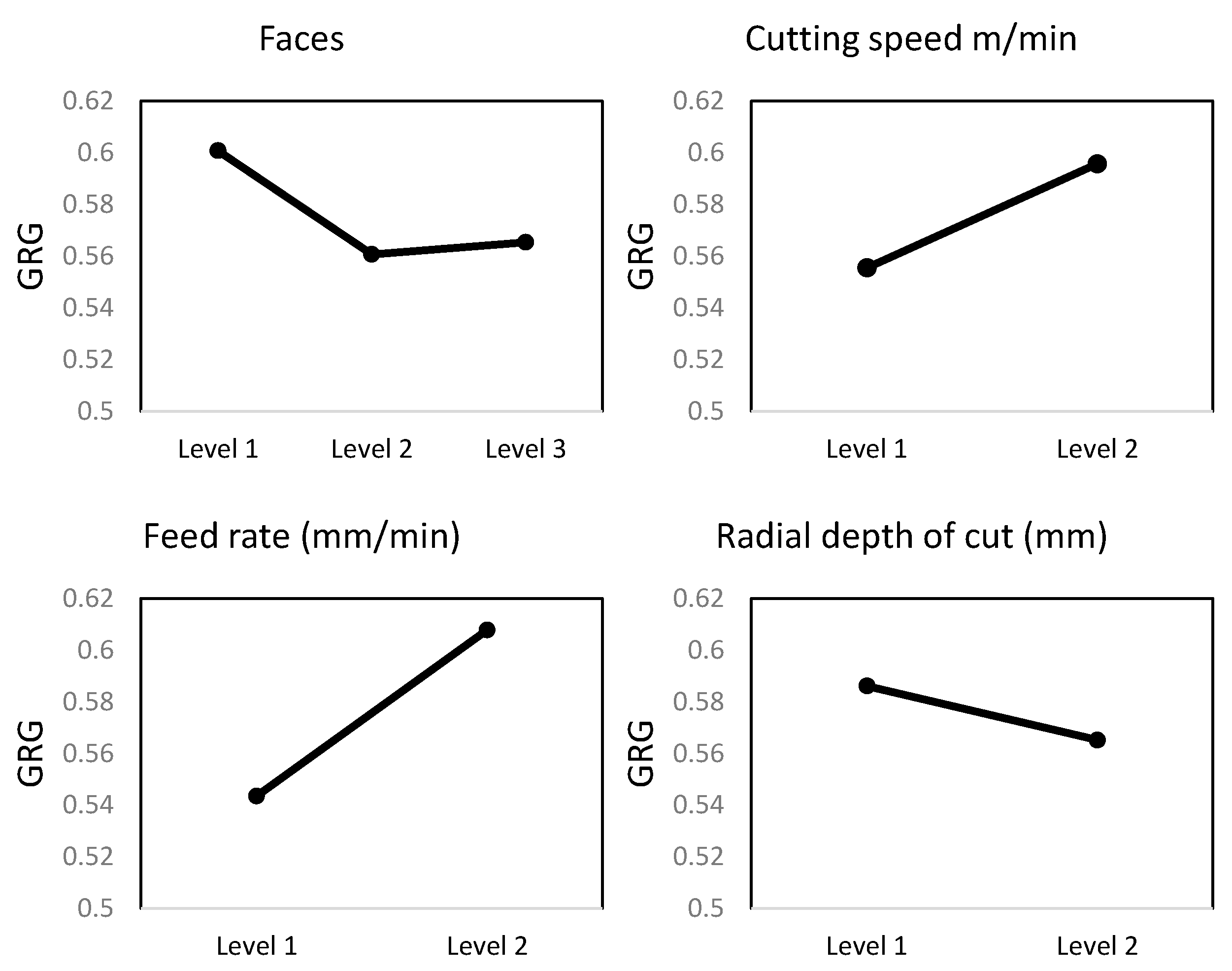
  • Feed rate is the most important component when assessing surface roughness and cutting force regarding the milling process for the Ti6Al4V EBM part.
  • Cutting speed is the second factor that affects the surface roughness and cutting force for the milling performance of the Ti6Al4V EBM part.
  • The selection of the direction of layer orientation in the EBM part has a significant effect during the milling process to achieve minimum surface roughness and cutting force.
  • The radial depth of cut is the lowest effect factor during the milling process for the Ti6Al4V EBM part.
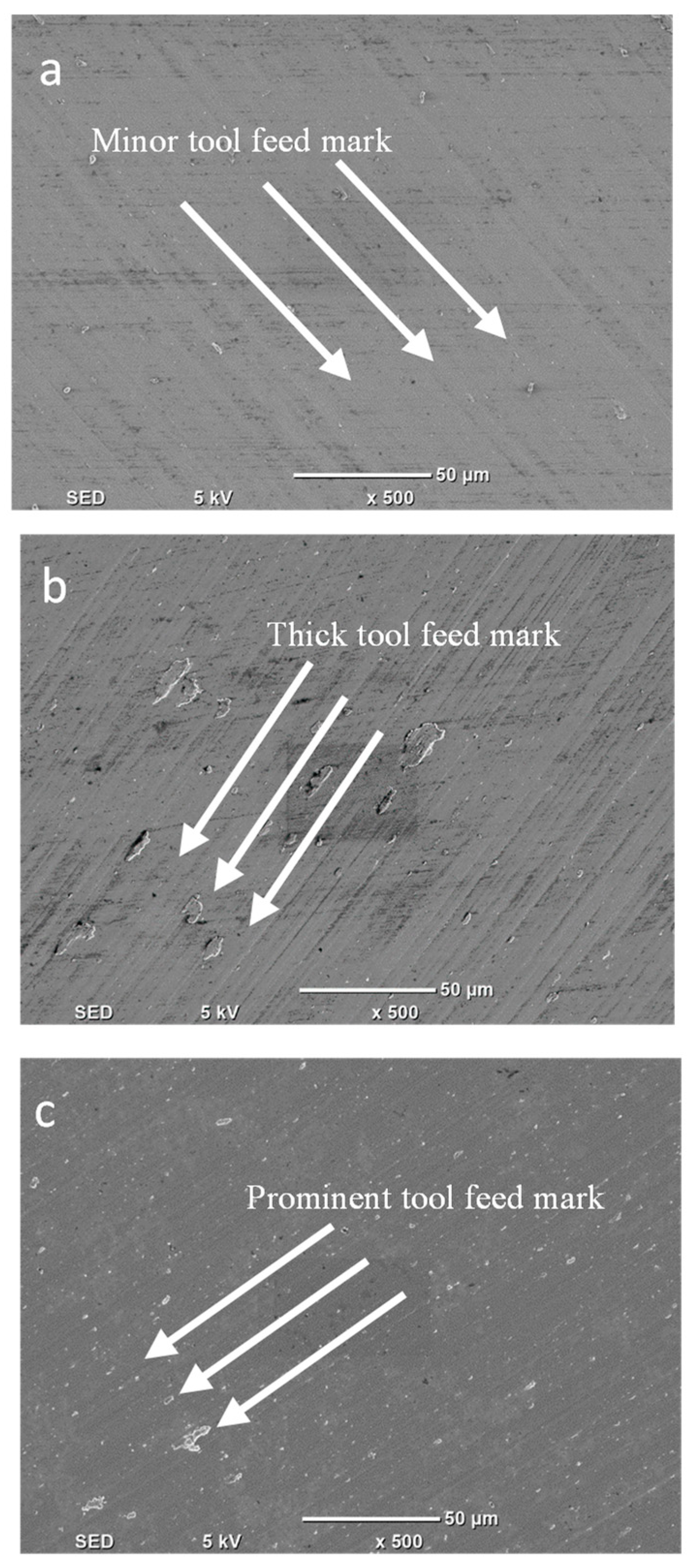
  • The study also concludes that the part orientation effect is likely one of the most important factors governing the surface roughness and surface morphology of the machined EBM Ti6Al4V component.
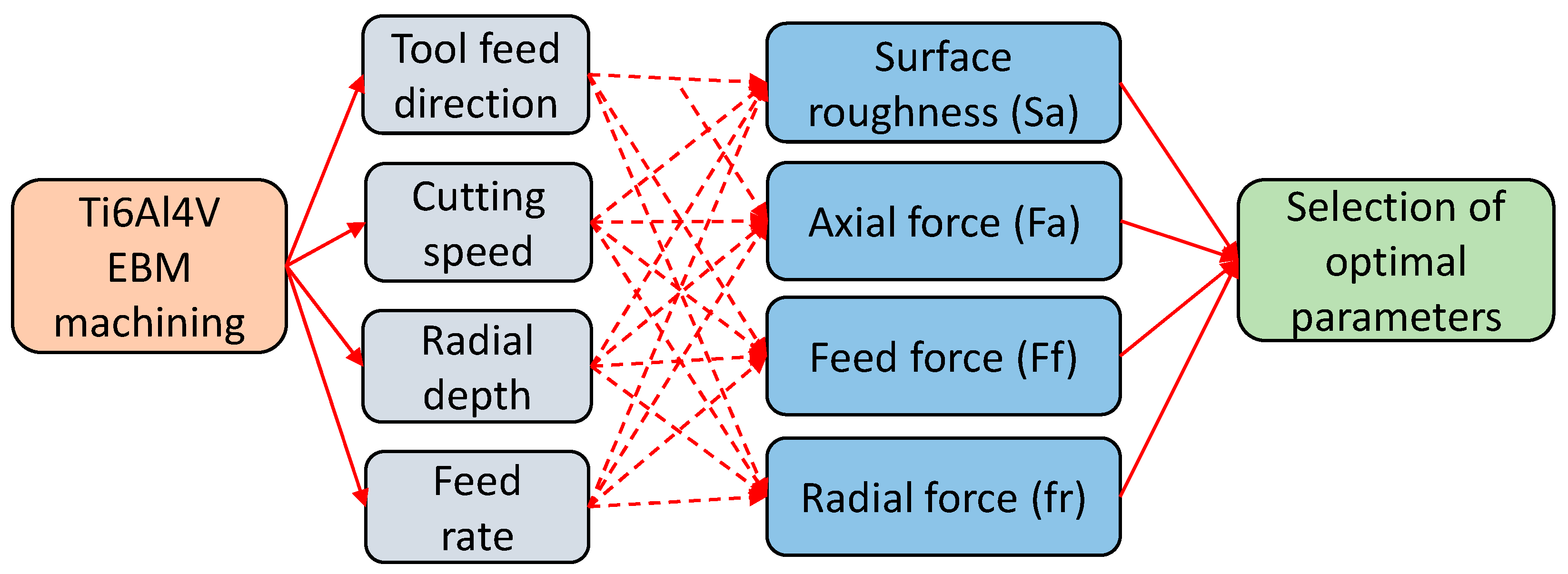
  • The multi-response optimization (GRA-Entropy) shows that the optimal machining efficiency of a Ti6Al4V EBM component can be achieved if the component is machined in direction 1 at a feed rate of 60 mm/min, a cutting speed of 80 m/min, and a radial depth of cut of 2.4 mm.

Author Contributions

Conceptualization, A.D., S.A. and A.M.A.-S.; methodology, A.D. and H.K.; validation, A.D. and E.H.A.; formal analysis, A.D. and K.N.A.; investigation, A.D., S.A. and A.M.A.-S.; data curation, A.D., E.H.A., H.K. and K.N.A.; writing—original draft preparation, A.D.; writing—review and editing, S.A., A.M.A.-S., K.N.A. and E.H.A.; visualization, A.D.; supervision, S.A. and A.M.A.-S.; resources, K.N.A. and E.H.A. All authors have read and agreed to the published version of the manuscript.

Funding

Researchers Supporting Project number (RC442/50), Taibah University, Medinah, Saudi Arabia.

Data Availability Statement

All data generated or analyzed during this study are included in the present article.

Acknowledgments

The authors extend their appreciation to, Taibah University, represented by the Deanship of Scientific Research, for funding this project No. (RC-442/50).

Conflicts of Interest

The authors declare no conflict of interest.

Appendix A

Table A1. DOE matrix and corresponding results.
9Input ParametersResponses
FacesV (m/min)f (mm/min)Rd (mm)Sa (μm)Fr (N)Ff (N)Fa (N)
1C50302.40.145147.173.02177.3
2B50302.40.193102.899.63173.2
3A50302.40.14790.0488.6171.5
4A50302.40.148114.178170
5A80304.80.11431.6885.46154.6
6A80304.80.11641.6682.59152.6
7B50602.40.1426.2146.12152.6
8C50302.40.144139.360.23149.1
9B50604.80.15665.7872.51138.7
10A80604.80.14620.0374.06137.9
11C80604.80.12765.6554.63126.1
12B80304.80.13649.2980.35123.5
13C50304.80.17756.1155.17119.7
14B80604.80.15720.7161.41119.4
15B80304.80.1379.7577.08118.3
16B80302.40.17564.249.17117.9
17B80602.40.15964.249.17117.9
18B50602.40.1319.0748.81117.6
19C50304.80.18649.755.07117.2
20C80302.40.17865.9548.88109.2
21C50604.80.17961.0245.88106.6
22C50604.80.18258.0945.18106.4
23C80304.80.15247.2248.9104.4
24C80604.80.147.91645.1103.9
25B50604.80.15458.6450.47103.8
26B50304.80.15421.4145.55102.4
27A50304.80.17334.2353.66102.3
28B50302.40.18960.0750.63102
29A50604.80.15711.2252.14101.2
30A50604.80.16515.0750.5399.89
31A50304.80.16529.5546.0494.71
32C80602.40.15254.2567.9588.59
33A80602.40.16450.553.7776.64
34B50304.80.14638.7641.4374.52
35C80602.40.15435.957.4474.49
36C80304.80.15141.2339.1173.74
37A50602.40.13511.7214.8472.74
38A50602.40.13222.3827.6671.54
39B80602.40.1649.2136.9371.49
40A80604.80.13644.0126.267.06
41A80302.40.12775.4539.5861.4
42A80602.40.16129.5840.6150.86
43B80302.40.16513.3321.9346.41
44A80302.40.12724.627.1943.66
45B80604.80.15737.6219.2743.14
46C80302.40.17556.9816.3936.98
47C50602.40.1916.7556.37832.22
48C50602.40.1884.89511.0731.37
Table A2. ANOVA results for Sa.
SourceDFSeq SSAdj SSAdj MSF-Valuep-Value
Model200.017480.017480.00087417.020
Face20.0030460.0030460.00152329.670
V10.0020230.0020230.00202339.40
f10.0000010.0000010.0000010.020.898
Rd10.0002950.0002950.0002955.740.024
Face*V20.0007130.0007130.0003566.940.004
Face*f20.0007620.0007620.0003817.420.003
Face*Rd20.0007080.0007080.0003546.90.004
V*f10.0002690.0002690.0002695.240.03
V*Rd10.0023670.0023670.00236746.110
f*Rd10.000190.000190.000193.710.065
Face*V*f20.0041620.0041620.00208140.540
Face*V*Rd20.0006770.0006770.0003386.590.005
Face*f*Rd20.0022670.0022670.00113422.080
R-sq = 92.65%, R-sq (adj) = 87.21%, R-sq(pred) = 76.78%.
Table A3. ANOVA results for Fr.
SourceDFSeq SSAdj SSAdj MSF-Valuep-Value
Model1138,179.438,179.43470.8610.610
Face22411.92411.91205.933.690.035
V1946.8946.8946.762.890.098
f17354.67354.67354.6122.480
Rd13045.63045.63045.649.310.004
Face*f22268.32268.31134.173.470.042
V*f15432.25432.25432.1716.60
V*Rd147.147.147.130.140.707
f*Rd1812581258125.0424.830
V*f*Rd18547.98547.98547.9126.120
R-sq = 76.42%, R-sq (adj) = 69.22%, R-sq(pred) = 58.08%.
Table A4. ANOVA results for Ff.
SourceDFSeq SSAdj SSAdj MSF-Valuep-Value
Model1514,20414,204946.934.580
Face2556.7556.7278.371.350.274
V1554.980.020.878
f11944.41944.41944.399.410.004
Rd1782.8782.8782.773.790.06
Face*V2282.6282.6141.310.680.512
Face*f2341.6341.6170.820.830.447
V*f11253.61253.61253.566.070.019
V*Rd1649649649.033.140.086
f*Rd1131.7131.7131.680.640.431
Face*V*f219411941970.494.70.016
V*f*Rd16315.66315.66315.6230.560
R-sq = 68.23%, R-sq (adj) = 53.34%, R-sq(pred) = 28.52%.
Table A5. ANOVA results for Fa.
SourceDFSeq SSAdj SSAdj MSF-Valuep-Value
Model1543,930.143,930.12928.73.420.002
Face2860.6860.6430.30.50.61
V14572457245725.330.028
f14894.94894.94894.95.710.023
Rd11578.91578.91578.91.840.184
Face*V22502501250.150.865
Face*f22738.62738.61369.31.60.218
V*f12616.12616.12616.13.050.09
V*Rd17079.67079.67079.68.260.007
f*Rd12088208820882.440.128
Face*V*f26908.46908.43454.24.030.027
V*f*Rd110,343.110,343.110,343.112.070.001
R-sq = 61.56%, R-sq (adj)= 43.54%, R-sq(pred) = 13.51%.
Table A6. The Resulting Sequences of Data Preprocessing.
RunSa (μm)Fr (N)Ff (N)Fa (N)
10.57340.23200.23190.0503
20.36220.82670.57470.5659
30.73810.95200.90920.7165
40.35800.92840.52650.5305
50.83530.50390.64400.7942
60.97470.74150.18270.1692
70.37490.67940.49180.6898
80.59450.89360.27420.2702
90.06020.61210.52550.5157
100.59870.76190.62420.7043
110.64940.99080.57380.1696
120.47200.57190.29080.2647
130.22700.58300.54120.4074
140.72970.68790.20680.3689
150.42980.58300.54120.4074
160.46360.88880.40980.3967
170.62410.05510.42260.1933
180.20170.63990.47680.3946
190.02850.98691.00000.9941
200.18060.60540.57640.4848
210.18900.57070.54430.4666
220.53960.74450.64900.7096
230.52270.65300.33980.6079
240.83530.57290.48260.3506
250.58610.40130.11830.0394
260.26080.79380.49300.5137
270.77610.87710.77180.7247
280.45930.95550.50920.5218
290.84370.86150.77680.9158
301.00000.81170.15190.1554
310.41290.82640.63290.8664
320.72540.72500.78750.7554
330.00000.31130.00000.0284
340.50160.88390.58000.5131
350.78880.97060.54500.4090
360.49740.62220.52710.5039
370.36220.94070.83330.8969
380.71700.96590.24180.4046
390.42130.68840.67240.7250
400.45510.76990.86170.9193
410.61770.00000.28540.0000
420.09190.68500.47780.4120
430.06651.00000.94971.0000
440.14260.62600.58390.4860
450.22700.63380.89260.9616
460.52690.70240.54400.4997
470.50160.78200.45250.7045
480.67480.97880.58480.5032
Table A7. Deviation sequences.
RunSa (μm)Fr (N)Ff (N)Fa (N)
10.42660.76800.76810.9497
20.63780.17330.42530.4341
30.26190.04800.09080.2835
40.64200.07160.47350.4695
50.16470.49610.35600.2058
60.02530.25850.81730.8308
70.62510.32060.50820.3102
80.40550.10640.72580.7298
90.93980.38790.47450.4843
100.40130.23810.37580.2957
110.35060.00920.42620.8304
120.52800.42810.70920.7353
130.77300.41700.45880.5926
140.27030.31210.79320.6311
150.57020.41700.45880.5926
160.53640.11120.59020.6033
170.37590.94490.57740.8067
180.79830.36010.52320.6054
190.97150.01310.00000.0059
200.81940.39460.42360.5152
210.81100.42930.45570.5334
220.46040.25550.35100.2904
230.47730.34700.66020.3921
240.16470.42710.51740.6494
250.41390.59870.88170.9606
260.73920.20620.50700.4863
270.22390.12290.22820.2753
280.54070.04450.49080.4782
290.15630.13850.22320.0842
300.00000.18830.84810.8446
310.58710.17360.36710.1336
320.27460.27500.21250.2446
331.00000.68871.00000.9716
340.49840.11610.42000.4869
350.21120.02940.45500.5910
360.50260.37780.47290.4961
370.63780.05930.16670.1031
380.28300.03410.75820.5954
390.57870.31160.32760.2750
400.54490.23010.13830.0807
410.38231.00000.71461.0000
420.90810.31500.52220.5880
430.93350.00000.05030.0000
440.85740.37400.41610.5140
450.77300.36620.10740.0384
460.47310.29760.45600.5003
470.49840.21800.54750.2955
480.32520.02120.41520.4968
Table A8. GRC for forty-eight comparability sequences.
RunSa (μm)Fr (N)Ff (N)Fa (N)
10.53960.39430.39430.3449
20.43940.74260.54040.5353
30.65630.91240.84630.6382
40.43780.87480.51360.5157
50.75220.50200.58410.7084
60.95180.65920.37960.3757
70.44440.60930.49590.6171
80.55220.82450.40790.4066
90.34730.56310.51310.5080
100.55480.67740.57090.6284
110.58780.98180.53990.3758
120.48640.53870.41350.4047
130.39280.54530.52150.4576
140.64910.61570.38660.4421
150.46720.54530.52150.4576
160.48240.81810.45860.4532
170.57080.34600.46410.3826
180.38510.58130.48860.4523
190.33980.97451.00000.9884
200.37900.55890.54130.4925
210.38140.53810.52320.4838
220.52060.66180.58760.6326
230.51160.59030.43090.5605
240.75220.53930.49150.4350
250.54710.45510.36190.3423
260.40350.70800.49650.5069
270.69070.80260.68660.6449
280.48050.91830.50470.5111
290.76190.78300.69130.8558
301.00000.72640.37090.3719
310.45990.74230.57660.7892
320.64550.64520.70170.6715
330.33330.42060.33330.3398
340.50080.81150.54350.5066
350.70300.94450.52360.4583
360.49870.56960.51390.5020
370.43940.89400.74990.8291
380.63860.93610.39740.4564
390.46350.61610.60420.6452
400.47850.68480.78330.8611
410.56670.33330.41170.3333
420.35510.61350.48920.4595
430.34881.00000.90851.0000
440.36830.57210.54580.4931
450.39280.57720.82320.9286
460.51380.62690.52300.4999
470.50080.69640.47730.6285
480.60590.95920.54630.5016
Table A9. The grey relational grade and its rank.
RunGRGRank
10.4182846
20.5644325
30.76334
40.5854822
50.6366613
60.5915620
70.5416729
80.5477828
90.4828538
100.6078616
110.6213414
120.4608443
130.4792841
140.5233632
150.4978835
160.5530927
170.4408944
180.4768642
190.825681
200.4929337
210.4816139
220.6006619
230.5233333
240.5544826
250.426645
260.5287331
270.706246
280.6036418
290.773013
300.6172915
310.6420112
320.665999
330.3567748
340.5905921
350.6573610
360.5210434
370.72815
380.6071217
390.5822423
400.701957
410.4112647
420.4793240
430.814332
440.4948236
450.680458
460.5408930
470.5757624
480.6532611
Table A10. Calculation of GRGs main effects.
ParametersLevel 1Level 2Level 3Max-Min
Faces0.6007930.560730.5654080.040062
Cutting speed m/min 0.5554770.59581-0.040334
Feed rate (mm/min)0.5435180.60777-0.064251
Radial depth of cut (mm)0.5861220.56517-0.020956

References

  1. Ghio, E.; Cerri, E. Additive Manufacturing of AlSi10Mg and Ti6Al4V Lightweight Alloys via Laser Powder Bed Fusion: A Review of Heat Treatments Effects. Materials 2022, 15, 2047. [Google Scholar] [CrossRef] [PubMed]
  2. Torino, P.D.I. Characterization of Powder and Its Bulk Ti-6Al-V Samples Produced by Electron Beam Melting Process. Master’s Thesis, Polytechnic University, Bari, Italy, 2019. [Google Scholar]
  3. Murr, L.E.; Quinones, S.A.; Gaytan, S.M.; Lopez, M.I.; Rodela, A.; Martinez, E.Y.; Hernandez, D.H.; Martinez, E.; Medina, F.; Wicker, R.B. Microstructure and Mechanical Behavior of Ti-6Al-4V Produced by Rapid-Layer Manufacturing, for Biomedical Applications. J. Mech. Behav. Biomed. Mater. 2009, 2, 20–32. [Google Scholar] [CrossRef] [PubMed]
  4. Özel, T.; Thepsonthi, T.; Ulutan, D.; Kaftanoglu, B. Experiments and Finite Element Simulations on Micro-Milling of Ti–6Al–4V Alloy with Uncoated and CBN Coated Micro-Tools. CIRP Ann.-Manuf. Technol. 2013, 60, 85–88. [Google Scholar] [CrossRef]
  5. Gong, X.; Zeng, D.; Groeneveld-Meijer, W.; Manogharan, G. Additive Manufacturing: A Machine Learning Model of Process-Structure-Property Linkages for Machining Behavior of Ti-6Al-4V. Mater. Sci. Addit. Manuf. 2022, 1, 6. [Google Scholar] [CrossRef]
  6. Grierson, D.; Rennie, A.E.W.; Quayle, S.D. Machine Learning for Additive Manufacturing. Encyclopedia 2021, 1, 576–588. [Google Scholar] [CrossRef]
  7. Oyelola, O.; Crawforth, P.; M’Saoubi, R.; Clare, A.T. Machining of Additively Manufactured Parts: Implications for Surface Integrity. Procedia CIRP 2016, 45, 119–122. [Google Scholar] [CrossRef]
  8. Qin, J.; Hu, F.; Liu, Y.; Witherell, P.; Wang, C.C.L.; Rosen, D.W.; Simpson, T.W.; Lu, Y.; Tang, Q. Research and Application of Machine Learning for Additive Manufacturing. Addit. Manuf. 2022, 52, 102691. [Google Scholar] [CrossRef]
  9. Peng, X.; Kong, L.; Fuh, J.Y.H.; Wang, H. A Review of Post-Processing Technologies in Additive Manufacturing. J. Manuf. Mater. Process. 2021, 5, 38. [Google Scholar] [CrossRef]
  10. Iquebal, A.S.; Shrestha, S.; Wang, Z.; Manogharan, G.P.; Bukkapatnam, S. Influence of Milling and Non-Traditional Machining on Surface Properties of Ti6Al4V EBM Components. In Proceedings of the 2016 Industrial and Systems Engineering Research Conference, ISERC 2016, Anaheim, CA, USA, 21–24 May 2016; pp. 1120–1125. [Google Scholar]
  11. Gong, X.; Manogharan, G. Machining Behavior and Material Properties in Additive Manufacturing Ti-6AL-4V Parts. In Proceedings of the ASME 2020 15th International Manufacturing Science and Engineering Conference, Online, 3 September 2020; Volume 1. [Google Scholar] [CrossRef]
  12. Hojati, F.; Daneshi, A.; Soltani, B.; Azarhoushang, B.; Biermann, D. Study on Machinability of Additively Manufactured and Conventional Titanium Alloys in Micro-Milling Process. Precis. Eng. 2020, 62, 1–9. [Google Scholar] [CrossRef]
  13. Bonaiti, G.; Parenti, P.; Annoni, M.; Kapoor, S. Micro-Milling Machinability of DED Additive Titanium Ti-6Al-4V. Procedia Manuf. 2017, 10, 497–509. [Google Scholar] [CrossRef]
  14. Rysava, Z.; Bruschi, S. Comparison between EBM and DMLS Ti6Al4V Machinability Characteristics under Dry Micro-Milling Conditions. Mater. Sci. Forum 2016, 836–837, 177–184. [Google Scholar] [CrossRef]
  15. Çevik, Z.A.; Özsoy, K.; Erçetin, A. The Effect of Machining Processes on the Physical and Surface Morphology of Ti6al4v Specimens Produced through Powder Bed Fusion Additive Manufacturing. Int. J. 3D Print. Technol. Digit. Ind. 2021, 5, 187–194. [Google Scholar] [CrossRef]
  16. Yadav, S.P.; Pawade, R.S. Manufacturing Methods Induced Property Variations in Ti6Al4V Using High-Speed Machining and Additive Manufacturing (AM). Metals 2023, 13, 287. [Google Scholar] [CrossRef]
  17. Sartori, S.; Moro, L.; Ghiotti, A.; Bruschi, S. On the Tool Wear Mechanisms in Dry and Cryogenic Turning Additive Manufactured Titanium Alloys. Tribol. Int. 2017, 105, 264–273. [Google Scholar] [CrossRef]
  18. Anwar, S.; Ahmed, N.; Abdo, B.M.; Pervaiz, S.; Chowdhury, M.A.K.; Alahmari, A.M. Electron Beam Melting of Gamma Titanium Aluminide and Investigating the Effect of EBM Layer Orientation on Milling Performance. Int. J. Adv. Manuf. Technol. 2018, 96, 3093–3107. [Google Scholar] [CrossRef]
  19. Dabwan, A.; Anwar, S.; Al-Samhan, A.M.; Nasr, M.M. On the Effect of Electron Beam Melted Ti6Al4V Part Orientations during Milling. Metals 2020, 10, 1172. [Google Scholar] [CrossRef]
  20. Dabwan, A.; Anwar, S.; Al-Samhan, A.M.; Alqahtani, K.N.; Nasr, M.M.; Kaid, H.; Ameen, W. CNC Turning of an Additively Manufactured Complex Profile Ti6Al4V Component Considering the Effect of Layer Orientations. Processes 2023, 11, 1031. [Google Scholar] [CrossRef]
  21. Dabwan, A.; Anwar, S.; Al-Samhan, A.M.; Nasr, M.M.; AlFaify, A. On the Influence of Heat Treatment in Suppressing the Layer Orientation Effect in Finishing of Electron Beam Melted Ti6Al4V. Int. J. Adv. Manuf. Technol. 2022, 118, 3035–3048. [Google Scholar] [CrossRef]
  22. Dabwan, A.; Anwar, S.; Al-Samhan, A.M.; AlFaify, A.; Nasr, M.M. Investigations on the Effect of Layers’ Thickness and Orientations in the Machining of Additively Manufactured Stainless Steel 316L. Materials 2021, 14, 1797. [Google Scholar] [CrossRef]
  23. Cozzolino, E.; Franchitti, S.; Borrelli, R.; Pirozzi, C.; Astarita, A. Energy Consumption Assessment in Manufacturing Ti6Al4V Electron Beam Melted Parts Post-Processed by Machining. Int. J. Adv. Manuf. Technol. 2023, 125, 1289–1303. [Google Scholar] [CrossRef]
  24. Cozzolino, E.; Astarita, A. Energy Saving in Milling of Electron Beam–Melted Ti6Al4V Parts: Influence of Process Parameters. Int. J. Adv. Manuf. Technol. 2023, 127, 179–194. [Google Scholar] [CrossRef]
  25. Tran, Q.P.; Nguyen, V.N.; Huang, S.C. Drilling Process on CFRP: Multi-Criteria Decision-Making with Entropy Weight Using Grey-Topsis Method. Appl. Sci. 2020, 10, 7207. [Google Scholar] [CrossRef]
  26. Wang, D.; Li, S.; Xie, C. Crashworthiness Optimisation and Lightweight for Front-End Safety Parts of Automobile Body Using a Hybrid Optimisation Method. Int. J. Crashworthiness 2021, 27, 1193–1204. [Google Scholar] [CrossRef]
  27. Haq, A.N.; Marimuthu, P.; Jeyapaul, R. Multi Response Optimization of Machining Parameters of Drilling Al/SiC Metal Matrix Composite Using Grey Relational Analysis in the Taguchi Method. Int. J. Adv. Manuf. Technol. 2008, 37, 250–255. [Google Scholar] [CrossRef]
  28. Dabwan, A.; Ragab, A.E.; Saleh, M.A.; Ghaleb, A.M.; Ramadan, M.Z.; Mian, S.H.; Khalaf, T.M. Multiobjective Optimization of Process Variables in Single-Point Incremental Forming Using Grey Relational Analysis Coupled with Entropy Weights. Proc. Inst. Mech. Eng. Part L J. Mater. Des. Appl. 2021, 235, 2056–2070. [Google Scholar] [CrossRef]
  29. Yu-Lai, S.; Wen-Tao, Z.; Guoling, L.; Yuan, T.; Shan, T. Optimal Design of Large Mode Area All-Solid-Fiber Using a Gray Relational Optimization Technique. Optik 2021, 242, 167188. [Google Scholar] [CrossRef]
  30. Chen, H.; Lu, C.; Liu, Z.; Shen, C.; Sun, M. Multi-Response Optimisation of Automotive Door Using Grey Relational Analysis with Entropy Weights. Materials 2022, 15, 5339. [Google Scholar] [CrossRef]
  31. Ameen, W.; Al-Ahmari, A.; Mohammed, M.K. Self-Supporting Overhang Structures Produced by Additive Manufacturing through Electron Beam Melting. Int. J. Adv. Manuf. Technol. 2019, 104, 2215–2232. [Google Scholar] [CrossRef]
  32. Umer, U.; Ameen, W.; Abidi, M.H.; Moiduddin, K.; Alkhalefah, H.; Alkahtani, M.; Al-Ahmari, A. Modeling the Effect of Different Support Structures in Electron Beam Melting of Titanium Alloy Using Finite Element Models. Metals 2019, 9, 806. [Google Scholar] [CrossRef] [Green Version]
  33. Ameen, W.; Al-Ahmari, A.; Mohammed, M.K.; Abdulhameed, O.; Umer, U.; Moiduddin, K. Design, Finite Element Analysis (FEA), and Fabrication of Custom Titanium Alloy Cranial Implant Using Electron Beam Melting Additive Manufacturing. Adv. Prod. Eng. Manag. 2018, 13, 267–278. [Google Scholar] [CrossRef] [Green Version]
  34. Biffi, C.A.; Fiocchi, J.; Ferrario, E.; Fornaci, A.; Riccio, M.; Romeo, M.; Tuissi, A. Effects of the Scanning Strategy on the Microstructure and Mechanical Properties of a TiAl6V4 Alloy Produced by Electron Beam Additive Manufacturing. Int. J. Adv. Manuf. Technol. 2020, 107, 4913–4924. [Google Scholar] [CrossRef]
  35. Sun, J.; Guo, Y.B. A Comprehensive Experimental Study on Surface Integrity by End Milling Ti-6Al-4V. J. Mater. Process. Technol. 2009, 209, 4036–4042. [Google Scholar] [CrossRef]
  36. Liu, H.; Wu, C.H.; Chen, R.D. Effects of Cutting Parameters on the Surface Roughness of Ti6Al4V Titanium Alloys in Side Milling; Trans Tech Publications, Ltd.: Zurich, Switzerland, 2011. [Google Scholar]
  37. Oosthuizen, G.A.; Nunco, K.; Conradie, P.J.T.; Dimitrov, D.M. The Effect of Cutting Parameters on Surface Integrity in Milling TI6AL4V. S. Afr. J. Ind. Eng. 2016, 27, 115–123. [Google Scholar] [CrossRef] [Green Version]
  38. Rao, R.; Yadava, V. Multi-Objective Optimization of Nd:YAG Laser Cutting of Thin Superalloy Sheet Using Grey Relational Analysis with Entropy Measurement. Opt. Laser Technol. 2009, 41, 922–930. [Google Scholar] [CrossRef]
  39. Wei, G. Grey Relational Analysis Model for Dynamic Hybrid Multiple Attribute Decision Making. Knowl.-Based Syst. 2011, 24, 672–679. [Google Scholar] [CrossRef]
  40. Ertuğrul, İ.; Öztaş, T.; Özçil, A.; Öztaş, G. Grey Relational Analysis Approach in Academic Performance Comparison of University a Case Study of Turkish Universities. Eur. Sci. J. 2016, 12, 1857–7881. [Google Scholar]
  41. Shah, A.; Azmi, A.; Khalil, A. Grey Relational Analyses for Multi-Objective Optimization of Turning S45C Carbon Steel. In IOP Conference Series: Materials Science and Engineering, Proceedings of the 2nd International Manufacturing Engineering Conference and 3rd Asia-Pacific Conference on Manufacturing Systems (iMEC-APCOMS 2015), Kuala Lumpur, Malaysia, 12–14 November 2015; IOP Publishing: Bristol, UK, 2023. [Google Scholar]
  42. Soorya Prakash, K.; Gopal, P.M.; Karthik, S. Multi-Objective Optimization Using Taguchi Based Grey Relational Analysis in Turning of Rock Dust Reinforced Aluminum MMC. Measurement 2020, 157, 107664. [Google Scholar] [CrossRef]
  43. Lotfi, F.H.; Fallahnejad, R. Imprecise Shannon’s Entropy and Multi Attribute Decision Making. Entropy 2010, 12, 53–62. [Google Scholar] [CrossRef] [Green Version]
  44. Li, X.; Wang, K.; Liu, L.; Xin, J.; Yang, H.; Gao, C. Application of the Entropy Weight and TOPSIS Method in Safety Evaluation of Coal Mines. Procedia Eng. 2011, 26, 2085–2091. [Google Scholar] [CrossRef] [Green Version]
  45. Dabwan, A.; Anwar, S.; Al-samhan, A. Effects of Milling Process Parameters on Cutting Forces and Surface Roughness When Finishing Ti6al4v Produced by Electron Beam Melting. Int. J. Mech. Mater. Eng. 2020, 14, 324–328. [Google Scholar]
  46. Liu, S.; Lin, Y. Introduction to Grey Systems Theory. In Understanding Complex Systems; Springer: Berlin/Heidelberg, Germany, 2010; Volume 68, pp. 1–399. [Google Scholar] [CrossRef]
Figure 1. Marking diagram for the selection of EBM Ti6Al4V milling process parameters.
Metals 13 01130 g001
Figure 2. A three-dimensional component manufactured by electron beam melting (EBM).
Metals 13 01130 g002
Figure 3. A schematic depiction of milling direction choices for EBM parts.
Metals 13 01130 g003
Figure 4. (a) Machining process setup of the EBM-manufactured component; (b) A magnified image of a machined component, showing its orientations, with labels; (c) 3D optical profilometer setup; (d) dynamometer.
Metals 13 01130 g004
Figure 5. Influence of process variable levels on various quality attributes.
Metals 13 01130 g005
Figure 6. SEM image for the milled surface of EBM orientations: (a) Direction 1; (b) Direction 2; (c) Direction 3 at 80 m/min of cutting speed, 30 mm/min of feed rate, and 2.4 mm of radial depth.
Metals 13 01130 g006
Figure 7. 3D surface topography characterizations at V = 50 m/min, f = 30 mm/min, and Rd = 2.4 mm for the three directions.
Metals 13 01130 g007
Table 1. Composition of Ti6Al4V powder data from [33].
ElementsAluminumVanadiumCarbonIronOxygenTitanium
Percentage (wt.%)6.044.050.0130.01070.13Balanced
Table 2. Parameters of the EBM for Ti6Al4V parts data from [31,32].
EBM ParametersValues
Solidus temperature1878 K
Focus offset3 mA
Acceleration voltage60 kV
Preheat temperature750 °C
Powder layer thickness0.05 mm
Scan speed4530 mm/s
Electron beam diameter200 μm
Liquidus temperature1928 K
Line offset0.1 Mm
Beam current15 mA
Table 3. Milling process parameters.
Process ParametersValues
Tool feed direction, (TFD)Direction 1, Direction 2, Direction 3
Cutting speed, (V) m/min50, 80
Radial depth of cut, (Rd) mm2.4, 4.8
Depth of cut, (d) mm0.4
Feed rate, (f) mm/min30, 60
Disclaimer/Publisher’s Note: The statements, opinions and data contained in all publications are solely those of the individual author(s) and contributor(s) and not of MDPI and/or the editor(s). MDPI and/or the editor(s) disclaim responsibility for any injury to people or property resulting from any ideas, methods, instructions or products referred to in the content.

