Flow Field Study of Large Bottom-Blown Lead Smelting Furnace with Numerical Simulation

Abstract

In this paper, a large bottom-blown lead smelting furnace is studied by numerical simulation, the flow characteristics of different planes, monitoring points and molten pool regions are analysed, and a formula is established to predict the velocity distribution of molten pool in the bottom-blown furnace. The results show that the flow between two adjacent oxygen lances will influence each other and effectively reduce the existence of a low-velocity region. The high-velocity region at the liquid surface is mainly distributed above the bubble molten pool reaction region (BMRR), and the velocity is transmitted to the upper/lower sides. The wall shear stress is mainly distributed at the bottom and on the walls on both sides of the BMRR. The pre-stabilisation time of a bottom-blown furnace is 2 s, and the unstable state existing in the local region will not have a great influence on the overall flow field in the furnace. The distribution of the bubble plume and the high-velocity region overlaps under the free liquid surface, and their boundaries are basically consistent. The fitting effect of the velocity cumulative percentage curve and each point is very good.

1. Introduction

The bottom-blown furnace is the key piece of equipment in the oxygen bottom-blown smelting process of non-ferrous metals, such as lead and copper. For the smelting process in a bottom-blown furnace, the flow state is directly related to the mixing of phases, energy and mass transfer, oxygen utilisation efficiency and reaction rate [1,2]. There are a number of important parameters for evaluating the performance of a bottom-blowing furnace, of which the flow field characteristics, gas content and mixing time can be evaluated in space and time, respectively [3,4,5,6,7,8,9]. Due to the invisibility and high temperature of the molten pool melting process, numerical and physical simulations are two effective alternative research methods [10,11,12,13,14,15]. With the development of computer technology and the improvement of theory related to computational fluid dynamics (CFD), the application of numerical simulation technology in the field of metallurgical multiphase flow is becoming more and more widespread, which also provides technical support for the study of large bottom-blowing furnaces [16,17,18,19,20,21,22,23].

A large number of simulations of multiphase flow processes in metallurgical reactors have been carried out by scholars at home and abroad. Xiao et al. [24] used the fluid volume method to describe the flow and interface fluctuation of gas/slag/metal three-phase, and used the bidirectional coupled Euler–Lagrange method to analyse the rise of bottom bubbles. Chuang et al. [25] used a computational SOLA-VOF (solution algorithm-volume of fluid) method known as the fluid mechanics technique to deal with the behaviour of the free liquid surface of the iron. The three-phase flow phenomena of jet gas, molten iron and slag were analysed. Hu et al. [26] divided the smelting process in EAF into four stages: melting stage, early decarburisation stage, intermediate smelting stage, and end smelting stage, and modelled the velocity field of molten steel under blown-bottom stirring conditions at different stages. Song et al. [27] revealed the stirring behaviour in the melt pool with different air outlet arrangements. Lou et al. [28] proposed a coupled computational fluid dynamics simultaneous reaction model (CFD–SRM) to investigate the effect of different contents of aluminium, manganese and silicon in the slag, and liquid steel on the slag, metal reaction and desulphurisation efficiency.

At present, the large-scale equipment is mainly concentrated in the chemical industry, metallurgy and other fields. Many factors affecting equipment production, such as mixing time and flow field characteristics, should be considered in the research of large-scale equipment. In order to improve production capacity and economic benefits, the large-scale bottom-blown lead smelting furnace is an inevitable trend in future production [29]. However, the existing research mainly focuses on the impact of the local structure optimisation of the original small bottom-blown furnace on its performance, while the literature on the large bottom-blown furnace is relatively scarce, and there are still some problems such as unclear flow characteristics in the large bottom-blown furnace. In this paper, the numerical simulation method is used to study the large bottom-blown oxidation furnace of lead smelting, and the flow characteristics of different planes, monitoring points and molten pool regions are analyzed, which provides guidance for the actual production of the large bottom-blown furnace.

2. Model and Method

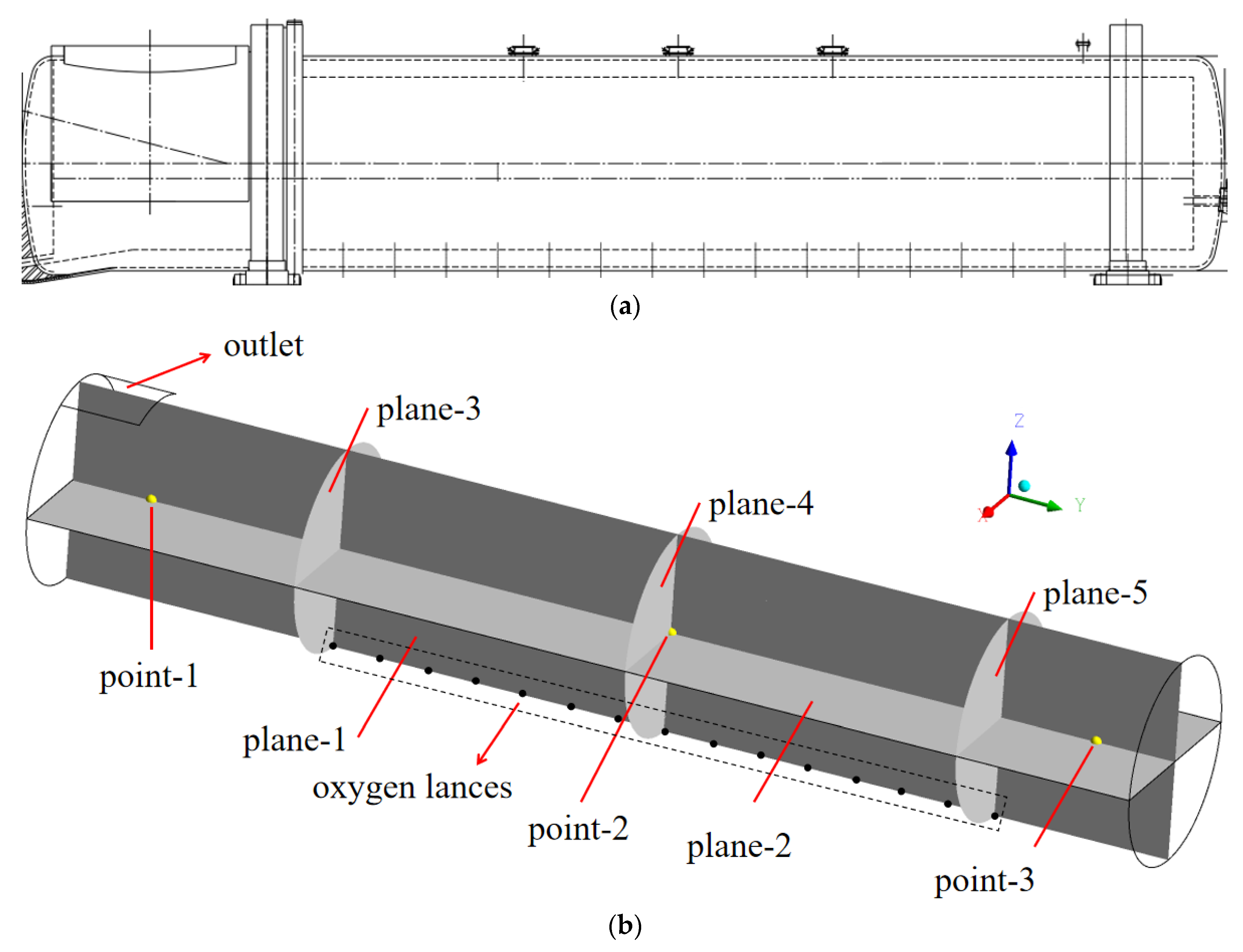
2.1. Geometric Model

Figure 1a shows the actual design of a smelter; numerical simulation is carried out to analyse the flow in the furnace. Analysis of the flow field in different points, planes and regions in the large bottom-blown furnace is helpful to better grasp the flow characteristics in the furnace. The bottom-blowing furnace structure, monitoring points and plane setting used in this simulation experiment are shown in Figure 1b. Each black dot (inlet) in the black dotted box represents the position of each oxygen lance, and the injection rate per oxygen lance is 258 m/s. Type of inlet boundary was velocity inlet and outlet boundary was outlet-vent. Except for the inlet and outlet, the other boundary conditions are wall. The geometric parameters of the bottom-blown furnace used are shown in

Table 1. Geometric parameters of bottom-blowing furnace.

Parameter	Value
Furnace body diameter D (m)	5
Oxygen lance spacing l (m)	2
Oxygen lance diameter d (mm)	50
Depth of molten pool H (m)	2.5
Length of furnace L (m)	28

. The high lead slag’s main components: PbS, accounting for about 50% (ρ = 6000 kg·m⁻³, μ = 0.6 Pa·s) and air (ρ = 1.26kg·m³, μ = 1.9 × 10⁻⁵ Pa·s), were used as working media for simulation calculation; slag is the primary phase and air is the secondary phase, surface tension coefficient between slag and air is 0.38 (N/m). Reference pressure is 101,325 Pa and operation density is 1.225 kg/m³. The entire furnace is meshed with hexahedron. The total number of furnace grids is about 1.05 million. Because the inlet is located at the junction of gas and liquid phase, accompanied by rapid momentum transmission and great change in velocity, in order to ensure the accuracy of calculation, grid encryption is carried out here. The main reactions in the furnace are as follows:

$$\mathrm{PbS}+\frac{3}{2}{\mathrm{O}}_2=\mathrm{PbO}+{\mathrm{SO}}_2$$

2.2. Mathematical Model

(1)

VOF model [27]

The VOF model relies on the fact that two or more fluids (or phases) do not contain each other. Adding an additional phase to the model introduces a variable, the volume fraction of the phase in the calculation cell. Within each control cell, the volume fractions of all phases sum to one. Equations (1) and (2) are the mass and energy conservation equations of the phase q (gas phase or liquid phase):

$$\frac{\partial }{\partial t}\left({\alpha }_q{\rho }_q\right) + \nabla \cdot \left({\alpha }_q {\rho }_q \overrightarrow{v_q}\right) = 0$$

(1)

$$\frac{\partial }{\partial t}\left({\alpha }_q{\rho }_q\overrightarrow{v_q}\right)+\nabla \cdot \left({\alpha }_q{\rho }_q\overrightarrow{v_q\overrightarrow{v_q}}\right) = -\nabla p + \nabla \cdot \left[\mu \left(\nabla \overrightarrow{v_q}+\nabla \overrightarrow{v_q^T}\right)\right]+{\alpha }_q{\rho }_q\overrightarrow{g} + \overrightarrow{f}$$

(2)

$${\alpha }_q={\alpha }_{g}or{\alpha }_l,{\alpha }_g+{\alpha }_l=1$$

(3)

In Equations (1)–(3), α is the volume fraction, ρ is the density, $\overrightarrow{v}$ is the velocity, p is the pressure shared by gas phase and liquid phase, ${\alpha }_q{\rho }_q\overrightarrow{g}$ is the gravity term and $\overrightarrow{f}$ is an external body force. The subscripts g and l represent the gas phase and liquid phase, respectively.

(2)

Standard k−ε model [27]

The standard k−ε model is the most common turbulence model for fluid flow and has a wide range of applications. Through a large number of calculation results and their comparison with experimental results, it is found that the standard k−ε model is used in the calculation of boundary layer flow, pipe flow, shear flow and three-dimensional boundary layer flow simulations, and the results are in good agreement. The two governing equations of the standard k−ε model are as follows:

$$\frac{\partial }{\partial t}\left({\rho }_{m}k\right) + \nabla \cdot \left({\rho }_m\overrightarrow{v_m}k\right) = \nabla \cdot \left({\alpha }_l\frac{{\mu }_t}{{\sigma }_k}\nabla k\right) + G_k + G_b - {\rho }_m$$

(4)

$$\frac{\partial }{\partial t}\left({\rho }_m\epsilon \right) + \nabla \cdot \left({\rho }_m\overrightarrow{v_m}\epsilon \right) = \nabla \cdot \left(\frac{{\mu }_t}{{\sigma }_k}\nabla \epsilon \right) + \frac{\epsilon }{k}\left(C_1\left(G_k+G_b\right)\right)-C_2{\rho }_m\epsilon$$

(5)

In Equations (4) and (5), $G_b$ is the generation of turbulence energy because of buoyancy, $G_k$ is the generation of turbulence energy because of the mean velocity gradients. The definition of mixture density ${\rho }_{\mathrm{m}}$ and mixture velocity $\overrightarrow{v_{\mathrm{m}}}$ are as follows:

$${\rho }_m = {\alpha }_g{\rho }_g + {\alpha }_l{\rho }_l$$

(6)

$$\overrightarrow{v_m} = \frac{{\alpha }_g{\rho }_g\overrightarrow{v_g} + {\alpha }_l{\rho }_l\overrightarrow{v_l}}{{\alpha }_g{\rho }_g + {\alpha }_l{\rho }_l}$$

(7)

where ${\mu }_t$ is the turbulent viscosity:

$${\mu }_t=\rho C_{\mu }\frac{k^2}{\epsilon }$$

(8)

Empirical constants: $C_1=1.44$; $C_2=1.92$; $C_{\mu }=0.09$; ${\sigma }_k=1.0$; ${\sigma }_{\epsilon }=1.3$.

Because the actual bottom-blown furnace structure is complex, it is simplified and modelled. After completing the model establishment and grid division, the mathematical model adopted is as shown in

Table 2. Mathematical model setup.

Model	Method
Multiphase flow model	VOF model
Turbulence model	Standard k-ε model
Wall function	Standard wall function
Discrete scheme of governing equation	Second order upwind scheme
Surface tension	Continuum Surface Force
Pressure discretisation	PRESTO scheme

above, and FLUENT is introduced for unsteady calculation, the time-step was set as 1 × 10⁻³ s, period of process was 5 s, and the convergence condition of each monitoring parameter is that the residual error reaches 1 × 10⁻⁵. After the flow field is stabilised, the experimental data are processed by CFD-POST (ANSYS, Pittsburgh, PA, USA), and important parameters such as flow field characteristics in the furnace are obtained. To simplify the calculation, the model assumes:

(1)

Without considering the chemical reaction, the melt temperature in the initial molten pool is uniformly distributed, and the influence of temperature is ignored.

(2)

The initial height H of static melt in the prototype furnace is half of the furnace diameter D; there is only one phase, high-lead slag, in the molten pool; and the oxygen lance is simplified as a cylinder.

(3)

The gas–liquid interface is treated as a free liquid surface, and the solid wall is regarded as a slip-free boundary, and no wall adhesion.

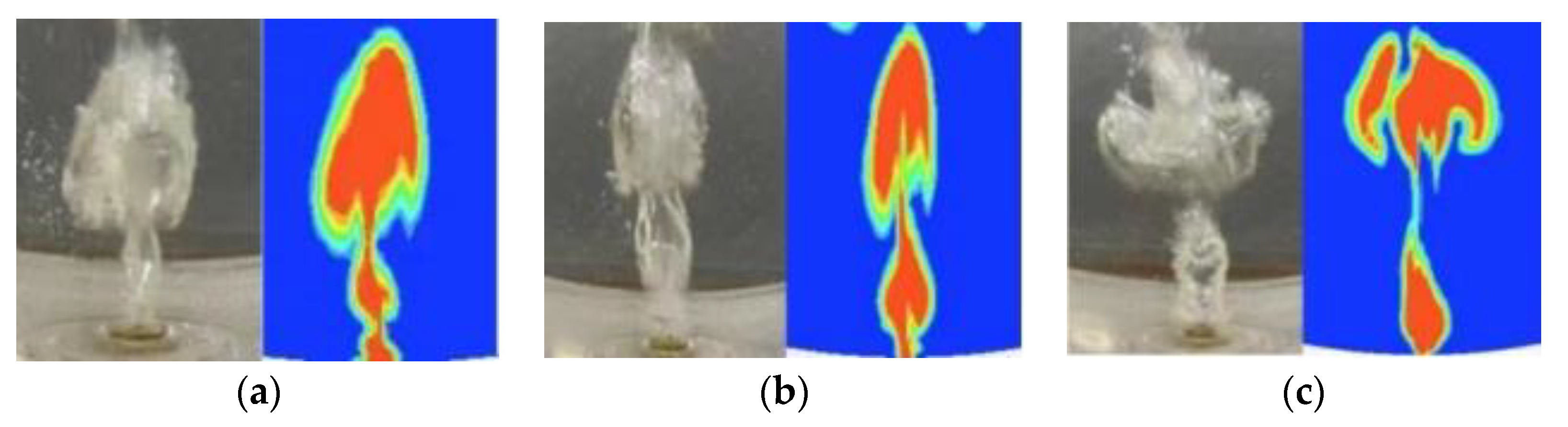
2.3. Validation of Mathematical Model

The verification of the bubble shape at the oxygen lance nozzle is an important evaluation criterion for the establishment of the mathematical model. Limited by the current test conditions, it is not possible to monitor the fluid in the furnace in real time at this stage, so the reliability of the mathematical model cannot be verified by field tests. According to the equal principle of the modified Froude number [11], the results of the numerical simulation of the bubble shape are compared with the actual results of the water model experiment, as shown in Figure 2. Among them, the jet velocity is 30 m/s, the oxygen lance diameter is 5 mm and the liquid level height in furnace is 300 mm. Because the bubble formation at the nozzle of the oxygen lance is a relatively complex process, the calculation instability of the model near the wall area is high. It can be seen that the bubbles at the nozzle of the oxygen lance are approximately ellipsoidal. The bubbles are generated from the bottom in Figure 2a at 1.25 s, gradually grow and become large bubbles in Figure 2b at 1.3 s. When the size reaches a certain level, they begin to break and form small bubbles with irregular shapes in Figure 2c at 1.35 s. After comparison and verification, the numerical simulation results are basically consistent with the experimental observation results, and the matching degree is high.

3. Results and Discussion

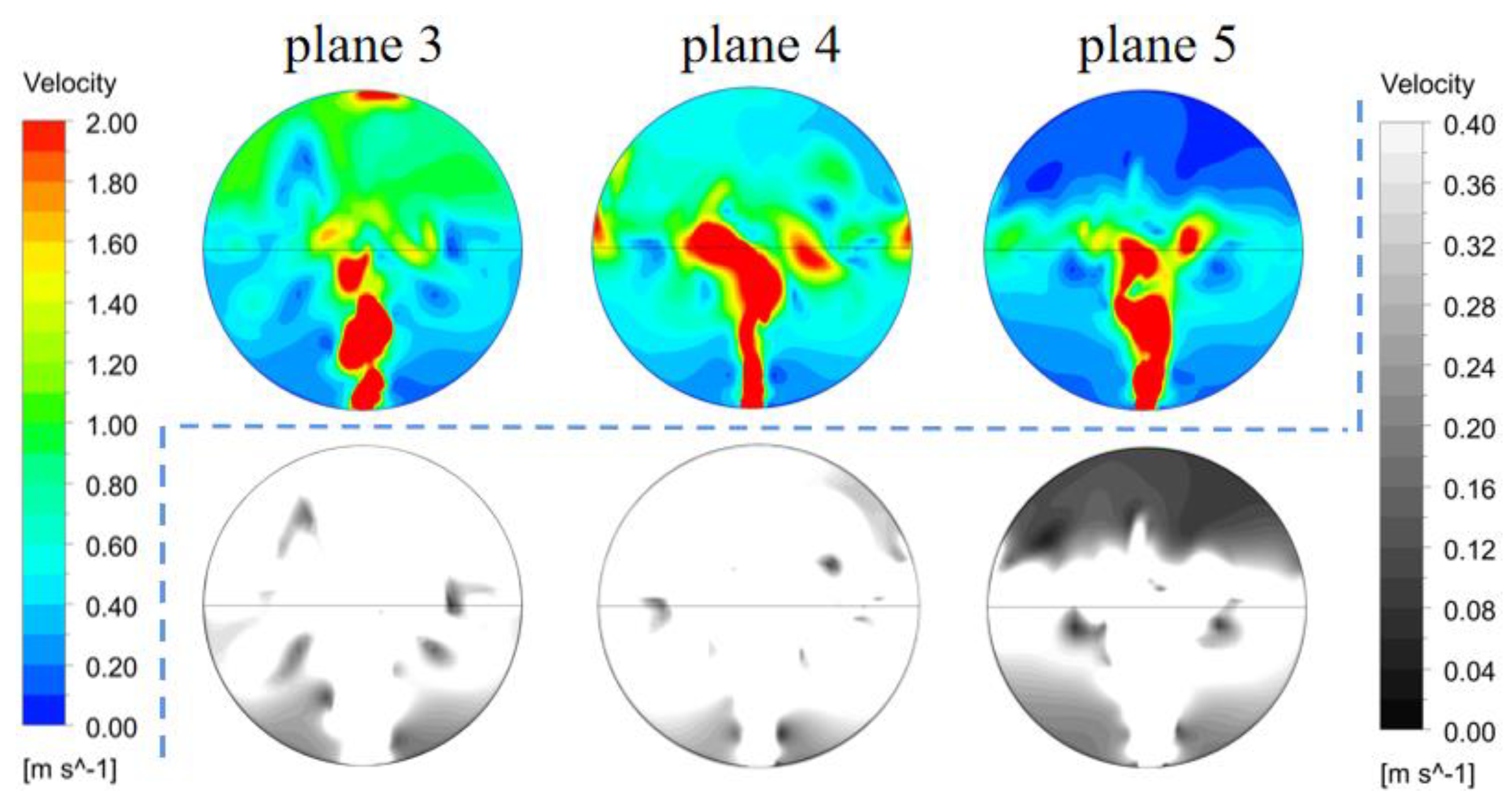
3.1. Plane Flow Field Analysis

Figure 3 shows the velocity distribution and bubble distribution in Plane 1 of a bottom-blown furnace. By analysing Figure 3a,b, it can be seen that the high-velocity region is mainly distributed in the bubble molten pool reaction region (I) at the oxygen lance and the flue gas outlet region (III). The low-velocity region is mainly distributed in the sedimentation region (II) near the wall on both sides of the oxygen lance arrangement region, and there is also a small amount of low-velocity region between oxygen lances. The bubble velocity is obviously higher than the melt velocity. The melt in the melting pool is affected by the high-velocity bubbles, and the momentum between them transmits and is driven to move together, which is beneficial to the stirring and mixing effect in the furnace. However, the instantaneous breakage of the high-velocity bubbles on the liquid surface easily causes the melt in the melting furnace to splash, which is not conducive to the safety of the furnace conditions. The velocity of the sedimentation region is relatively small, which is beneficial to the stable accumulation of crude lead in the furnace, thus avoiding oxidation by oxygen. By integrating the low-velocity region in Figure 3c, the percentage of the gray region in the molten pool (below the yellow line) is calculated to be 48.3%, which is close to half of the molten pool.

Figure 4 shows the distribution of the high-velocity region and low-velocity region in planes 3–5. Observing the molten pool below the black line in each plane, the low-velocity region of the middle oxygen lance in Plane 4 is relatively small. Under this oxygen lance spacing, the flow between two adjacent oxygen lances will affect each other; reducing the existence of the low-velocity region; but the number of oxygen lances is large, which can easily cause waste of gas flow. The low-velocity region of Plane 3 and Plane 5 is obvious; because the oxygen lance in this region is located on both sides of the outermost edge, the interaction between oxygen lances is insufficient. In addition, at Plane 5, there are obviously more low-velocity regions in the gas phase above the black line.

As can be seen from Figure 5a, the high-velocity region at the gas–liquid interface (Plane 2) is mainly distributed near the bubble molten pool reaction region (BMRR) in Figure 2a. Generally speaking, the discharging port is located here, which is more conducive to the mixing of raw materials. As shown in Figure 5b, the low-velocity region is located at the outermost ends of Plane 2, and there is almost no low-velocity region in the BMRR. Observing the velocity vector distribution in Figure 5b, the velocity in the BMRR is mainly transmitted to the upper and lower sides, and then hits the wall and moves to the left and right sides, forming a circulating flow on the liquid surface, which will form an effective agitation effect on the raw materials. Moreover, the velocity vector of the sedimentation region is towards the left and right sides, is far away from the wall and there is a certain distance. The velocity gradually decreases in the process of transmission, which cannot cause a greater impact on the wall of the sedimentation region.

Looking at Figure 6, it can be found that the wall shear stress is mainly distributed at the bottom and both side walls of the region (I), and the shear stress in the sedimentation region is small and negligible. From the velocity vector distribution in Figure 5b, it can be seen that because the high-velocity melt is close to the wall, it is easy to impact the wall, which also explains why there is a large wall shear stress on both side walls of the region (I). Therefore, in actual production, the wearing of refractories on the furnace wall by the molten pool mainly occurs in the region (I) of the furnace, where the furnace wall should be reinforced or special corrosion-resistant materials should be used to reduce the impact of erosion on the furnace structure.

At the initial time of numerical simulation, the bottom-blowing furnace is set to a static state with a velocity of 0 m/s. In the short time at the beginning, the bottom-blowing furnace continuously injects high-velocity gas from the oxygen lance region into the molten pool, which stirs the molten pool violently, and then the flow field of the molten pool reaches a stable state. The required time is defined as “pre-stabilization time”. As shown in Figure 7a, the distribution curves of gas holdup (the volume of the gas phase divided by the total volume of the molten pool) and velocity in Plane 2. The trends of gas holdup and velocity in Plane 2 are roughly similar. Both of them start to reach a stable value at about 2s, so the pre-stabilization time is 2 s. After that, the gas holdup is stable in the range of 3–3.5%, and the velocity in Plane 2 is stable in the range of 1.2–1.4 m/s. At the same time, the internal flow field begins to reach a stable state, which is in line with the normal actual production state.

In order to better understand the distribution of velocity with time in each region, it is necessary to set up monitoring points to analyze the change in velocity. As shown in Figure 7b, the velocity of monitoring points 1–3 varies with time. Before 1 s, the velocity gap between the three monitoring points was still small and basically at the same level. However, after 1 s, the velocity of monitoring point 2 increases obviously, far exceeding the velocity values of monitoring points 1 and 3, and is very unstable. Due to rising rapidly, the bubbles burst instantly at the gas–liquid interface, releasing a large amount of energy which is transmitted around and makes the velocity in this region rise sharply. After a short time, there is no subsequent bubble plume to supplement it, and the velocity begins to decline. On the contrary, the velocity values of monitoring points 1 and 3 are at the same level, in the range of 0–0.2 m/s and in a stable state. Because the distance of monitoring point 1 from the BMRR is farther than that of monitoring point 3, and the influence of the molten pool disturbance is less, the velocity of monitoring point 1 is lower than that of monitoring point 3 as a whole. As shown in Figure 7a, although the whole flow field in the furnace has reached a stable state in about 2 s, there is still an unstable state in the local region similar to that at monitoring point 2. Because of the large volume of the bottom-blown furnace, it has a good slow-release effect on this instability, so the large-scale fluctuation in the local region will not have a great impact on the overall flow field in the furnace.

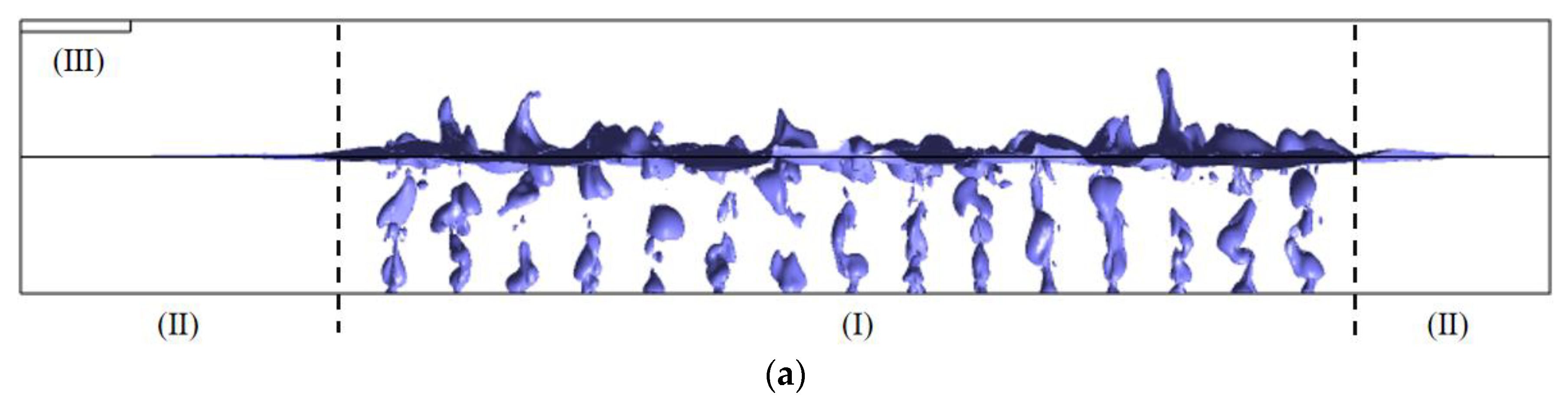
3.2. Analysis of Flow Region in Molten Pool

As shown in Figure 8a, the velocity volume distribution clearly shows the velocity distribution in the furnace. According to Figure 8b,c, the high-velocity region is only distributed in the upper part of the BMRR where the oxygen lance is located, while the low-velocity region is widely distributed in the lower part of the BMRR and the sedimentation region, most of which are located near the wall. Moreover, as can be seen from Figure 8a, the closer to the wall, the smaller the velocity of the molten pool tends to be. The distribution of the dead region (it is less than 0.1 m/s, the fluid is almost at rest, so it is defined as a dead zone) is shown in Figure 8d. The dead region mainly appears in the sedimentation region, and only a few sporadic dead regions exist in the BMRR.

According to the velocity volume distribution in the molten pool, the volume of molten pool in the low-velocity region is captured and calculated as V₁ by data processing software, and the volume of molten pool is determined as V₀. By calculating the percentage of low-velocity region volume in molten pool volume, it is defined as “volume gray scale”, which is represented by symbol E (volume gray scale: the percentage of low-velocity region volume in molten pool volume). Its calculation formula is as follows:

$$\mathrm{E}=\frac{{\mathrm{V}}_1}{{\mathrm{V}}_0}\times 100\%$$

(9)

According to the calculation method of Formula (9), the cumulative percentage of velocity under each velocity is calculated, and the result is shown in

Table 3. Cumulative percentage of velocity.

Velocity/m·s−1	0.2	0.4	0.8	1.6	3.2	6.4	12.8	25.8	51.2
Percentage/%	41.11	66.85	92.07	97.64	99.36	99.86	99.97	99.99	99.999

, which shows that the volume gray scale of this large bottom-blown furnace is 66.85%.

In order to study the nonlinear relationship between cumulative percentage and velocity, it is necessary to establish a suitable mathematical model to predict the cumulative percentage of velocity. Cumulative Distribution Function (CDF), also known as the distribution function, is the integral of the probability density function, which can completely describe the probability distribution of a real random variable X. For all real numbers, the CDF is defined as follows:

$${\mathrm{F}}_{\mathrm{X}}\left(\mathrm{a}\right)=\mathrm{P}\left(\mathrm{X}\le \mathrm{a}\right)$$

(10)

That is, the CDF represents the sum of the occurrence probabilities of all values less than or equal to “a” for independent variable “a”. For this paper, F(a) denotes the probability of the occurrence of velocities less than or equal to “a” in the molten pool region. Obviously, the value of F(a) ranges from 0 to 1, and x ≥ 0. According to the distribution of each point in Table 3, due to the exponential distribution of each point when the velocity value is small (v ≤ 1. 6m/s), it is planned to use an ExponentialCDF mathematical model to fit each point nonlinearly. When x ≥ 0, the formula of the ExponentialCDF mathematical model is:

$$\mathrm{y}={\mathrm{y}}_0+\mathrm{A}\times \left(1-{\mathrm{e}}^{-\mathrm{x}/\mathrm{m}}\right)$$

(11)

According to the data in Table 3, it is easy to know that y₀ = 0 and A = 100. Since y₀ and A are both set values in advance, the only undetermined value is “m”, and the final fitting result is shown in Figure 9. According to the fitting results, it can be found that the fitting effect of the velocity cumulative percentage curve and each point is very good and basically consistent, and the adjusted R square is 0.99851, which indicates that the nonlinear correlation between independent variables and dependent variables is very high, exceeding 99%. The final fitting formula (this formula applies only to this article) of the velocity cumulative percentage is:

$$\mathrm{y}=100\times \left(1-{\mathrm{e}}^{-\frac{\mathrm{x}}{0.37168}}\right) \left(\mathrm{x}\ge 0\right)$$

(12)

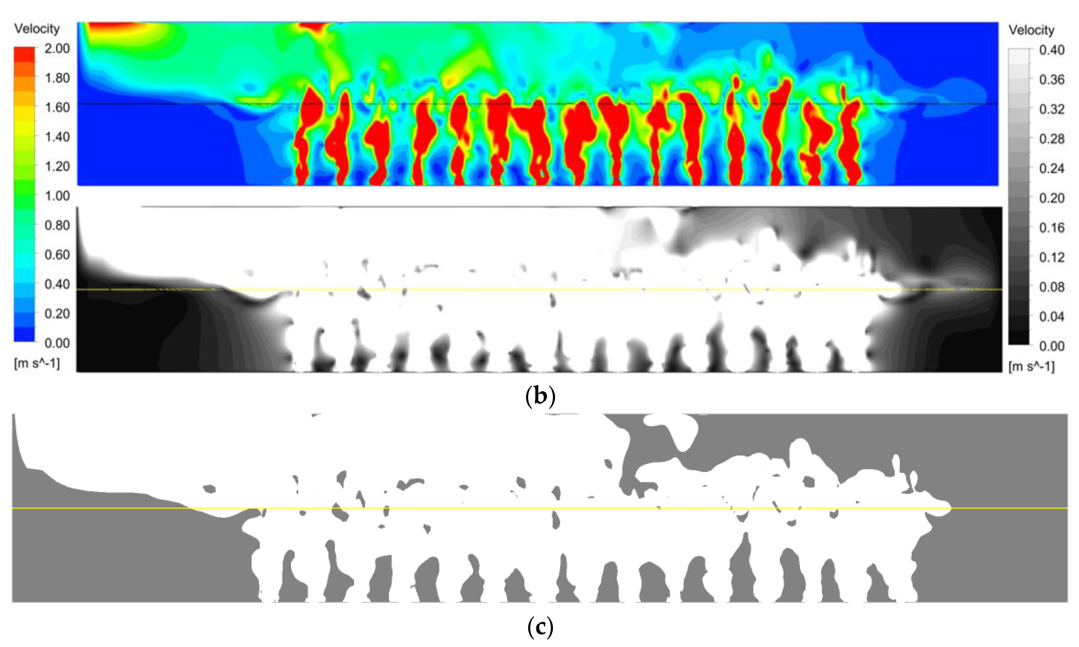
3.3. Bubble Plume in Molten Pool

The bubble plume is divided into three parts: turbulent jet stage or establishment stage; buoyancy plume stage or forming stage; and free surface interaction stage or surface influence stage [30]. As shown in Figure 10a, the bubble plume is mainly distributed in the included angle where the red dotted line is located, and the upper part of the bubble plume is the region where splash concentration exists. With the rise of the bubble plume, the width of the plume is gradually enlarged, it can be found that the bubble plume is not widely distributed in the bottom-blowing furnace molten pool, and there are almost no bubbles on both sides of the bubble plume. To show the relationship between the distribution of the two images, images (a) and (b) are overlapped with 50% transparency. The overlapping image is shown in Figure 10c. Observing Figure 10c shows that the distribution of the bubble plume and the high-velocity region is highly overlapped under the free liquid surface, and the boundary of the high-velocity region basically coincides with the red dotted line in Figure 10a.

4. Conclusions

(1)

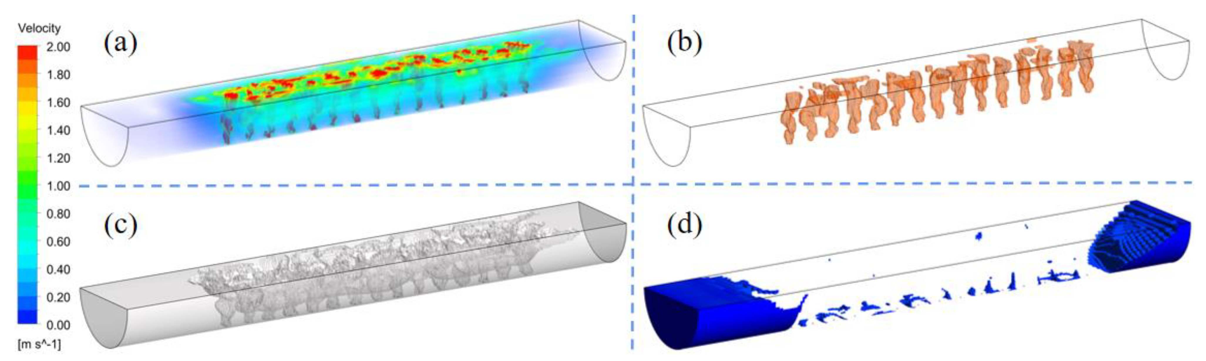
The high-velocity region is mainly distributed in the bubble molten pool reaction region and flue gas outlet region, while the low-velocity region is mainly distributed in the sedimentation region. The flow between two adjacent oxygen lances will influence each other, which effectively reduces the scale of the low-velocity region.

(2)

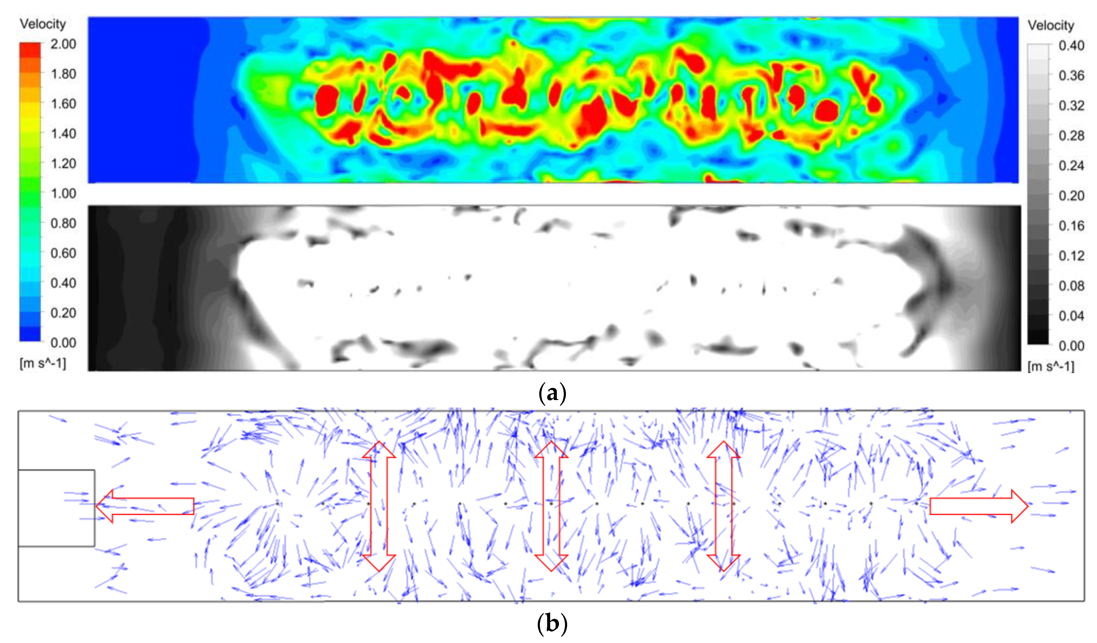
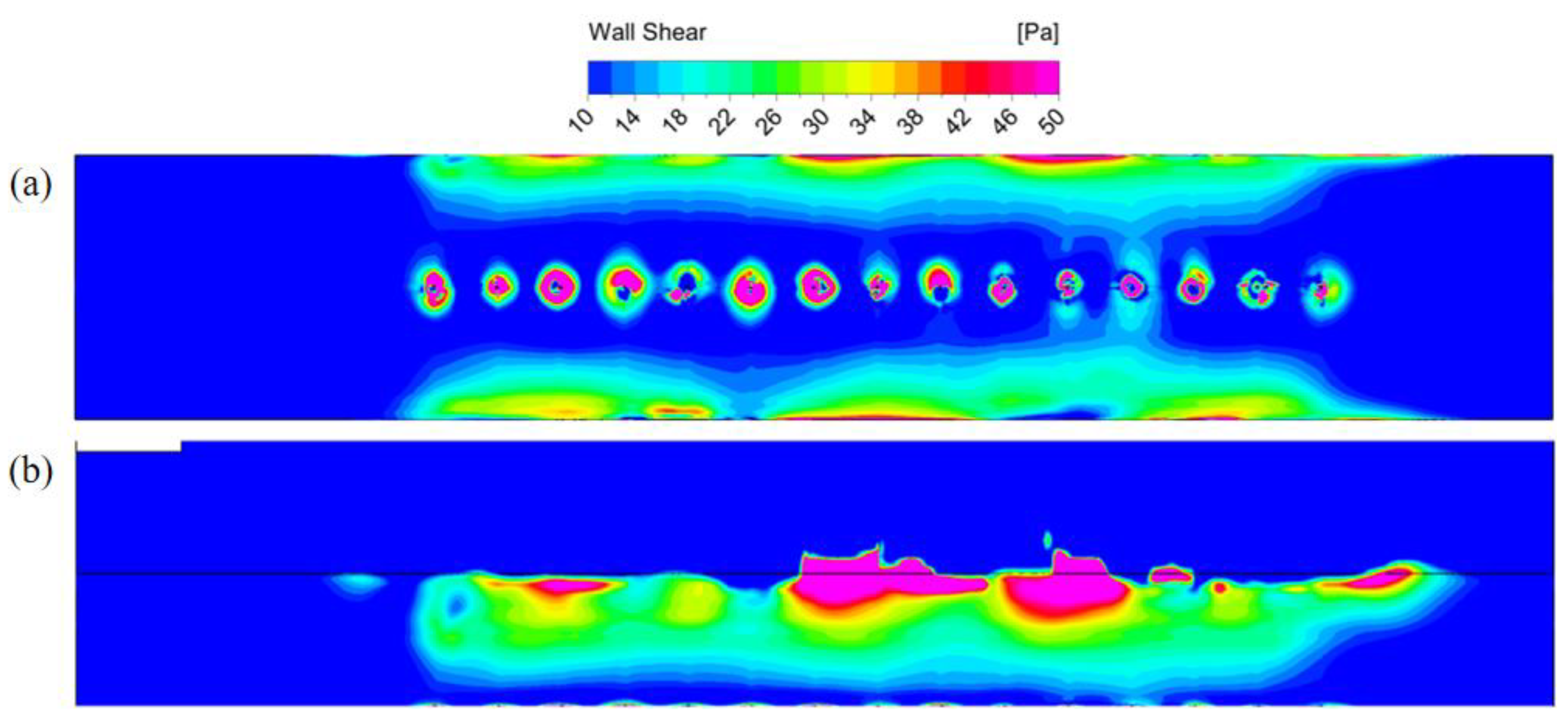
The high-velocity region at the gas–liquid interface is mainly transmitted to the upper and lower sides. Wall shear stress is mainly distributed on the bottom and both sides of the bubble molten pool reaction region.

(3)

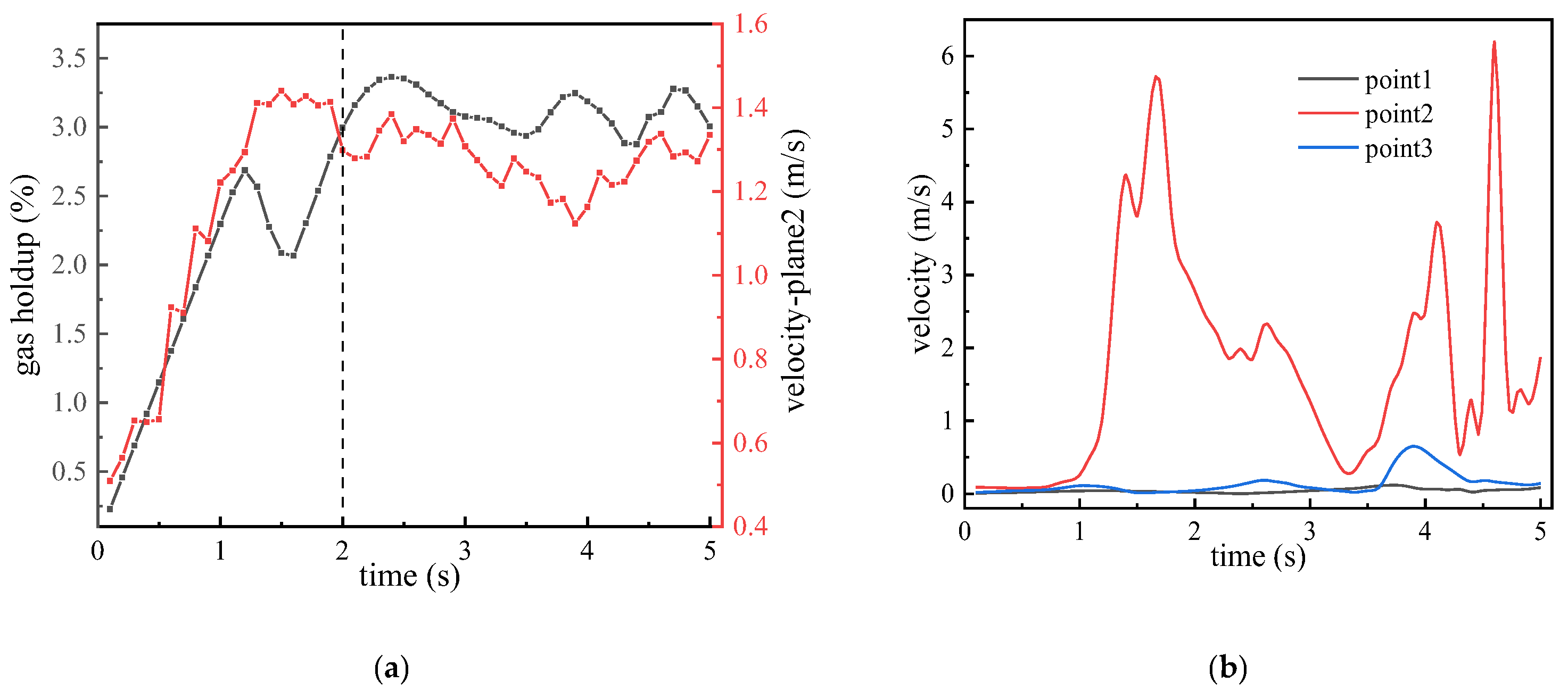
The pre-stabilization time is 2 s. After that, the gas holdup is stable in the range of 3–3.5%, and the velocity in Plane 2 is stable in the range of 1.2–1.4 m/s. The unstable state in the local region will not have a great influence on the overall flow field in the furnace.

(4)

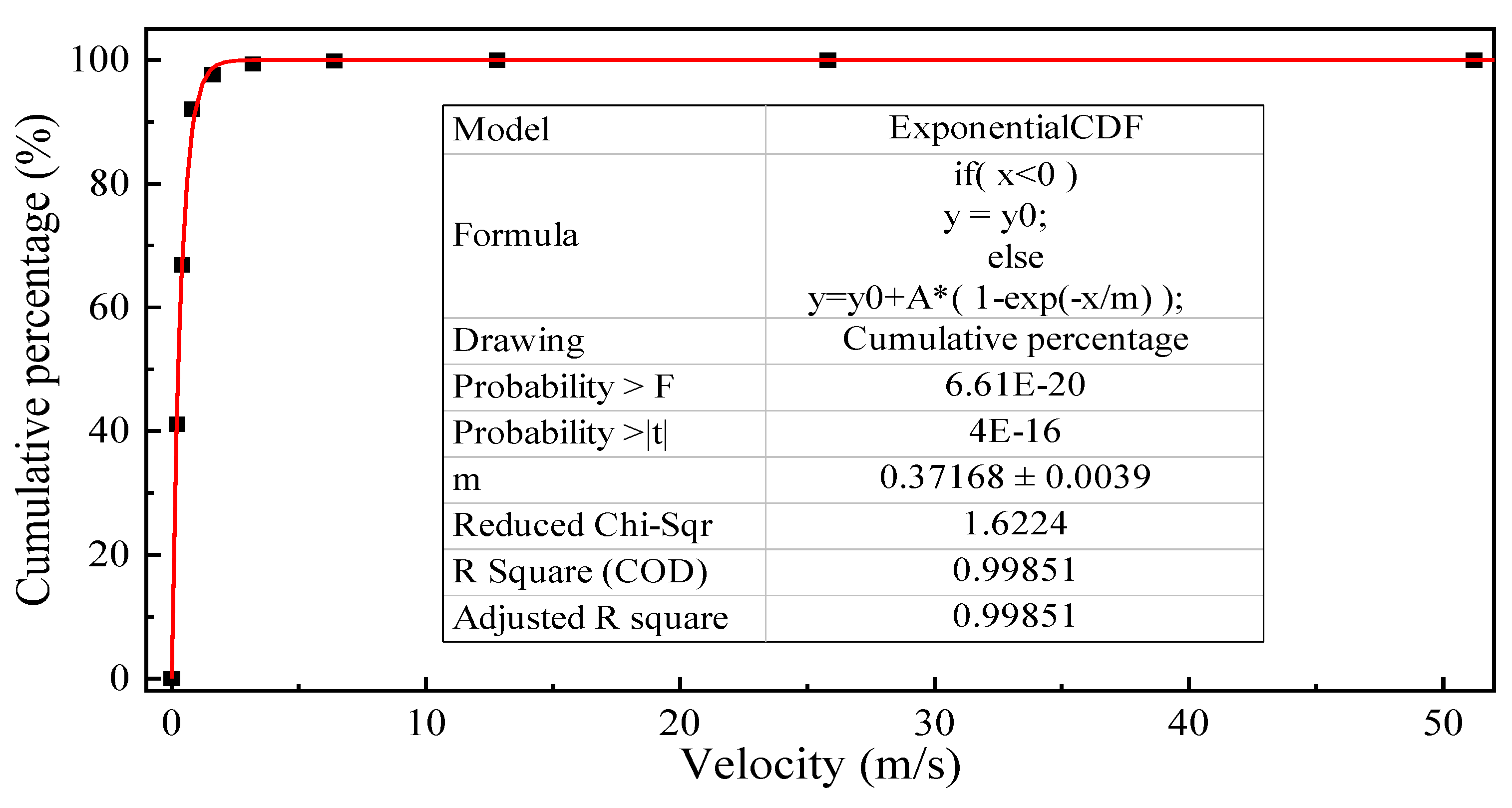
The fitting effect of the velocity cumulative percentage curve and each point is very good and basically coincide with each other.

(5)

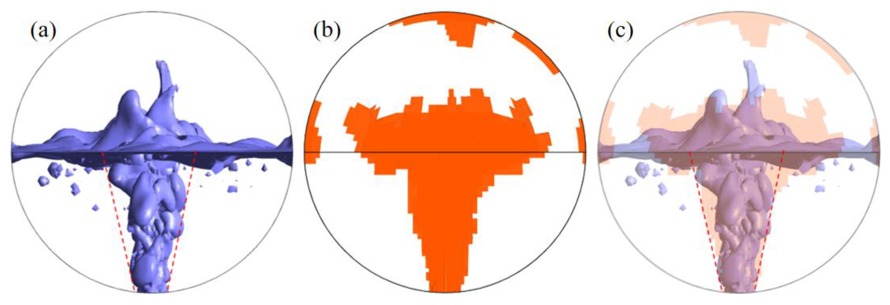
The distribution of the bubble plume and the high-velocity region are highly overlapped under the free liquid surface, and the boundaries of the two regions are basically consistent.

References

1. Zhao, B.; Liao, J. Development of Bottom-Blowing Copper Smelting Technology: A Review. Metals 2022, 12, 190. [Google Scholar] [CrossRef]
2. Bai, L.; Xie, M.; Zhang, Y.; Qiao, Q. Pollution prevention and control measures for the bottom blowing furnace of a lead-smelting process, based on a mathematical model and simulation. J. Clean Prod. 2017, 159, 432–445. [Google Scholar] [CrossRef]
3. Shui, L.; Cui, Z.; Ma, X.; Rhamdhani, M.A.; Nguyen, A.; Zhao, B. Mixing Phenomena in a Bottom Blown Copper Smelter: A Water Model Study. Metall. Mater. Trans. B 2015, 46, 1218–1225. [Google Scholar] [CrossRef]
4. Bumrungthaichaichan, E.; Wattananusorn, S. CFD modelling of pump-around jet mixing tanks: A reliable model for overall mixing time prediction. J. Chin. Inst. Eng. 2019, 42, 428–437. [Google Scholar] [CrossRef]
5. Jiang, X.; Cui, Z.; Chen, M.; Zhao, B. Mixing Behaviors in the Horizontal Bath Smelting Furnaces. Metall. Mater. Trans. B 2019, 50, 173–180. [Google Scholar] [CrossRef]
6. Shao, P.; Jiang, L. Flow and Mixing Behavior in a New Bottom Blown Copper Smelting Furnace. Int. J. Mol. Sci. 2019, 20, 5757. [Google Scholar] [CrossRef] [Green Version]
7. Liu, F.; Zhu, R.; Dong, K.; Bao, X.; Fan, S. Simulation and Application of Bottom-Blowing in Electrical Arc Furnace Steelmaking Process. ISIJ Int. 2015, 55, 2365–2373. [Google Scholar] [CrossRef] [Green Version]
8. Shui, L.; Cui, Z.; Ma, X.; Rhamdhani, M.A.; Nguyen, A.V.; Zhao, B. Understanding of Bath Surface Wave in Bottom Blown Copper Smelting Furnace. Metall. Mater. Trans. B 2016, 47, 135–144. [Google Scholar] [CrossRef]
9. Wei, G.; Zhu, R.; Dong, K.; Ma, G.; Cheng, T. Research and Analysis on the Physical and Chemical Properties of Molten Bath with Bottom-Blowing in EAF Steelmaking Process. Metall. Mater. Trans. B 2016, 47, 3066–3079. [Google Scholar] [CrossRef]
10. Liu, Y.; Yang, T.; Chen, Z.; Zhu, Z.; Zhang, L.; Huang, Q. Experiment and numerical simulation of two-phase flow in oxygen enriched side-blown furnace. Trans. Nonferrous Met. Soc. China 2020, 30, 249–258. [Google Scholar] [CrossRef]
11. Shui, L.; Cui, Z.X.; Ma, X.D.; Jiang, X.; Chen, M.; Xiang, Y.; Zhao, B. A Water Model Study on Mixing Behavior of the Two-Layered Bath in Bottom Blown Copper Smelting Furnace. Jom-Us 2018, 70, 2065–2070. [Google Scholar] [CrossRef]
12. Shui, L.; Ma, X.; Cui, Z.; Zhao, B. An Investigation of the Behavior of the Surficial Longitudinal Wave in a Bottom-Blown Copper Smelting Furnace. Jom-Us 2018, 70, 2119–2127. [Google Scholar] [CrossRef]
13. Wei, G.; Zhu, R.; Wang, Y.; Dong, K.; Wu, X.; Liu, R.; Chen, F. Simulation and application of pulsating bottom-blowing in EAF steelmaking. Ironmak. Steelmak. 2018, 45, 847–856. [Google Scholar] [CrossRef]
14. Song, J.; Xi, W.; Niu, L. Study on the Activity Model of PbO-ZnO-FeO-Fe2O3-SiO2-CaO Six-Component High-Lead Slag System. Metals 2023, 13, 734. [Google Scholar] [CrossRef]
15. Wang, D.; Liu, Y.; Zhang, Z.; Shao, P.; Zhang, T.A. Dimensional Analysis of Average Diameter of Bubbles for Bottom Blown Oxygen Copper Furnace. Math Probl. Eng. 2016, 2016, 1–8. [Google Scholar] [CrossRef] [Green Version]
16. Wang, B.; Shen, S.; Ruan, Y.; Cheng, S.; Peng, W.; Zhang, J. Simulation of Gas-Liquid Two-Phase Flow in Metallurgical Process. Acta Met. Sin. 2020, 56, 619–632. [Google Scholar]
17. Song, K.; Jokilaakso, A. CFD Modeling of Multiphase Flow in an SKS Furnace with New Tuyere Arrangements. Metall. Mater. Trans. B 2022, 53, 253–272. [Google Scholar] [CrossRef]
18. Obiso, D.; Reuter, M.; Richter, A. CFD Investigation of Rotational Sloshing Waves in a Top-Submerged-Lance Metal Bath. Metall. Mater. Trans. B 2021, 52, 2386–2394. [Google Scholar] [CrossRef]
19. Yan, C.; Li, Y.; Zhai, Y.Y.; Sha, Y.H. Numerical Simulation of the Flow of Gases in a Large-Scale Electroslag Furnace. Adv. Mater. Res. 2011, 287, 970–973. [Google Scholar] [CrossRef]
20. Zhou, X.; Ersson, M.; Zhong, L.; Jonsson, P. Numerical Simulations of the Kinetic Energy Transfer in the Bath of a BOF Converter. Metall. Mater. Trans. B 2016, 47, 434–445. [Google Scholar] [CrossRef]
21. Li, Q.; Guo, S.; Wang, S.; Zou, Z. CFD-DEM Investigation on Pressure Drops of Heterogeneous Alternative-Layer Particle Beds for Low-Carbon Operating Blast Furnaces. Metals 2022, 12, 1507. [Google Scholar] [CrossRef]
22. Yao, C.; Jiang, Z.; Zhu, H.; Pan, T. Characteristics Analysis of Fluid Flow and Heating Rate of a Molten Bath Utilizing a Unified Model in a DC EAF. Metals 2022, 12, 390. [Google Scholar] [CrossRef]
23. Ding, W.; Qi, B.; Chen, H.; Li, Y.; Xiong, Y.; Saxén, H.; Yu, Y. Numerical Simulation of Bubble and Velocity Distribution in a Furnace. Metals 2022, 12, 844. [Google Scholar] [CrossRef]
24. Xiao, Y.; Tian, Y.; Wang, Q.; Li, G. Numerical Investigation of Lime Particle Motion in Steelmaking BOF Process. Jom-Us 2021, 73, 2733–2740. [Google Scholar] [CrossRef]
25. Chuang, H.C.; Kuo, J.H.; Huang, C.C. Multi-phase flow simulations in direct iron ore smelting reduction process. ISIJ Int. 2006, 46, 1158–1164. [Google Scholar] [CrossRef] [Green Version]
26. Hu, H.; Yang, L.; Guo, Y.; Chen, F.; Wang, S.; Zheng, F.; Li, B. Numerical Simulation of Bottom-Blowing Stirring in Different Smelting Stages of Electric Arc Furnace Steelmaking. Metals 2021, 11, 799. [Google Scholar] [CrossRef]
27. Song, K.; Jokilaakso, A. CFD Modeling of Multiphase Flow in an SKS Furnace: The Effect of Tuyere Arrangements. Metall. Mater. Trans. B 2021, 52, 1772–1788. [Google Scholar] [CrossRef]
28. Lou, W.; Zhu, M. Numerical Simulation of Slag-metal Reactions and Desulfurization Efficiency in Gas-stirred Ladles with Different Thermodynamics and Kinetics. ISIJ Int. 2015, 55, 961–969. [Google Scholar] [CrossRef] [Green Version]
29. Xi, W.L.; Niu, L.P.; Song, J.B.; Liu, S.H. Numerical Simulation of Flow Field in Large Bottom-Blown Furnace under Different Scale-Up Criteria. Jom-Us 2023, 75, 437–447. [Google Scholar] [CrossRef]
30. Einarsrud, K.E.; Brevik, I. Kinetic Energy Approach to Dissolving Axisymmetric Multiphase Plumes. J. Hydraul. Eng. Asce 2009, 135, 1041–1051. [Google Scholar] [CrossRef] [Green Version]
Figure 1. (a) Structural schematic diagram of large bottom-blowing furnace (b) Tuyere position (0, 6.8–23.6, −2.5) interval 1.2m in Y direction and inclination (90°); Plane 1 (x = 0), Plane 2 (z = 0), Plane 3 (y = 6. 8), Plane 4 (y = 15. 2), Plane 5 (y = 23. 6); Monitoring Point 1 (0, 2, 0), Monitoring Point 2 (0, 15.2, 0) Monitoring Point 3 (0, 26, 0); Unit: m.
Metals 13 01131 g001
Figure 2. Comparison of bubble patterns: (a) Bubble generation; (b) Bubble growth; (c) Bubble break.
Metals 13 01131 g002
Figure 3. Plane 1: (a) Regional distribution; (b) High-velocity region (v ≥ 2 m/s) and low-velocity region (v ≤ 0.4 m/s) distribution; (c) Integrated low-velocity region distribution at 5 s.
Metals 13 01131 g003aMetals 13 01131 g003b
Figure 4. Distribution of high-velocity region and low-velocity region in planes 3–5 at 5 s.
Metals 13 01131 g004
Figure 5. Plane 2: (a) Distribution of high-velocity region and low-velocity region; (b) Velocity vector distribution at 5 s.
Metals 13 01131 g005
Figure 6. Wall shear stress distribution: (a) Bottom view; (b) Side view at 5 s.
Metals 13 01131 g006
Figure 7. (a) Gas holdup and velocity of Plane 2 varies with time; (b) Velocity of monitoring points 1–3 varies with time.
Metals 13 01131 g007
Figure 8. Molten pool: (a) Velocity volume distribution; (b) Volume distribution in high-velocity region, v ≥ 2 m/s; (c) Volume distribution in low-velocity region, v ≤ 0. 4m/s; (d) Volume distribution in dead region, v < 0.1 m/s at 5 s.
Metals 13 01131 g008
Figure 9. Velocity cumulative percentage fitting curve.
Metals 13 01131 g009
Figure 10. Front view of bottom-blown furnace: (a) Bubble plume distribution; (b) High-velocity region distribution; (c) Overlap of bubble plume and high-velocity region at 5 s.
Metals 13 01131 g010