Differential Analysis and Prediction of Planar Shape at the Head and Tail Ends of Medium-Thickness Plate Rolling

Abstract

This paper aims to improve planar shape prediction accuracy in the rolling process of medium and thick plates. We present a model based on the strip method that addresses limitations in predicting planar shape variations at the head and tail ends of rolled pieces. By analysing the rolling process, we introduce the concept of an imaginary strip longitudinal length difference to represent planar shape characteristics effectively. By analysing the change in metal shape in the rolling deformation zone, the calculation formula for metal volume in the deformation zone is derived. This establishes a relationship between the longitudinal length difference at the rolled piece ends and the metal volume in the deformation zone. The prediction of plane shape difference between the end and the head of medium and medium-thickness plate is realized. The experimental results confirm the feasibility and effectiveness of the proposed method.

1. Introduction

The metallurgical industry is constantly evolving, with a focus on improving efficiency, reducing consumption, and promoting environmental sustainability [1,2]. One crucial aspect of this industry is the production of medium and heavy plates, which heavily rely on planar shape control technology during the rolling process. This technology enables manufacturers to increase product yield, minimize waste, and improve economic benefits [3]. Planar shape control technology involves the use of variable thickness rolling methods during production to reduce irregular shapes in rolled products. The ultimate goal is to achieve a more uniform and rectangular plane [4]. The key to this technology is the development of an accurate predictive model for the planar shape of rolled products [5,6,7].

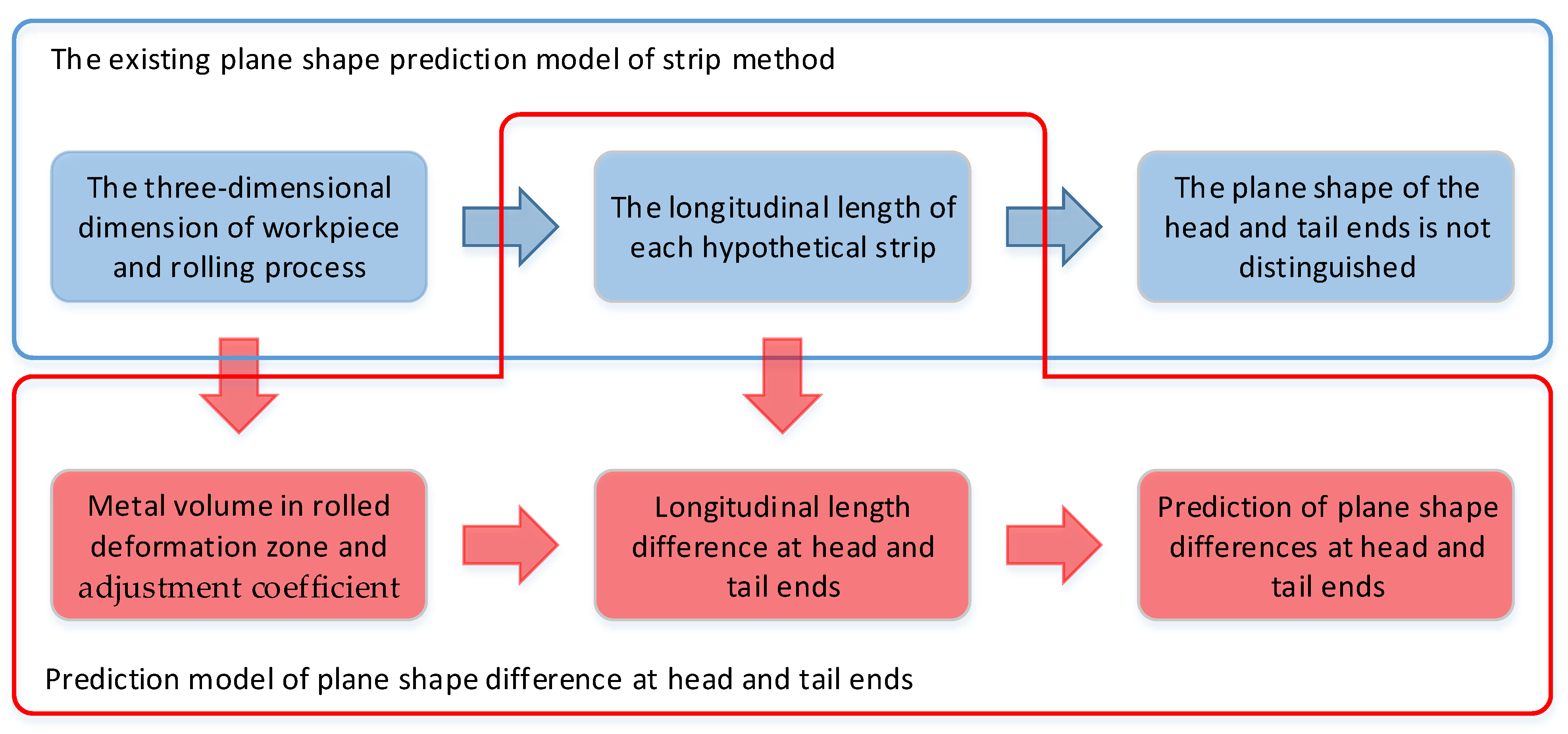
2. Overview of Planar Shape Prediction Models

Scholars worldwide have conducted extensive research on predicting the planar shape of rolled products during the rolling process, leading to significant achievements [8]. For example, a planar shape prediction model has been developed using regression algorithms that determine the functional relationship between rolling parameters and the planar shape of rolled products based on a large volume of experimental data [9,10,11]. Additionally, recent advances in artificial intelligence technology have enabled the use of intelligent techniques in rolling technology development. Intelligent algorithms have been utilized to predict end shapes and width extension data of rolled products, providing further technical means for creating prediction models [12,13,14,15].

Although the prediction accuracy of the aforementioned models meets the demands of practical engineering applications [16], they require a large volume of experimental data for model construction, resulting in high modelling costs [17,18]. Currently, the planar shape prediction models employed in practical engineering are predominantly based on the strip method [2,19]. The core concept involves establishing multiple hypothetical strips along the longitudinal direction of the rolled product [20], as illustrated in Figure 1a. According to the characteristics of metals, during the rolling process, metals undergo three-dimensional deformation. The lateral width extension of metal is greater at the edge of the rolled product than in the middle, while the longitudinal extension is greater in the middle than at the edges [21], as depicted in Figure 1b.

By applying the metal width extension calculation formula, the lateral width extension of each strip can be computed. Assuming that the longitudinal extension of each strip is uniform, based on the principle of constant metal volume and combining the known thickness variations, the longitudinal extension of each strip can be determined [22]. Subsequently, the endpoint positions of each strip can be used to fit an end-plane shape curve, thereby predicting the planar shape of the rolled product’s head and tail ends [23].

3. Analysis of the Differences in Head and Tail End Planar Shape

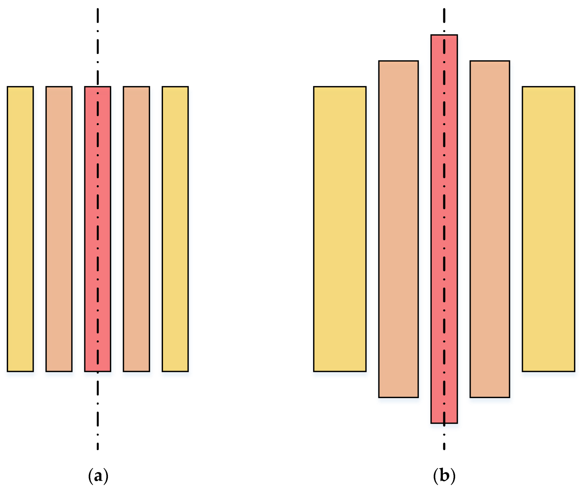
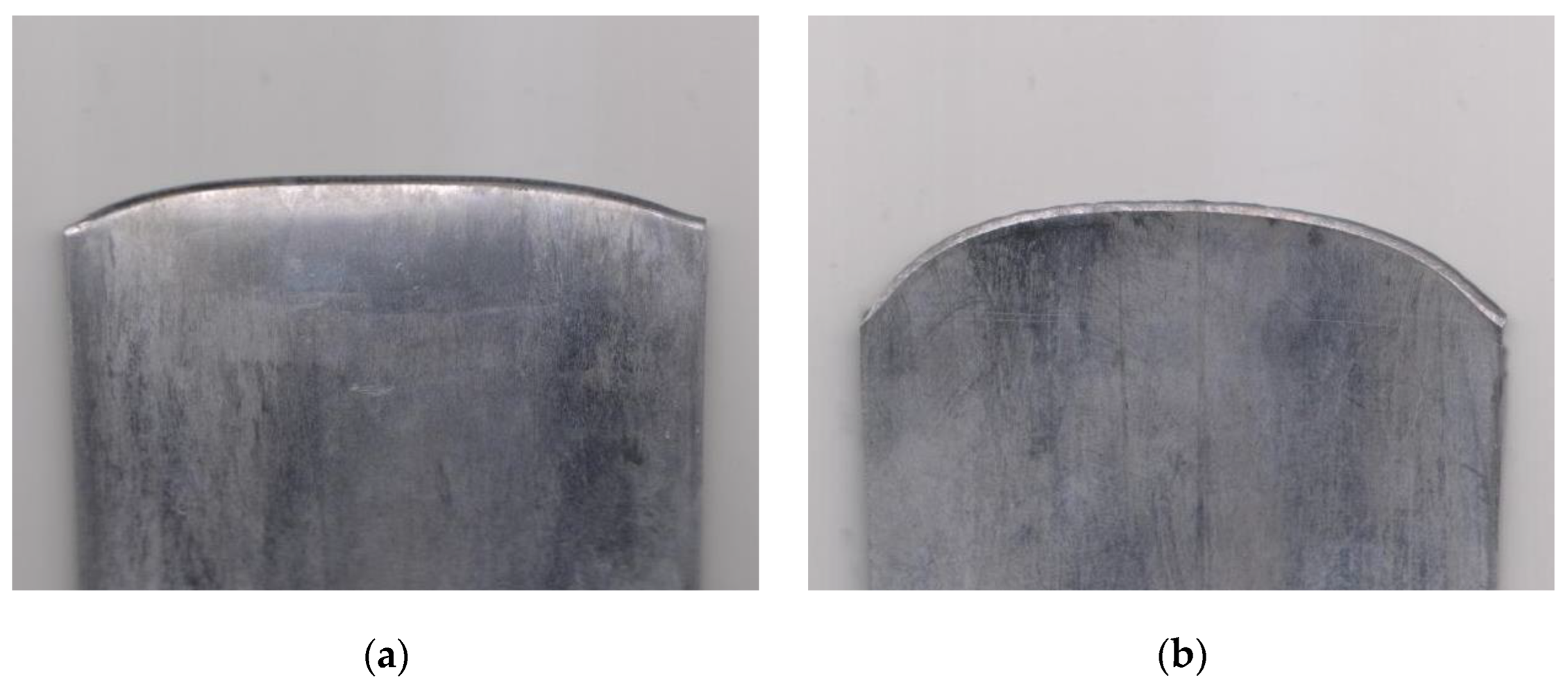
3.1. Differences in Head and Tail End Planar Shape

The key to predicting the planar shape of the head and tail ends of rolled products lies in the calculation of the width extension data for each hypothetical strip, as well as in determining the longitudinal lengths of each strip based on width extensions and thickness variations. Then, by fitting the length of each strip, the shape curves of the head and tail ends of the rolled product can be determined. Existing planar shape prediction models do not differentiate between the shape of the head and tail ends of the rolled product during this process. The calculated results do not consider the distribution ratio of each strip length for the two ends of the rolled product, resulting in identical predictions for the shape of the head and tail ends.

Based on extensive experimental results, the planar shapes of the head and tail ends of rolled products obtained after multiple passes in unidirectional and conventional rolling processes are shown in Figure 2. The curvature of the tail end shape (Figure 2b) is greater than that of the head end shape (Figure 2a), and the irregular shape of the two ends exhibits noticeable differences [24]. There is a certain discrepancy between the existing planar shape prediction models for the head and tail end shapes of rolled products and the actual results [25]. To address such situations, optimization and improvement of the existing planar shape prediction models are required to reflect the differences in the shape of the head and tail ends, satisfying the demands for higher prediction accuracy.

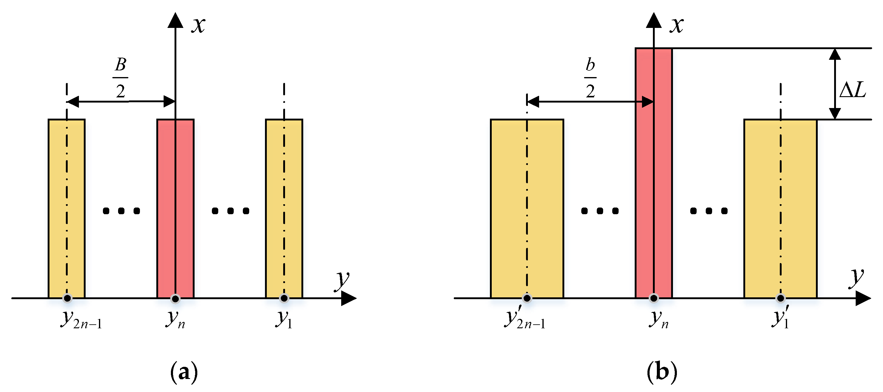
3.2. Determination of End Planar Shape Feature Parameters

According to the strip modelling approach, we hypothetically divide the rolled product into n strips along the longitudinal direction, as shown in Figure 3a. After rolling, the planar shape of the head and tail ends of the rolled product changes, as illustrated in Figure 3b. Based on rolling characteristics, strip n is at the center of the rolled product, with the minimum width extension and maximum longitudinal extension after rolling. Strips 1 and 2n−1 are located at the edges of the rolled product, with the maximum width extension and minimum longitudinal extension after rolling.

The difference between the longitudinal length of any hypothetical strip and the strip edge’s longitudinal length is referred to as the longitudinal length difference of the hypothetical strip. As shown in Figure 3, the longitudinal length difference of each strip can be represented by the sum of the longitudinal length differences of the head and tail ends, with the expression as follows:

$$\left\{\begin{array}{l}{L}_i-L_1=L_i-L_{2n-1}=\Delta L_i\hfill \\ \Delta L_{if}+\Delta L_{ib}=\Delta L_i\hfill \end{array}\right.\begin{array}{cc}& \end{array}\left(2\le i\le 2n-2\right)$$

(1)

where $L_i$ is the longitudinal length of the hypothetical strip i, $\Delta L_i$ is the longitudinal length difference of the hypothetical strip i, $\Delta L_{if}$ is the longitudinal length difference of the head end of the hypothetical strip i, and $\Delta L_{ib}$ is the longitudinal length difference of the tail end of the hypothetical strip i.

Since the longitudinal extension of strip n is the largest, it is referred to as the maximum longitudinal length difference, denoted by $\Delta L$. The head and tail end portions of the maximum longitudinal length difference are called the maximum head-end length difference and the maximum tail-end length difference, denoted by $\Delta L_f$ and $\Delta L_b$, respectively. The distribution ratios of the longitudinal length differences of other hypothetical strips for the head and tail ends can be approximated by the distribution ratios of the maximum longitudinal length difference for the head and tail ends. Based on this, the maximum longitudinal length differences of the head and tail ends can serve as feature parameters to describe the planar shape of the rolled product’s ends, and the ratio of the maximum end length difference to the overall longitudinal length difference can indicate the differences between the head end and tail end of the workpiece.

4. Predicting Differences in Head and Tail End Plane Shapes

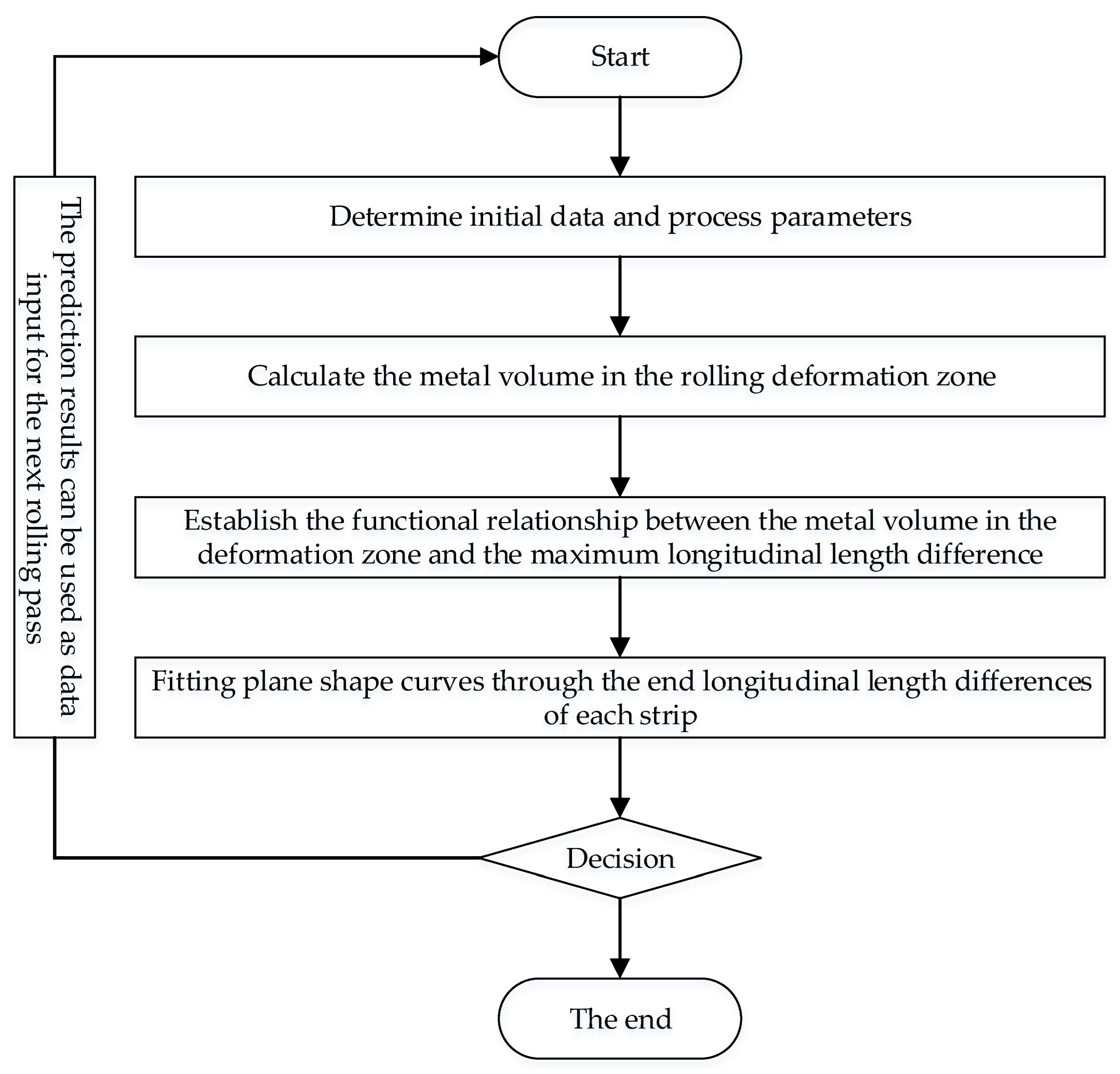
4.1. Modelling Approach for Predicting Differences in Head and Tail End Plane Shapes

The rolling process involves complex three-dimensional deformation of the workpiece between the rolls. The deformation occurs within the rolling deformation zone between the bite section and the rolling outlet section, where the irregular plane shapes of both ends of the workpiece are formed. According to the rolling theory, the rolling deformation zone can be divided into forward slip and backward slip zones. In the forward slip zone, the metal moves in the rolling direction relative to the rotation direction of the rolls, while in the backward slip zone, the metal moves in the opposite direction. The geometric relationship between the rolls and the workpiece indicates that the metal volume in the backward slip zone is larger than that in the forward slip zone, and the deformation amount of the metal in the backward slip zone is greater. Because the deformation of the workpiece follows the principle of volume invariance, the plane shape change of the workpiece is the result of volume change. Therefore, the irregular area of the tail end of the workpiece is larger than that of the head end, which is consistent with the experimental results.

Based on existing plane shape prediction models, a functional relationship between the metal volume in each slip zone within the deformation zone and the maximum longitudinal length difference at the ends representing the plane shape characteristics of the workpiece ends can be established to predict the differences in head and tail end plane shapes. The process is illustrated in Figure 4.

To predict the differences in head and tail end plane shapes, the initial parameters of the workpiece must be determined, including initial dimensions, target dimensions, friction coefficient, neutral angle, reduction rate, rolling pass number, and calculation results of the existing prediction model. Based on these parameters, the metal volume in the rolling deformation zone can be determined. A functional relationship between the metal volume in the deformation zone and the maximum longitudinal length difference at the workpiece ends can be established using a combination of theoretical and experimental approaches. Based on this functional relationship, the longitudinal length differences at the head and tail ends of each strip can be calculated. Fitting plane shape curves through the end longitudinal length differences of each strip allows for predicting the differences in head and tail end plane shapes. The prediction results can be used as data input for the next rolling pass or as the final prediction results.

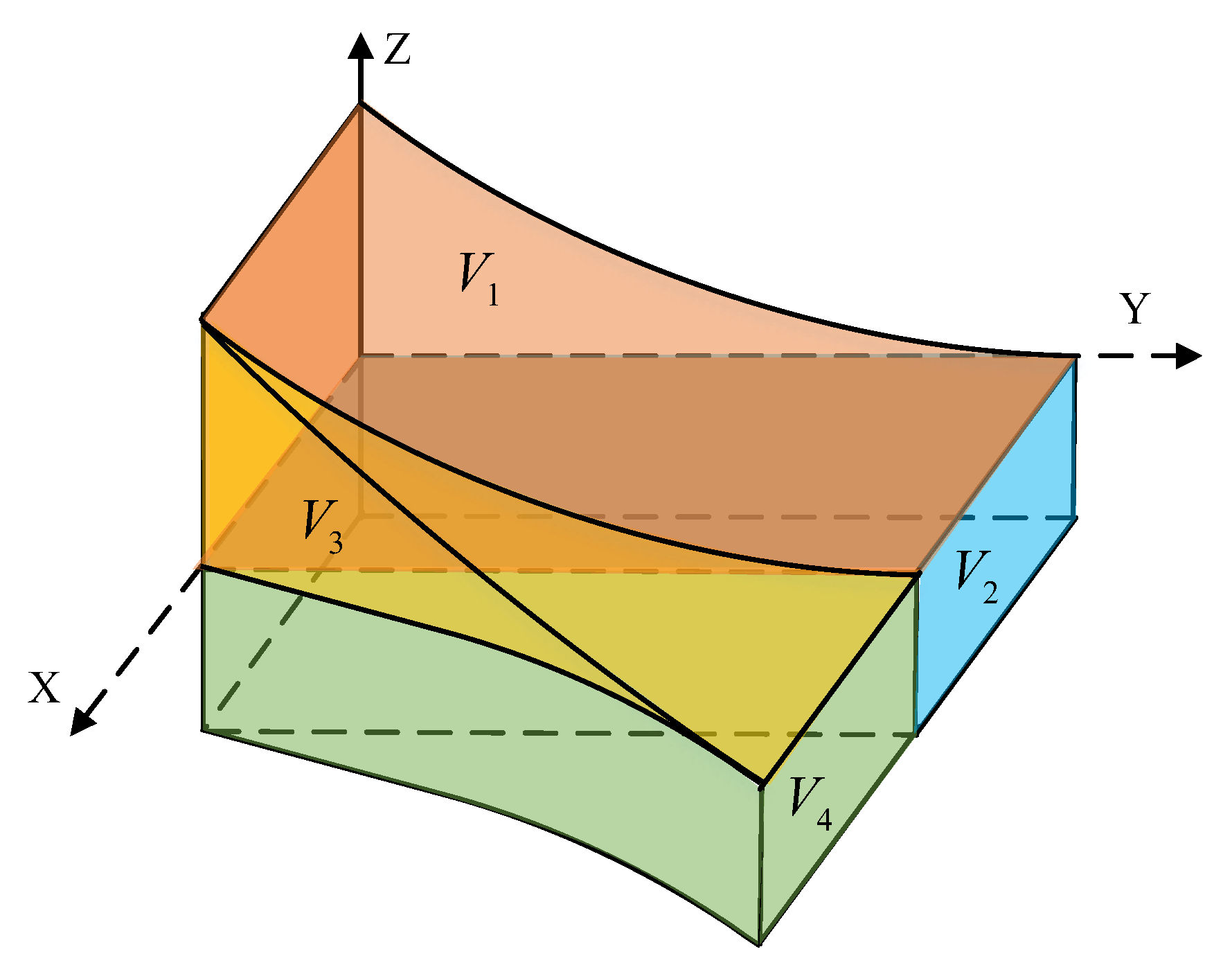
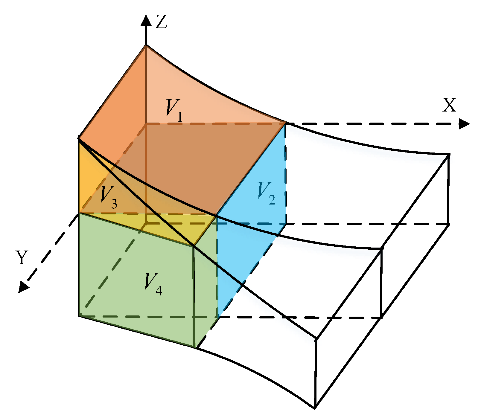
4.2. Calculation of the Workpiece Metal Volume in the Rolling Deformation Zone

For ease of calculation, the workpiece is treated as a steel-plastic body, with one-quarter of the metal in the deformation zone as the research object, and a coordinate system is established. The research object is divided into four parts according to the rolling characteristics and spatial position relationship between the workpiece and the roll gap during the rolling process. In the rolling process, the width change of the workpiece is small compared with the longitudinal change, which leads to the real three-dimensional shape of the workpiece in the rolling deformation zone being difficult to express clearly. Therefore, the metal volume in the rolled deformation zone is properly exaggerated to draw a diagram, as shown in Figure 5. Volume ($V_3$) and ($V_4$) represent the volume of the increased part of the width of the rolled deformation zone.

The volume ($V$) of one-quarter of the metal in the rolling deformation zone can be represented as:

$$V=V_1+V_2+V_3+V_4$$

(2)

The expression for the volume of the first part ($V_1$) of the workpiece metal is:

$$V_1=\frac{1}{2}B{\displaystyle {\int }_0^{l}g(x)dx}$$

(3)

where $l$ is the deformation zone length, $B$ is the width of workpiece before rolling, and ($g(x)$) is the mathematical expression of the contact surface between the roller and the workpiece on the X plane.

Without considering the elastic deformation of the roller, the mathematical expression for a perfect circle ($g(x)$) can be deduced from the geometric relationship between the rolled product and the roller.

$$g(x)=R-\sqrt{R^2-{(x-l)}^2}$$

(4)

where $R$ is the radius of the roller.

By substituting Equation (4) into Equation (3), the expression of $V_1$ is:

$$V_1=\frac{1}{2}B{\displaystyle {\int }_0^l[R-\sqrt{R^2-{(x-l)}^2}]dx}$$

(5)

The volume of the second part ($V_2$) is a rectangular parallelepiped, and it can be represented as:

$$V_2=\frac{1}{4}lBh$$

(6)

where $h$ is the thickness of the workpiece after rolling.

The expression for the volume of the third part ($V_3$) of the rolled product is:

$$V_3={\displaystyle {\int }_0^{l}g(x)f(x)}udx$$

(7)

where $f(x)$ represents the functional expression for the lateral displacement of the rolled product within the deformation zone along the rolling direction, and $u$ represents the lateral displacement of the rolled product on one side of the exit of the deformation zone.

Based on a significant amount of rolling experiments, the edge shape curve of the rolled product has been measured, and $f(x)$ can be expressed as [20]:

$$f(x)=3{(\frac{x}{l})}^2-2{(\frac{x}{l})}^3$$

(8)

By substituting Equations (4) and (8) into Equation (7), the expression for the third part of the metal volume ($V_3$) can be expressed as:

$$V_3={\displaystyle {\int }_0^l[R-\sqrt{R^2-{(x-l)}^2}]}\cdot [3{(\frac{x}{l})}^2-2{(\frac{x}{l})}^3]udx$$

(9)

The expression for the volume of the fourth part of the metal ($V_4$) in the rolled product is:

$$V_4=\frac{1}{2}uh{\displaystyle {\int }_0^{l}f(x)}dx$$

(10)

By substituting Equation (8) into Equation (10), the expression for the volume of the fourth part ($V_4$) can be expressed as:

$$V_4=\frac{1}{2}hu{\displaystyle {\int }_0^l[3{(\frac{x}{l})}^2-2{(\frac{x}{l})}^3]}dx$$

(11)

By substituting Equations (5), (6), (9), and (11) into Equation (2), the formula for calculating the metal volume ($V$) in 1/4 of the rolling deformation zone can be derived as follows:

$$\begin{array}{l}V=\frac{1}{2}B{\displaystyle {\int }_0^l[R-\sqrt{R^2-{(x-l)}^2}]dx}+\frac{1}{4}lBh\\ +{\displaystyle {\int }_0^l[R-\sqrt{R^2-{(x-l)}^2}]}\cdot [3{(\frac{x}{l})}^2-2{(\frac{x}{l})}^3]udx\\ +\frac{1}{2}hu{\displaystyle {\int }_0^l[3{(\frac{x}{l})}^2-2{(\frac{x}{l})}^3]}dx\end{array}$$

(12)

The calculation approach for the volume of the backward slip zone of the rolled product ($V_b$) is consistent with that of the overall deformation zone, and the trailing region volume is divided into four parts, as illustrated in Figure 6.

As shown in the diagram, the spatial position of the trailing region of the rolled product indicates that the expression for the 1/4 metal volume ($V_b$) in the backward slip zone is:

$$V_b=V_{b1}+V_{b2}+V_{b3}+V_{b4}$$

(13)

The expression for the volume of the first part of the metal ($V_{b1}$) in the backward slip zone is:

$$V_{b1}=\frac{1}{2}B{\displaystyle {\int }_0^{l_2}[R-\sqrt{R^2-{(x-l)}^2}]dx}$$

(14)

where $l_2$ is the longitudinal length of the backward slip zone.

The expression for the volume of the second part of the metal ($V_{b2}$) in the backward slip zone is:

$$V_{b2}=\frac{1}{2}B{l}_{2}R(1-\cos \gamma )+\frac{1}{4}B{l}_{2}h$$

(15)

where $\gamma$ is a neutral angle.

The expression for the volume of the third part of the metal ($V_{b3}$) in the backward slip zone is:

$$V_{b3}={\displaystyle {\int }_0^{l_2}[R-\sqrt{R^2-{(x-l)}^2}]}\cdot [3{(\frac{x}{l})}^2-2{(\frac{x}{l})}^3]udx$$

(16)

The expression for the volume of the fourth part of the metal ($V_{b4}$) in the backward slip zone is:

$$V_{b4}=u\left[R(1-\cos \gamma )+\frac{1}{2}h\right]{\displaystyle {\int }_0^l[3{(\frac{x}{l})}^2-2{(\frac{x}{l})}^3]}dx$$

(17)

By substituting Equations (14)–(17) into Equation (13), the formula for calculating the metal volume ($V_b$) in 1/4 of the backward slip zone can be derived as follows:

$$\begin{array}{l}{V}_b=\frac{1}{2}B{\displaystyle {\int }_0^{l_2}[R-\sqrt{R^2-{(x-l)}^2}]dx}+\frac{1}{2}B{l}_{2}R(1-\cos \gamma )\\ +\frac{1}{4}B{l}_{2}h+{\displaystyle {\int }_0^{l_2}[R-\sqrt{R^2-{(x-l)}^2}]}\cdot [3{(\frac{x}{l})}^2-2{(\frac{x}{l})}^3]udx\\ +u\left[R(1-\cos \gamma )+\frac{1}{2}h\right]{\displaystyle {\int }_0^l[3{(\frac{x}{l})}^2-2{(\frac{x}{l})}^3]}dx\end{array}$$

(18)

According to the geometric relationship of the rolling deformation zone, the mathematical expression of the volume of the forward slip zone ($V_f$) is determined as follows:

$$V_f=V-V_b$$

(19)

4.3. Establishing the Prediction Model

The functional relationship between the metal volume in the slip zone and the corresponding maximum longitudinal length difference at the workpiece ends was determined. The important rolling parameters under different numerical conditions were simulated by the finite element modelling method to determine the correlation between these parameters and the difference in end plane shapes. According to the simulation results, although some important rolling parameters are related to the plane shape of the workpiece, they have little effect on the difference in plane shapes at the head and tail ends of the workpiece, such as friction coefficient, workpiece length, and rolling speed. The parameters directly related to the difference in plane shapes at the head and tail ends of the workpiece are the width-to-thickness ratio and reduction rate.

Based on this law, the rolling experiment is carried out, and the experimental results are analysed. The dimensions of the specimens and the characteristics of the rolling process are shown in

Table 1. The dimensions of the specimens and the rolling process.

Number of Workpieces	The Width of Workpieces (mm)	The Thickness of Workpieces (mm)	The Length of Workpieces (mm)	The Characteristics of the Rolling Process
1	30	16	70	Rolling experiments can be conducted on specimens of different dimensions using the same rolling process, rolling 8 passes.
2	50	16	70
3	90	16	70

.

The experimental results are collated, and the maximum longitudinal length differences at the head and tail ends of the workpieces for each rolling pass are calculated. The proportion of the metal volume in the slip zone within the overall deformation zone is compared with the proportion of the corresponding maximum end length difference in the overall length difference, and a line graph is plotted, as shown in Figure 7.

Analysing the graph reveals that after several rolling passes, the proportion of the metal volume in each slip zone within the overall deformation zone converges with the proportion of the corresponding maximum end length difference in the overall length difference. When the width-to-thickness ratio and reduction rate of the workpiece are changed, the two lines remain parallel, but the vertical distance changes. This indicates that there is a functional relationship between the proportion of the maximum longitudinal length differences at the head and tail ends and the proportion of the metal volume in the forward and backward slip zones within the overall deformation zone, as shown:

$$\left\{\begin{array}{c}\frac{\Delta L_f}{\Delta L}=\frac{V_f}{V}+a_f\\ \begin{array}{l}\frac{\Delta L_b}{\Delta L}=\frac{V_b}{V}+a_b\\ a_f=-a_b\end{array}\end{array}\right.$$

(20)

In the above equation, constants $a_f$ and $a_b$ are the adjustment coefficients for the proportions of the metal volume in the overall deformation zone and the maximum longitudinal length differences in the overall length difference, respectively. Based on the experimental results, the constants are affected by the reduction rate and width-to-thickness ratio of the workpiece, and they are opposite in value. $a_f$ is directly proportional to the reduction rate and inversely proportional to the width-to-thickness ratio, while $a_b$ is inversely proportional to the reduction rate and directly proportional to the width-to-thickness ratio.

Using the experimental results as a data basis and applying the least squares method, the functional relationships between the adjustment coefficients and the reduction rate and width-to-thickness ratio can be determined as follows:

$$\left\{\begin{array}{l}{a}_f=-0.02R_H+1.7\epsilon \begin{array}{ccc}& & (R_H\le 10)\end{array}\hfill \\ a_f=-0.015R_H+1.2\epsilon \begin{array}{ccc}& & (R_H>10)\end{array}\hfill \\ a_f=-a_b\hfill \end{array}\right.$$

(21)

where $R_H$ is width-to-thickness ratio of the workpiece, and $\epsilon$ is the reduction rate.

In the existing plane shape prediction model, the first and 2n−1th strips are considered the edges of the workpiece, with a longitudinal length difference of zero. The distribution ratio of the longitudinal length differences at the head and tail ends for the remaining hypothetical strips can be calculated based on the proportions of the maximum longitudinal length differences at the two ends in the overall length difference, as expressed below:

$$\left[\begin{array}{c}\Delta L_{2f}\\ \Delta L_{3f}\\ ·\\ ·\\ ·\\ \Delta L_{(2n-2)f}\end{array}\right]=\left[\begin{array}{c}\Delta L_2\\ \Delta L_3\\ ·\\ ·\\ ·\\ \Delta L_{2n-2}\end{array}\right]\frac{\Delta L_f}{\Delta L}\begin{array}{cc}& \end{array}\begin{array}{cc}& \end{array}\begin{array}{cc}& \end{array}\left[\begin{array}{c}\Delta L_{2b}\\ \Delta L_{3b}\\ ·\\ ·\\ ·\\ \Delta L_{(2n-2)b}\end{array}\right]=\left[\begin{array}{c}\Delta L_2\\ \Delta L_3\\ ·\\ ·\\ ·\\ \Delta L_{2n-2}\end{array}\right]\frac{\Delta L_b}{\Delta L}$$

(22)

Based on the results of Equation (22) and the horizontal expansion of each hypothetical strip calculated using the existing plane shape prediction model, the coordinates of the endpoints at the head and tail ends of each strip can be determined. By fitting the plane shape curves to the endpoint coordinates, the prediction of the differences in head and tail end plane shapes can be realized.

5. Application Conditions and Interpretation of Prediction Model of End Plane Shape Difference

5.1. Application Condition for Prediction Model of End Plane Shape Difference

The purpose of predicting the difference in the plane shape of the workpiece head and tail is to eliminate the defect that the prediction model based on the strip method cannot distinguish the plane shape at the head and tail end of the workpiece. The relationship between the prediction model of end plane shape difference and the existing plane shape prediction model is shown in Figure 8.

As shown in Figure 8, the application conditions for the prediction model of plane shape difference at head and tail ends mainly consist of two parts. The first part is to determine the metal volume of the rolling deformation area and the adjustment factor of the maximum longitudinal length difference at the end according to the workpiece geometry size and process parameters. The second part is the application of the existing plane shape prediction model of the strip method to calculate the longitudinal length of each hypothetical strip.

5.2. Interpretation of Prediction Model of End Plane Shape Difference

In this paper, based on the strip method, it is proposed to use the longitudinal maximum length difference to represent the plane shape of the workpiece end. Similarly, the ratio of the maximum longitudinal length difference at the end to the overall length difference can represent the difference in the plane shape of the head end and the tail end. Because the plane shape change of the workpiece is the result of volume change, the functional relationship between the metal volume in the rolling deformation zone and the maximum length difference at the end can be established to predict the plane shape difference at the head and tail ends of the workpiece.

The prediction model of plane shape difference is divided into two parts. First, the volume of metal in the rolling deformation zone needs to be calculated, which is essentially a geometric problem. The metal volume in the rolling deformation zone is affected by rolling process parameters, such as roll radius, plate width, and the rolling reduction. Equations (2)–(19) in this paper attempt to establish a functional relationship between the rolling process parameters and metal volume in the rolling deformation zone.

Part two is to establish a functional relationship between the metal volume in the deformation zone and the difference in the longitudinal length of the workpiece end. The modelling process involves using the finite element simulation method to determine the macroscopic law and then implement the rolling experiment. Based on the experimental data, the least square method is used to determine the function relation.

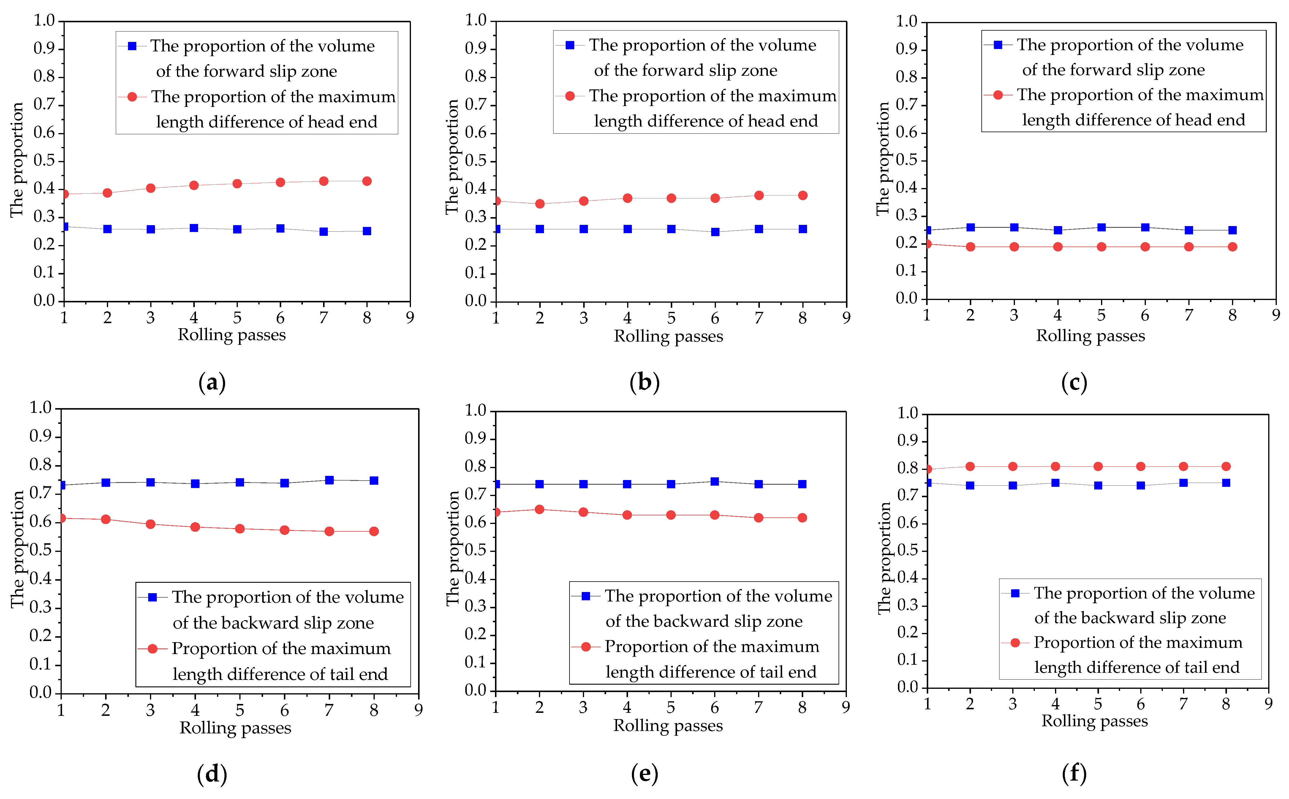
6. Application Effect of the Head and Tail End Plane Shape Difference Prediction Model

In order to verify the correctness of the prediction model of plane shape differences at the head and tail ends, finite element simulation and experimental verification are used.

The same rolling process is used in the finite element simulation and experiment. The rolling process parameters are shown in

Table 2. The table of rolling process parameters.

Rolling Pass	The Thickness of Workpieces (mm)	The Rolling Reduction (mm)	The Rolling Reduction Ratio	The Width-to-Thickness Ratio of Workpieces
1	16.0	0.6	0.038	6.00
2	15.4	0.6	0.039	6.24
3	14.8	0.6	0.041	6.49
4	14.2	0.6	0.042	6.77
5	13.6	0.6	0.044	7.08
6	13.0	0.6	0.046	7.41
7	12.4	0.6	0.048	7.77
8	11.8	0.6	0.051	8.17
9	11.2	0.6	0.054	8.61
10	10.6	0.6	0.057	9.11
11	9.4	1.2	0.128	10.28
12	8.2	1.2	0.146	11.80
13	7.0	1.2	0.171	13.84
14	5.8	1.2	0.207	16.72
15	4.6	1.2	0.261	21.11

.

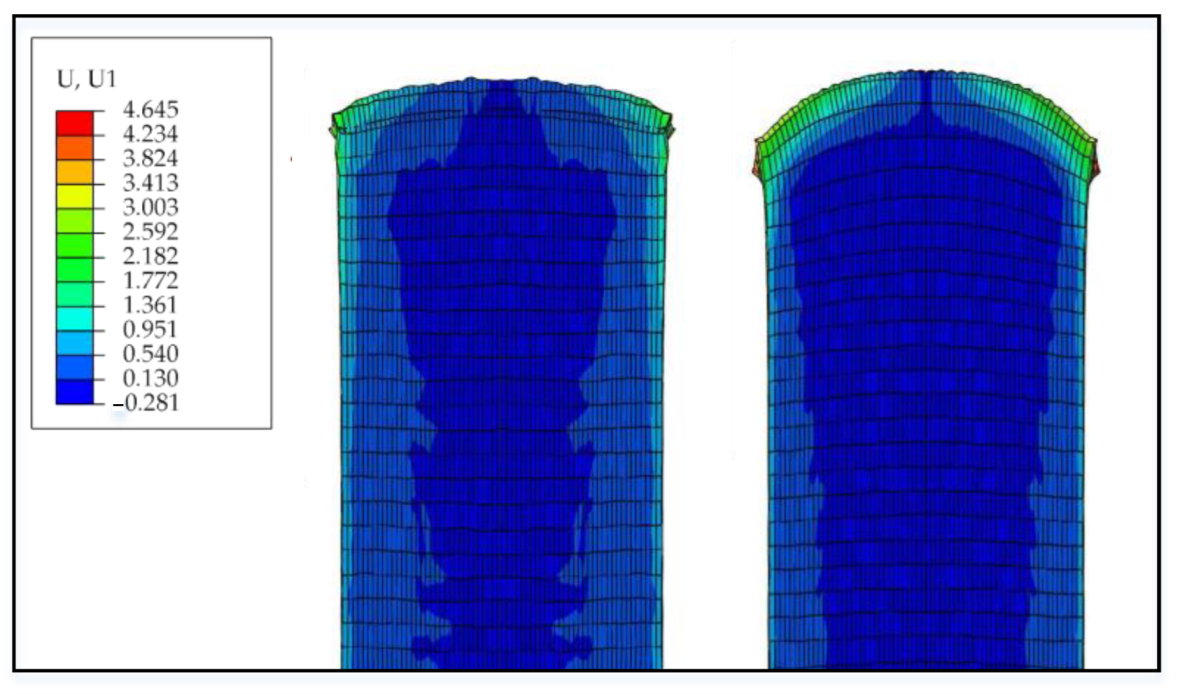
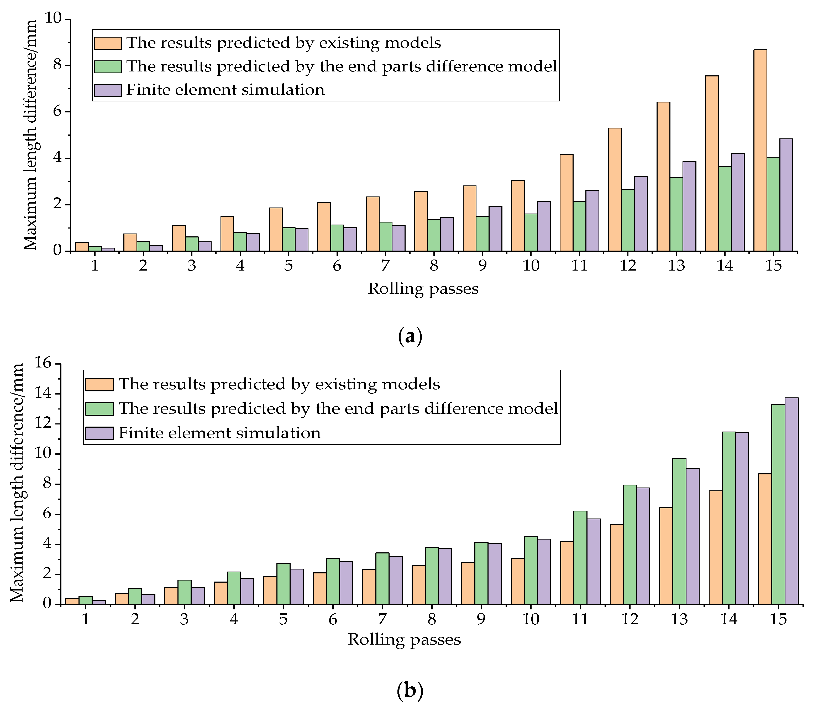
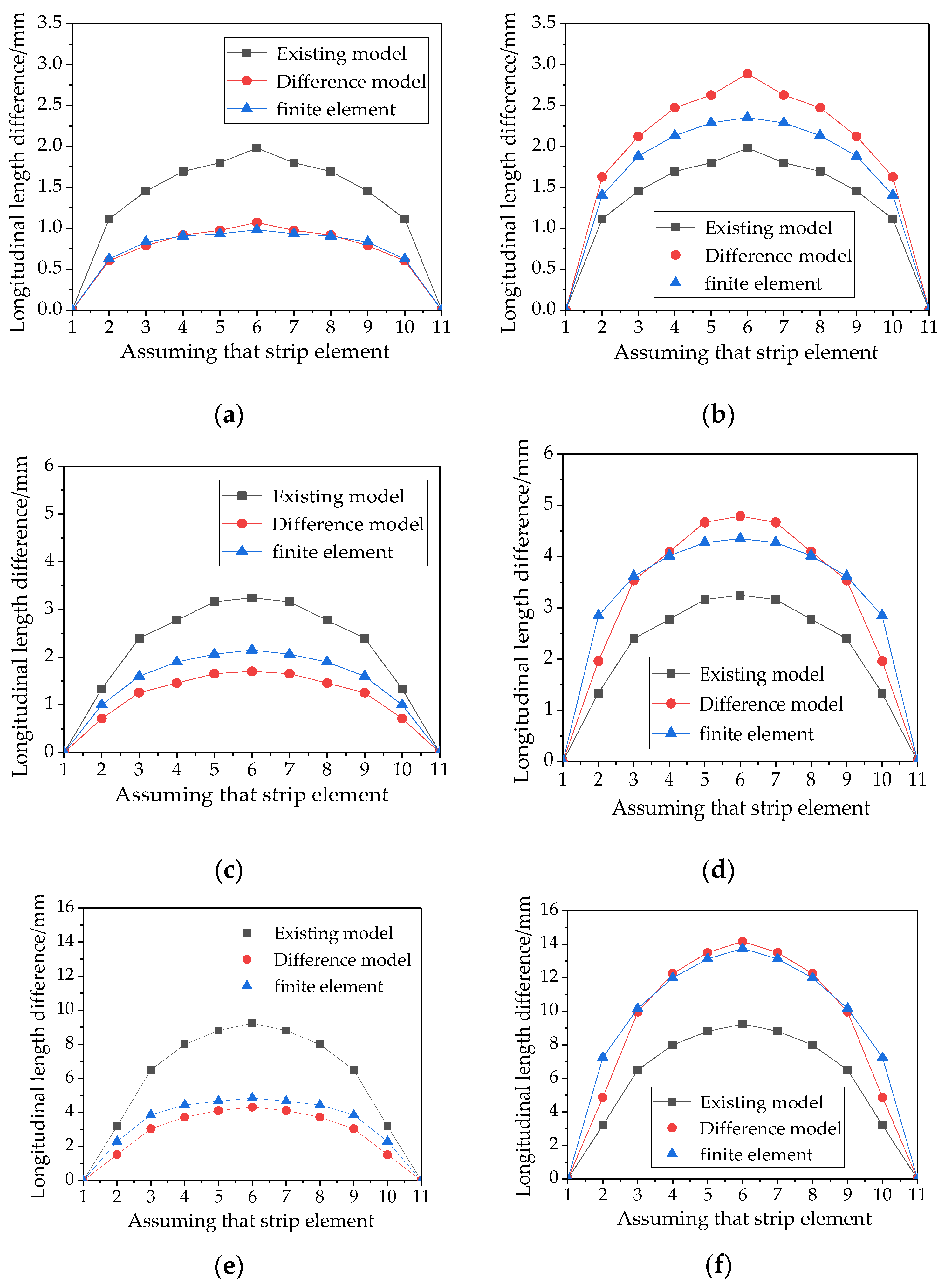
6.1. Finite Element Simulation

Finite element simulation is carried out using a preset rolling process. The important rolling presupposition parameters in the finite element simulation are shown in

Table 3. The table of rolling presupposition parameters.

Project	Parameter
Diameter of roll body (mm)	130
Friction coefficient	0.23
Specimen parameter (mm)	192 × 70 × 16
Number of hypothetical strips	11
The grade and condition of the material	Q345/hot roll

.

The result after 15 passes of rolling is shown in Figure 9.

The workpiece was divided into 11 hypothetical strips along the transverse direction. The plane shape prediction model based on the three-dimensional strip element method was used to calculate the longitudinal length of each strip and predict the plane shape of the preset workpiece [20]. On this basis, the difference mol of the plane shape at the head and tail ends of the workpiece was used to make predictions.

The calculated results of the existing plane shape prediction model, the head and tail end plane shape difference prediction model, and the finite element simulation were compared, as shown in Figure 10.

As seen in Figure 10, the maximum longitudinal length differences at the workpiece ends calculated using the head and tail end plane shape difference prediction model exhibited a high degree of agreement with the simulation result. Based on the data of the maximum longitudinal length differences at the head and tail ends, the coordinates at the endpoints of each hypothetical strip were determined, enabling the prediction of the plane shapes at the workpiece ends. The calculated results of the existing plane shape prediction model, the head and tail end plane shape difference prediction model, and the simulation result were compared, as shown in Figure 11.

Figure 11 presents a comparison of the simulation results and the predicted results for the 5th, 10th, and 15th rolling passes. It can be seen that the calculation result of the model of the plane shape difference at the head and tail ends is similar to the simulation result.

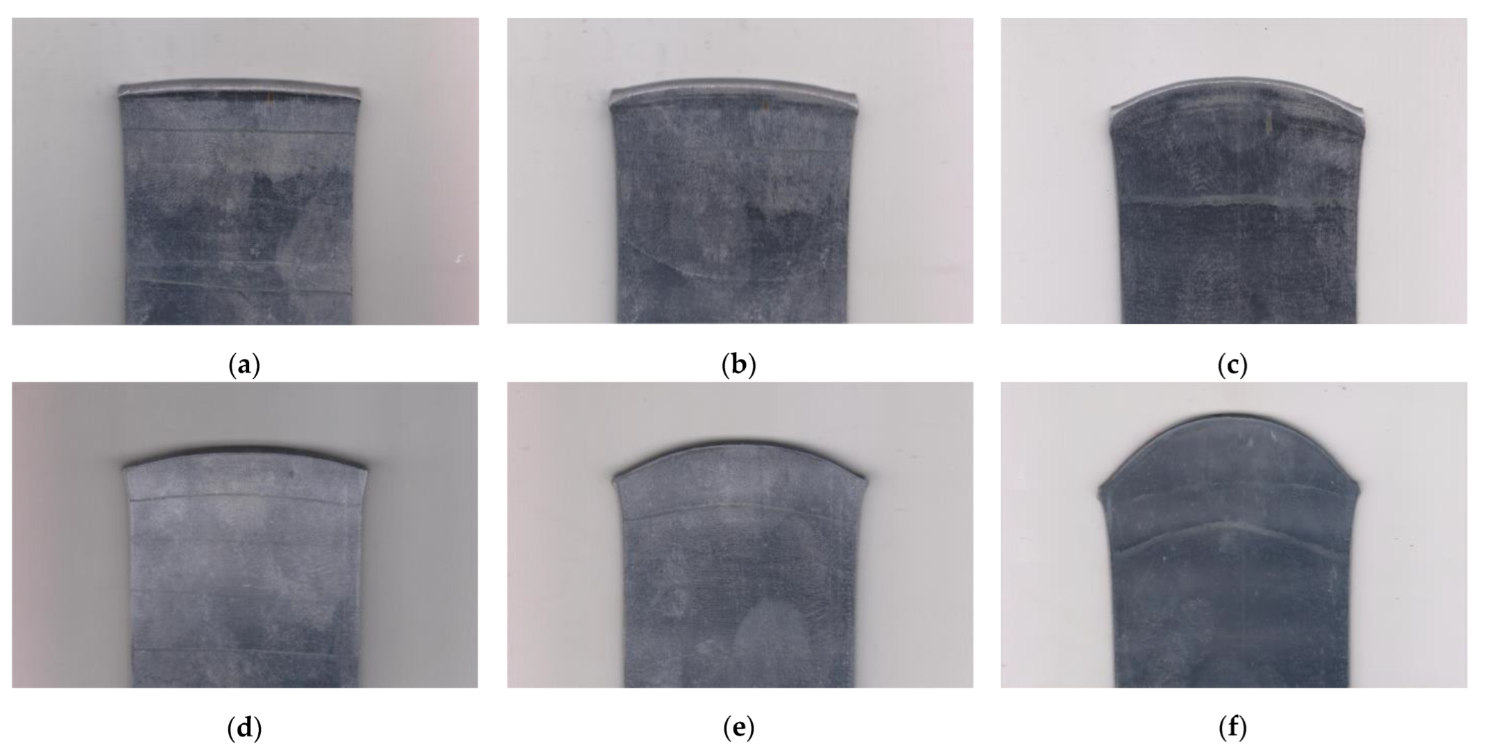
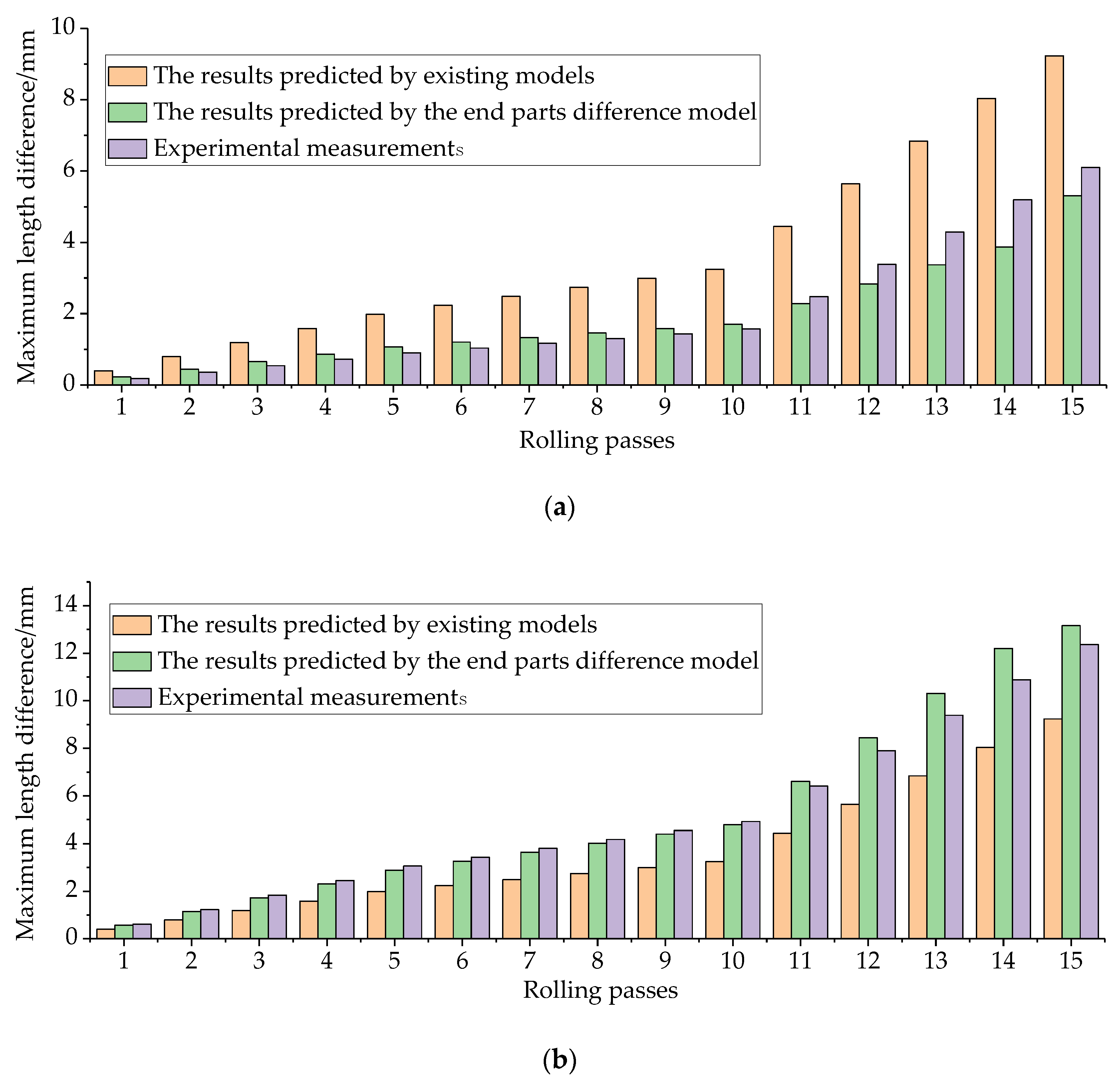
6.2. Rolling Experiment

Considering the similarity of the hot rolling states between lead and low-carbon steel, a series of unidirectional conventional rolling experiments were performed on lead specimens using an experimental rolling mill. The experimental equipment and specimen parameters are shown in

Table 4. The table of rolling process parameters and parameters of the experimental equipment.

Project	Parameter
Type of the rolling mill	Two-high rolling mill
Length of roll body (mm)	260
Diameter of roll body (mm)	110
Friction coefficient	0.11
Specimen parameter (mm)	96 × 70 × 16
Number of hypothetical strips	11
The grade and condition of the material	Lead metal/normal temperature

.

The plane shape of the workpiece can be obtained by the rolling experiment with the preset process, as shown in Figure 12.

The plane shape prediction model based on the three-dimensional strip element method is still applied to calculate the longitudinal length of each strip and predict the plane shape of the preset workpiece, and the differences model of plane shape at the head and tail ends of the workpiece is used to predict.

The maximum longitudinal length differences at the head and tail ends after each rolling pass were determined. The calculated results of the existing plane shape prediction model, the head and tail end plane shape difference prediction model, and the experimental measurements were compared, as shown in Figure 13.

As seen in Figure 13, the maximum longitudinal length differences at the workpiece ends calculated using the head and tail end plane shape difference prediction model exhibited a high degree of agreement with the measured results, and the prediction accuracy was higher than that of the existing plane shape prediction model. The calculated results of the existing plane shape prediction model, the head and tail end plane shape difference prediction model, and the experimental measurements were compared, as shown in Figure 14.

Figure 14 presents a comparison of the measured and predicted results for the 5th, 10th, and 15th rolling passes. The analysis showed that the plane shape data at the workpiece ends obtained using the head and tail end plane shape difference prediction model described in this study exhibited a good degree of agreement with the measured data, and the prediction accuracy significantly improved compared with the existing plane shape prediction model.

7. Conclusions

In this paper, a novel approach for predicting the planar shape differences between the head and tail ends of rolled products has been proposed. The concept of longitudinal length difference in the end sections of rolled products was introduced, and the maximum longitudinal length difference was used as a characteristic representing the planar shape of the product’s ends.

By selecting one-quarter of the metal within the rolling deformation zone as the subject of this study, the paper derived a calculation formula for the metal volume within the forward and backward sliding areas of the rolling deformation zone. This study established a functional relationship between the metal volume in the sliding areas and the longitudinal length difference at the rolled product’s ends using theoretical and experimental research methods.

Using the data on the longitudinal length differences of the end sections of each hypothetical strip, the planar shape curves of the end sections were determined. This enabled the prediction of planar shape differences between the head and tail ends of the rolled products.

The planar shape difference prediction model described in this paper for the head and tail ends of medium-thickness plates is effective in improving prediction accuracy and offers simple and reliable computation. The high correlation between the predicted results and actual measurements makes the model practical and significant for engineering applications.

References

1. Wang, J.; He, C.Y.; Jiao, Z.J. Research and Industrial Practice on Plane Shape Control Model of Medium and Thick Plate; Metallurgical Industry Press: Beijing, China, 2015; pp. 2–21. [Google Scholar]
2. Tan, L.J.; Zhang, S.; Ma, Y.H. Optimization and application of plane shape control model for plate mill. Steel Roll. 2019, 36, 14–17. [Google Scholar]
3. Jiao, Z.J.; He, C.Y.; Ding, J.G.; Wang, J.; Zhang, K.B.; Wang, L.X. Industrial popularization and application of surface shape control technology in plate mill. Iron Steel 2019, 54, 49–55. [Google Scholar]
4. He, H.N.; Shao, J.; Wang, X.C.; Yang, Q.; Liu, Y.; Xu, D.; Sun, Y.Z. Research and application of approximate rectangular section control technology in hot strip mills. Iron Steel Res. Int. 2021, 28, 279–290. [Google Scholar] [CrossRef]
5. Liu, C.; Yuan, Y.; He, A.R.; Wang, F.J.; Sun, W.Q.; Shao, J.; Liu, H.Y.; Miao, R.L.; Zhou, X.G.; Ma, B. Research on the Cause and Control Method of Edge Warping Defect during Hot Finishing Rolling. Metals 2023, 13, 565. [Google Scholar] [CrossRef]
6. Shen, M.; Lu, C.N.; Li, L. Research and application of mathematical model of planar shape control. Steel Roll. 2016, 33, 19–23. [Google Scholar]
7. Li, L.J.; Xie, H.B.; Liu, X.; Liu, T.W.; Wang, E.R.; Jiang, Z.Y. Numerical simulation of strip shape of high-strength steel during hot rolling process. Key. Eng. Mater. 2020, 830, 43–51. [Google Scholar] [CrossRef] [Green Version]
8. Pietschnig, C.; Andreas, S.; Steinboeck, A.; Kugi, A. Are edger rolls useful to control the plate motion and camber in a reversing rolling mill? J. Process Control 2022, 114, 71–81. [Google Scholar] [CrossRef]
9. Ding, X.K.; Yu, J.M.; Zhang, T.H. Establishment of digital model of plane shape of medium and thick plate. Iron Steel 1998, 33, 33–37. [Google Scholar]
10. Yang, Y.B.; Peng, Y. Theoretical model and experimental study of dynamic hot rolling. Metals 2021, 11, 1346. [Google Scholar] [CrossRef]
11. Moon, Y.H.; Chun, M.S.; Yi, J.J.; Kim, J.K. Physical Modelling of Edge Rolling in Plate Mill with Plasticine. Steel Res. Int. 1993, 11, 557–562. [Google Scholar] [CrossRef]
12. Wang, X.W.; Zhang, Y.J.; Guo, Q. Prediction of hot finishing rolling bandwidth based on rolling mechanism and hybrid neural network. China Metall. 2023, 33, 114–120. [Google Scholar]
13. Dong, Z.S.; Li, X.; Luan, F.; Zhang, D.H. Prediction and analysis of key parameters of head deformation of hot-rolled plates based on artificial neural networks. J. Manuf. Process. 2022, 77, 282–300. [Google Scholar] [CrossRef]
14. Schausberger, F.; Steinboeck, A.; Kugi, A. Feedback Control of the Contour Shape in Heavy-Plate Hot Rolling. IEEE Trans. Control. Syst. Technol. 2018, 26, 842–856. [Google Scholar] [CrossRef]
15. Ding, J.G.; Ni, Y.; Sun, L.R.; Li, H.; Li, X.; Zhang, D.H. Width prediction of hot rolling based on density clustering collaborative depth residual network. Metal Ind. Autom. 2022, 36, 67–77. [Google Scholar]
16. Zhao, Y.; Yang, Q.; He, A.R.; Wang, X.C. Research and application of high precision model for predicting plane shape of medium thick plate. Iron Steel 2011, 46, 55–63. [Google Scholar]
17. Jiao, Z.J.; Hu, X.L.; Zhao, Z.; Li, H.T.; Guo, J.F.; Liu, X.H. Online application of surface shape control function of plate mill. Steel Res. 2007, 19, 56–59. [Google Scholar]
18. Yu, J.M.; Li, J.P.; Jing, Q.Z.; Wang, H. Study on deformation law of medium and thick plate plane shape and its measurement. Steel Roll. 1998, 2, 3–7. [Google Scholar]
19. Du, P. Research on Rolling Theory and Control Strategy for Longitudinally Profiled Flat Steel. Ph.D. Thesis, Northeastern University, Shenyang, China, 2008. [Google Scholar]
20. Liu, H.M. Theory and Application of Three Dimensional Rolling; Science Press: Beijing, China, 1999; pp. 55–83. [Google Scholar]
21. Wang, Z.H.; Liu, Y.M.; Wang, T.; Sun, J.; Zhang, T.H. Prediction and analysis of rolling force and wide spread in roughing process. Iron Steel 2022, 57, 95–102. [Google Scholar]
22. Liu, H.M.; Lian, J.C. The study of linear strip element method for metal transverse flow and tension distribution in cold rolled strip. Steel Res. 1992, 4, 37–44. [Google Scholar]
23. Chun, M.S.; Moon, Y.H. Optimization of edging amount for high accuracy plan view control in plate mill. Steel Res. Int. 2001, 72, 17–23. [Google Scholar] [CrossRef]
24. Li, X.; Dong, X.S.; Ding, J.G. Data driven deformation prediction and intelligent optimization of hot rolled steel plate head. Steel Res. 2022, 34, 1398. [Google Scholar]
25. Wang, J.; Chen, F.Q.; Jiang, Y.S.; Wang, Y.J.; Tu, J.; Huang, J.Y. Study on shape symmetry of head, and tail end of wide-thick plates. Steel Roll. 2017, 35, 23–27. [Google Scholar]
Figure 1. Schematic diagram of hypothetical strips’ planar shapes: (a) hypothetical strips’ planar shapes before rolling; (b)hypothetical strips’ planar shapes after rolling.
Metals 13 01123 g001
Figure 2. Schematic diagram of the plane shapes of the head and tail ends of the rolled product: (a) plane shape of the head end of the rolled product; (b) plane shape of the tail end of the rolled product.
Metals 13 01123 g002
Figure 3. Schematic diagram of hypothetical strips’ planar shapes of the end: (a) hypothetical strips’ planar shape before rolling; (b) hypothetical strips’ planar shape after rolling.
Metals 13 01123 g003
Figure 4. The process of predicting differences in planar shapes at the head and tail ends.
Metals 13 01123 g004
Figure 5. Schematic diagram of one-quarter of the metal in the deformation zone.
Metals 13 01123 g005
Figure 6. Schematic diagram of the metal in the backward slip zone.
Metals 13 01123 g006
Figure 7. Comparison of experimental results of rolling specimens: (a) comparison of experimental results at the head end of No. 1 specimen; (b) comparison of experimental results at the head end of No. 2 specimen; (c) comparison of experimental results at the head end of No. 3 specimen; (d) comparison of experimental results at the tail end of No. 1 specimen; (e) comparison of experimental results at the tail end of No. 2 specimen; (f) comparison of experimental results at the tail end of No. 3 specimen.
Metals 13 01123 g007
Figure 8. The relationship between the prediction model of end plane shape difference and the existing plane shape prediction model.
Metals 13 01123 g008
Figure 9. The result of finite element simulation.
Metals 13 01123 g009
Figure 10. Comparison of the shape characteristics of each pass: (a) comparison of the shape characteristics of the head end of each pass; (b) comparison of the shape characteristics of the tail end of each pass.
Metals 13 01123 g010
Figure 11. Comparison of calculation results and simulation results: (a) comparison of the head end after the 5th pass; (b) comparison of the tail end after the 5th pass; (c) comparison of the head end after the 10th pass; (d) comparison of the tail end after the 10th pass; (e) comparison of the head end after the 15th pass; (f) comparison of the tail end after the 15th pass.
Metals 13 01123 g011
Figure 12. The photographs of the results of the experiment: (a) the photograph of the head end after the 5th pass; (b) the photograph of the head end after the 10th pass; (c) the photograph of the head end after the 15th pass; (d) the photograph of the tail end after the 5th pass; (e) the photograph of the tail end after the 10th pass; (f) the photograph of the tail end after the 15th pass.
Metals 13 01123 g012
Figure 13. Comparison of the shape characteristics of the end parts of each pass: (a) comparison of the shape characteristics of the head end of each pass; (b) comparison of the shape characteristics of the tail end of each pass.
Metals 13 01123 g013
Figure 14. Comparison of the plane shapes of the head and tail ends: (a) comparison of the head end after the 5th pass; (b) comparison of the tail end after the 5th pass; (c) comparison of the head end after the 10th pass; (d) comparison of the tail end after the 10th pass; (e) comparison of the head end after the 15th pass; (f) comparison of the tail end after the 15th pass.
Metals 13 01123 g014