Assessment of Porosity Defects in Ingot Using Machine Learning Methods during Electro Slag Remelting Process

Abstract

The porosity defects in the ingot, which are caused by moisture absorption in slag during the electroslag remelting process, deserve the researcher’s attention in the summer wet season. The prediction of slag weight gain caused by moisture absorption is critical for developing slag baking and scheduling strategies and can assist workshop managers in making informed decisions during industrial production of electro slag remelting. The moisture absorption in slag under the conditions of different air humidity, experimental time, slag particle size, and CaO content in the slag are investigated by slag weight gain experiments. The purpose of this study is to predict the rate of weight gain in slag using observed weight gain data and machine learning (ML) models. The observation dataset includes features and rate of weight growth, which serve as independent and dependent variables, respectively, for ML models. Four machine learning models: linear regression, support vector regression, random forest regression, and multi-layer perceptron, were employed in this study. Additionally, parameters for machine learning models were selected using 5-fold cross-validation. Support vector regression outperformed the other three machine learning models in terms of root-mean-square errors, mean squared errors, and coefficients of determination. Thus, the ML-based model is a viable and significant method for forecasting the slag weight gain rate, whereas support vector regression can produce results that are competitive and satisfying. The results of slag weight gain data and ML models show that the slag weight gain increases with the increase of air humidity, experimental time, slag particle size, and CaO content in the slag. The porosity defect in the ingot during the ESR process often appears when the moisture in the slag exceeds 0.02%. Considering saving electric energy, the complexity of on-site scheduling, and 4 h of scheduling time, the slag T3 (CaF₂:CaO:Al₂O₃:MgO = 37:28:30:5) is selected to produce H13 steel ESR ingot in the winter, and slag T2 (CaF₂:CaO:Al₂O₃:MgO = 48:17:30:5) is selected to produce H13 steel ESR ingot in the summer.

1. Introduction

Electroslag remelting (ESR) is utilized to manufacture special steels [1,2] as for its excellent solidification structure and secondary slag refining. It is a significant advantage that good contact between metal and slag makes the steel chemically refined. However, the existence of the slag phase has the disadvantage of controlling the porosity defects in the ingot in the summer wet season due to the moisture absorption in slag. Moisture will be absorbed into slag as a result of the reactions at the slag interface. During the industrial ESR process, the moisture content of the slag plays a significant role in the formation of ESR ingots [3,4,5,6,7,8]. Several investigations [9,10] have shown that moisture may be removed by preheating the slag before ESR, while Polonsky et al. [11] indicated that extensive porosity and defects near sample surfaces are typically much more difficult to eradicate. Although the slags were baked for 12 h at 700 °C before the ESR process, the porosity defects [12,13,14,15] remain in the ESR ingot, as seen in Figure 1. It is the time from taking the slag out of the heating furnace to adding it into the ESR furnace that causes moisture increase in the slag. Furthermore, the heated slag will reabsorb moisture when put in humid air [16,17,18,19,20]. Moisture absorption of heated slag during the period from taking it out of the heating furnace to putting it into the ESR furnace has a large influence on porosity defects of ingot [21,22,23]. Moisture is absorbed into metal or slag as a result of processes at the slag interface. Moisture in ESR slag has been a topic of much discussion on a practical level, but there is a dearth of research on the weight gain prediction of slag in the literature. As far as we know, this is the first study to employ machine learning techniques to design and assess the performance of machine learning algorithms for the prediction of slag weight gain rate, and it is worthwhile evaluating the moisture absorption capacity of heated slag in humid air in advance, using machine learning (ML) techniques to assist the producer in making more precise decisions.

The applications of ML techniques have grown dramatically in recent years, and they are now widely used in a variety of fields. Han et al. [24] and Tandel et al. [25] employed ML methods to voice recognition and speaker recognition. Kaur et al. [26] proposed an ML-based system to accurately categorize the Sunflower flower in its natural habitat with an accuracy of 88.52%. Celli et al. [27] revealed that the ML-based approaches performed well when predicting the personality and interaction features of users’ profile images. Dada et al. [28] recommended using more advanced ML methods, such as deep learning techniques, to combat email spam. Choi and Lim [29] identified that the ML-based strategies may also be utilized to safeguard adviser interests. Even in the sphere of healthcare, ML-based strategies have been widely implemented. Karaman et al. [30] constructed a convolutional neural networks model to automate the detection of Parkinson’s disease with a high degree of accuracy. Notably, Alhudhaif et al. [31] and Polat et al. [32] employed ML techniques to diagnose the new coronavirus disease 2019 (COVID-19), which sped up the COVID-19 diagnosis and saved crucial time for disease control. ML is a subfield of computer science concerned with the study of algorithms capable of learning from and generalizing on data. Within ML, there are two primary paradigms: regression and classification [33]. Regression entails the collection of input variables and predicting the value of the output (dependent) variable(s). It is based on forecasting a numeric value by estimating the connections between variables (independent and dependent variables) (with an associated variance, in some cases). On the other hand, classification refers to the process of accepting input variables and determining which of the N classes they belong to, using training data from exemplars of each class. In this respect, it is based on the discovery of decision boundaries that are suitable for separating the various classes.

ML algorithms may “learn” complicated relationships between predictors and the target variable, as well as interactions between predictors, without requiring the underlying model to be specified [34]. ML also caught the attention of the steel sector [35,36,37]. Hence, it is an intriguing study topic if ML techniques enable superior moisture absorption of heated slag decisions. We address this challenge by studying ML techniques for a highly relevant issue in active portfolio management: slag weight gain rate (SWGR) predictions in the humid air.

As previously stated, the purpose of this work is to predict the SWGR using a regression model constructed from training data. Regression analysis is a statistical procedure that involves the construction of mathematical models between dependent and independent variables [38]. With regression analysis, one may determine the relationship that exists between input and output while controlling for other independent factors. For machine learning regression analysis, the objective is to map the relationship between inputs referred to as features and continuous numeric values as predictors. ML-based regression algorithms will be beneficial for a range of applications. Linear regression (LR) [39], support vector machine regression (SVR) [40,41], random forest regression (RFR) [42,43], and multi-layer perceptron (MLP) [44] models are all frequently used ML regression approaches, and they are also employed in this study.

This paper is organized as follows: Section 2 describes the research process, SWGR experiment design, and the ML methods employed in this study. Section 3 presents the results and discussion of the experiment described in Section 2.1 and the performance assessment of the machine learning methods used to predict the SWGR. Finally, Section 4 describes the conclusions of this study.

2. Experiments and Machine Learning Methods

In accordance with Figure 2, the proposed approach is separated into several stages.

The first step was to conduct an experiment on slag weight gain in humid air and to record the results in a database, and this step was carried out with the assistance of several specialists. The second step in our methodology is data preprocessing, during which the data is normalized to standardize the units of measurement and therefore enable data comparison. Following the preprocessing step, the prediction step employed four machine learning algorithms, and the prediction models were trained using 5-fold cross-validation. The RMSE, MSE, and R² values were utilized to compare the performance of SWGR prediction accuracy during the assessment step.

2.1. Slag Weight Gain in Humid Air Experiment Design

In this section, the slag weight gain experiment is presented. In the slag weight gain experiment in humid air, three kinds of pre-melted slag containing different amounts of CaO are used, and the composition of slag is listed in

Table 1. Composition of pre-melted slag used in weight gain experiment.

Slag.	CaO (%)	CaF2 (%)	Al2O3 (%)	MgO (%)
T1	5	60	30	5
T2	17	48	30	5
T3	28	37	30	5

.

The experimental device used for slag weight gain is shown in Figure 3. It can be seen that the slags were contained in the petri dishes, and the water was heated by the constant temperature water generator. In addition, the sensors used in this experiment have a high degree of accuracy; in particular, the hygrometer sensor has a range of 10–99% and a measurement accuracy of ±(2–3%), and the highly precise electronic scale has a weight limit of 320 g and a measurement accuracy of 0.001 g.

The following describes the experimental procedure: (i) The pre-melted slags are processed into different particle sizes; (ii) The slags were heated for 12 h at 700 °C to fully remove moisture before experiments; (iii) The 100 g heated slags were put into the experimental device described in Figure 3 for 4, 8, 16, 32 h; (iv) The weight gain values of slags in each experiment were measured by high precision electronic scale. Following the experiments, Figure 4 summarizes the experimental settings and corresponding weight gain rate results.

2.2. Dataset Description

The data were collected from actual observed data of the experiment mentioned in Section 2.1. The SWGR served as the objective of this study, and four independent variables were used as inputs to predict the SWGR. To model and assess SWGR prediction, this study employed a total of 72 data observations from the experiment. The experiment dataset was separated into training and test subsets. In general, for the purpose of SWGR prediction, the test dataset consisted of 15 points (20% of the dataset), whereas the training dataset comprised 57 points of 72 records (80% of the dataset).

The variables employed in this study are listed in

Table 2. Description of variables and the PCC.

Types of Variables	Attribute Name	Description	PCC
Independent variables	X1	Slag particle size	0.371
	X2	CaO %	0.563
	X3	Humidity	0.353
	X4	Placement time	0.406
Dependent variable	Y	Weight gain rate	-

. Additionally, the Pearson correlation coefficient (PCC) [45] was employed to determine which independent variables had a significant correlation coefficient with the SWGR. The PCC column in Table 2 describes the relationship between the independent variables and the SWGR variable. The PCC findings indicate that the quantity of CaO in the slags has a greater effect on the SWGR than the other independent variables, whereas humidity and slag particle size have a similar effect. Furthermore, the statistical information is summarized in

Table 3. Statistics information for the dependent variable and independent variables.

	X1	X2	X3	X4	Y
Mean	61.67	16.67	66.00	15.00	0.027
Std.	29.16	9.46	12.08	10.80	0.029
Min	30.00	5.00	54.00	4.00	0.001
Max	100.00	28.00	78.00	32.00	0.150

.

Standardization was used to preprocess the dataset’s characteristics. This step is critical because the attributes in the dataset obtained had varying scales. Standardizing the data allowed for the adjustment of these values to a similar condition. The MinMax approach was employed in this study to transform attribute values into [0, 1] scaled values, as described in Equation (1).

$$x^{\prime }=\frac{x-min\left(x\right)}{max\left(x\right)-min\left(x\right)}$$

(1)

where x is the relevant variable.

2.3. Machine Learning Methods

Four machine learning models for predicting and analyzing SWGR were developed in Python (version 3.8, Python Software Foundation, Beaverton, OR, USA) using the scikit-learn (version 0.24) [46] package. The ML experimental setup comprised of a 2.9 GHz Intel Core i7 node with 16 Gb ram. Since the dataset in this study is relatively limited, only the central processing unit (CPU) was used to train all ML models. The employees recorded experimental data such as slag particle size, CaO percent, humidity, and placement time (in hours). The critical phase in data preprocessing is determining which models to attempt to fit the data. The study’s problem is a single-output regression-type machine learning problem. Single-output regression is used to describe situations involving the prediction of a single numerical value given a set of input samples. Numerous machine learning algorithms have been developed to predict a single numeric number. The following models were chosen for this study due to their ease of implementation using the scikit-learn package and their popularity in real-world data fitting situations. Each of the four models was trained independently using the same training data and was evaluated using the same testing data.

2.3.1. Linear Regression (LR)

By minimizing the residual sum of squares between the observed and anticipated data, linear regression is used to build a model with coefficients [33]. It is used to examine if a dependent variable and one or more independent variables have a linear relationship. The purpose of this study was to construct a linear regression method and to fit a model using the training data. After training, the model was validated using the test sub-dataset to evaluate the performance of prediction accuracy.

2.3.2. Support Vector Regression (SVR)

SVR is a kind of supervised machine learning algorithm based on statistical learning theory [47]. In comparison to the linear regression method, SVR is effective in modeling nonlinearly related features and solving regression tasks. SVR is a popular machine learning approach that is utilized in numerous applications [48,49]. One of the reasons for SVR’s widespread utilization is that it makes use of kernels. A kernel is a function that maps the feature vectors to a higher dimension, allowing features that are not linearly separable in lower dimensions to become separable. Kernels are very beneficial when dealing with complex and nonlinear tasks. The linear, polynomial, radial basis function (RBF), and sigmoid kernels are all types of SVR kernels [47]. The RBF kernel with a value of 0.15 was employed in this study.

2.3.3. Random Forests Regression (RFR)

Random forest or random decision forest is an ensemble learning method for classification, regression, and other tasks [50]. It works by building a lot of decision trees (DTs) at training time and then outputting the class that is the mode of the classes or the mean prediction of the individual trees. In this study, the RFR scikit-learn estimator was built, trained, and tested with the datasets used in this study. There are nodes, branches, and leaves in the structure of a DT model. The nodes are features or predictors, and the branches are decisions. The leaves are responses or outputs. Regression DT can output continuous values that can be used to model SWGR. This RFR can fit data, make predictions quickly, and use very little memory.

2.3.4. Multi-Layer Perceptron (MLP)

Artificial neural networks, colloquially referred to as neural networks, are inspired by the structure and operation of the human brain’s nervous system. Their objective is to elucidate the enigma of human intelligence via the examination of the human brain’s composition mechanism and way of thought [51]. Neurons are the fundamental building blocks of neural networks, and the connecting of a large number of neurons in a neural network generates a variety of intelligent actions. Each neuron can receive a set of input signals from other neurons, each input representing a weight, and the neuron’s output is determined by the weighted sum of all inputs. There are several techniques to link neurons in neural networks. Different connecting mechanisms result in a variety of network connection models. The multi-layer perceptron (MLP) is a type of neural network that consists of numerous hidden layers linked by neurons [52]. MLP is often utilized as a feed-forward supervised neural network and is frequently used due to its simple design, rapid operation, ease of construction, and ability to solve complex classification tasks. Three primary layers comprise the MLP system: an input layer, a hidden layer, and an output layer. These three primary layers are employed for data intake, data transport, and data output. The hidden layer’s purpose is to send the results to the output layer. Each neuron’s output can be scientifically characterized as given in Equation (2):

$$y_i=f\left({\sum }^{ }{w}_{ij}{x}_i\right)$$

(2)

where $y_i$ is the input that a single node $j$ receives. The function $f$ is a threshold, sigmoid, or hyperbolic tangent function. $w_{ij}$ denotes the weights between nodes $i$ and $j$, while $x_i$ denotes the output from node $i$.

2.4. Cross Validation

Both ML methods and regularized linear models rely on the selection of “tuning parameters” [53,54]. In essence, these parameters specify the degree to which a model adapts to the training data. Tuning parameters include, but are not limited to, the penalization parameter in linear regression, as well as the number or depth of trees in the random forest and boosting. Tuning parameters can be adjusted to extreme values, resulting in a model that is complicated and adapts nearly flawlessly to the training data. However, models that are extremely well-adapted to the training data are frequently “overfitted”, meaning they perform badly out-of-sample on the data from the test set [55]. This is especially true when the data has a high level of noise, as is the situation with equity market forecasts. To avoid overfitting models, we employ the standard technique of “cross-validation”. Cross-validation is a technique for simulating an out-of-sample test of the model. The N-fold cross-validation divides the training set into N randomly chosen subsets, with ($N-1$) subsets used for training and the remaining subset used for validation. The final model is tuned using the parameters that minimize the forecast error over the n validation sets. All models undergo five-fold cross-validation, and “tuning parameters” are estimated directly from the data.

2.5. Evaluation Metrics

After proposing a set of models, evaluation metrics for the models were provided to compare their performance. The implemented models were evaluated using root-mean-square errors (RMSE), mean squared errors (MSE), and coefficients of determination (R²) [56]. RMSE is one of the most commonly used statistics for estimating prediction error. The MSE statistic is another type of statistical indicator that is used to quantify the absolute error between observed and anticipated values. R² denotes the degree to which the expected and observed data are linearly related. The lower the MSE score, the more accurate the prediction outcomes are. The R² is a percentage value that indicates how much the dependent variable varies in a regression model. These three indices are frequently used to assess the predictive performance of models in the field of regression issues. The equations of these three methods are defined in (3)–(5), $Y_i$ is the actual value and ${\widehat{Y}}_i$ is the forecast value, where $\overline{Y}$ is the mean of the observations and $\tilde{Y}$ is the mean of the prediction, and N is the size of the test data.

$$\mathrm{MSE}={\sum }_{i=1}^N{(Y_i-{\widehat{Y}}_i)}^2$$

(3)

$$\mathrm{RMSE}=\sqrt{\frac{{\sum }_{i=1}^N{(Y_i-{\widehat{Y}}_i)}^2}{N}}$$

(4)

$${\mathrm{R}}^2=\frac{{({\sum }_{i=1}^N(Y_i-\tilde{Y})(Y_i-\overline{Y}))}^2}{{\sum }_{i=1}^N{(Y_i-\tilde{Y})}^2{\sum }_{i=1}^N{(Y_i-\overline{Y})}^2}$$

(5)

3. Results and Discussion

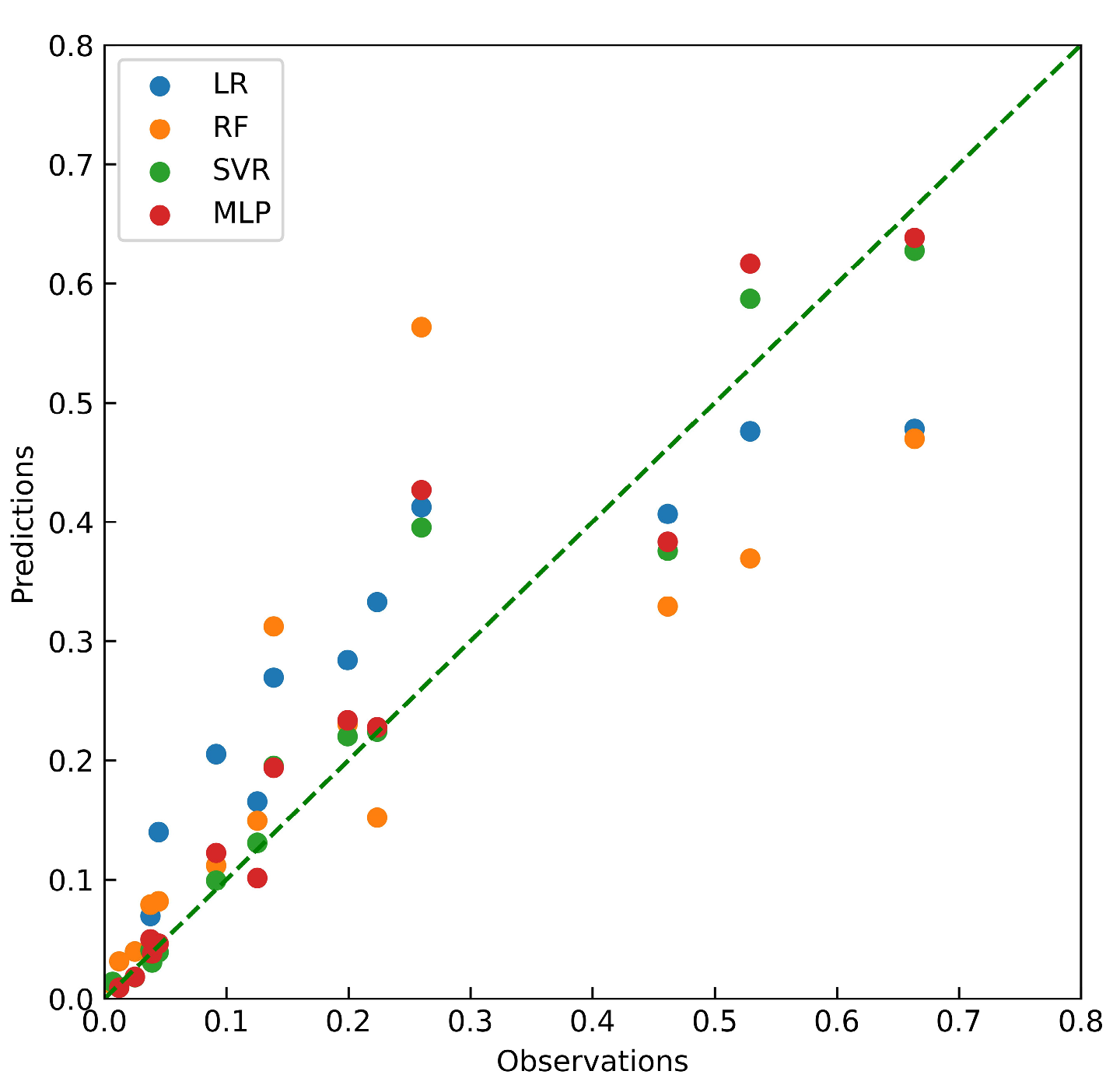
3.1. Prediction of Weight Gain Rate by Machine Learning Methods

This section compares four models (LR, RF, SVR, and MLP) using three metrics: RMSE, MSE, and R². We trained and tested the models using 5-fold cross-validation, and the end results are the metric’s average values.

Table 4. Performance evaluation of proposed regression models.

Model	RMSE	MSE	R2
LR	0.1009	0.0112	0.2717
RF	0.0753	0.0062	0.7229
SVR	0.0270	0.0008	0.9545
MLP	0.0371	0.0023	0.9326

summarizes the performance of the proposed methodologies in predicting the SWGR. As shown in Table 4, SVR performs the best in terms of MSE and R² (R² = 0.9545), MLP follows closely behind (R² = 0.9326), while LR performs the lowest (R² = 0.2717). To gain a better understanding of the models’ performance, plots of anticipated outputs versus actual observations are constructed for the test dataset (14 points), as illustrated in Figure 5. The ideal scenario in this plot would be for all points to lie on a straight line with a slope of 1, indicating that all predictions are identical to observations. As seen in Figure 5, the SVR and MLP models outperform the other models in terms of visual results. As shown in Table 4, the SVR (R² = 0.9545, RMSE = 0.0008) and MLP (R² = 0.9326, RMSE = 0.0371) performed similarly to and better than other models, owing to their higher R² scores and lower RMSE and MSE values. MLP typically performs better than other machine learning approaches because it can learn non-linear and complicated behaviors extraordinarily well. Due to the SVR’s similarity to the MLP, it may be used to generate accurate predictions regarding the SWGR issue. On the other hand, the poor performance of the LR (R² = 0.2717, RMSE = 0.1009) model for SWGR prediction implies that the SWGR and independent variables exhibit non-linear and complicated behaviors. Additionally, the performance of SVR against MLP demonstrates that the use of artificial neural network-based algorithms should not be the sole machine learning approach, and classic machine learning algorithms may do quite well in some sectors.

As shown in Figure 6, the SVR model was used to predict the change in slag weight gain rate with storage time in humid air under different conditions. It is clear that the predicted results in Figure 6 are in good agreement with the measured data in Figure 4. Additionally, Figure 6a demonstrates that the smaller the slag particle size, the greater the slag gains weight. As seen in Figure 6b, the weight gain rate of slag increases as its CaO concentration increases. Figure 6c demonstrates that air humidity has a significant effect on the moisture absorption of heated slag during the transition from the heating furnace to the ESR furnace, which plays a significant role in the ingot’s porosity defects. Summer’s humid environment is a significant contributor to ingot defects.

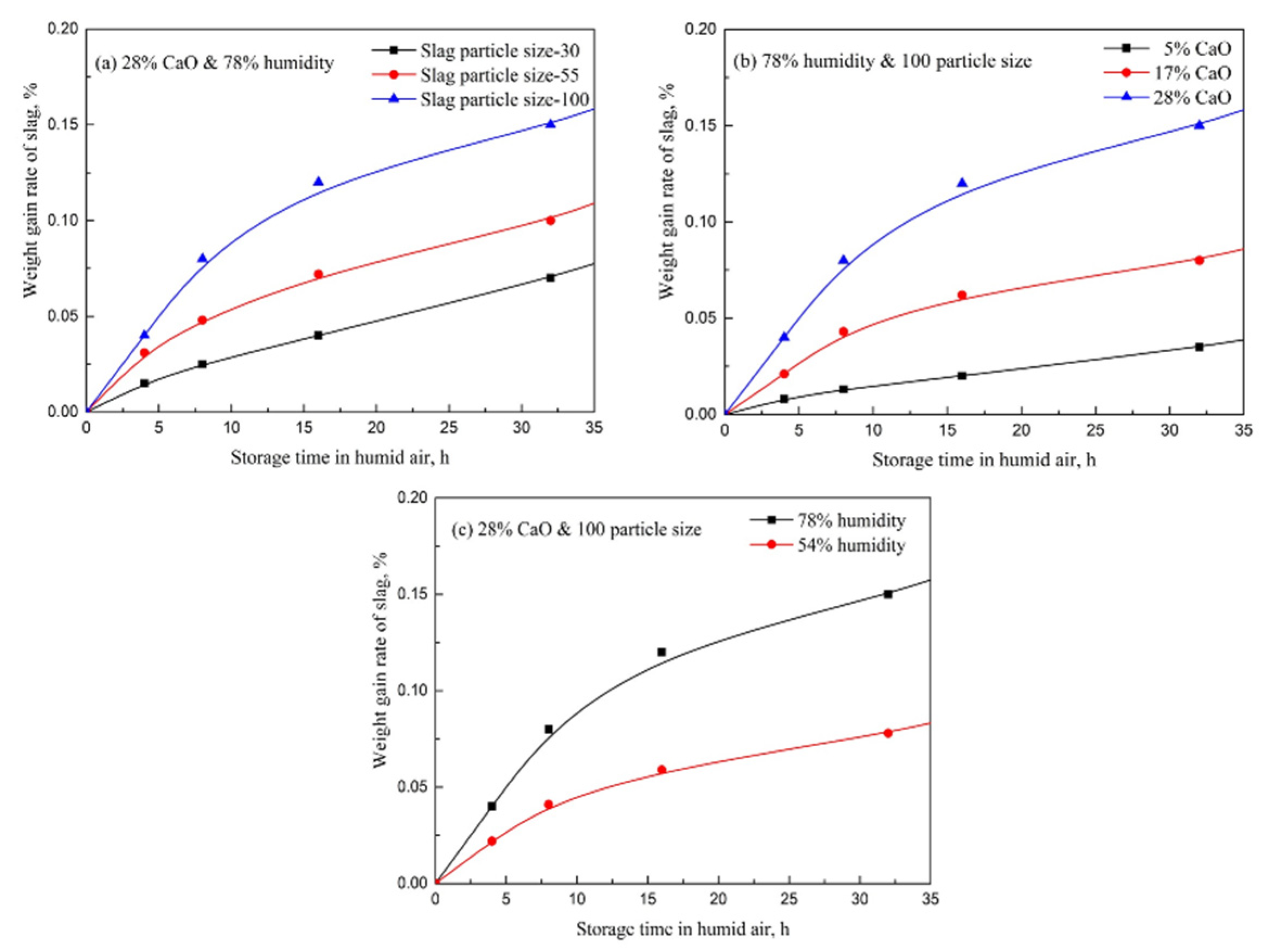
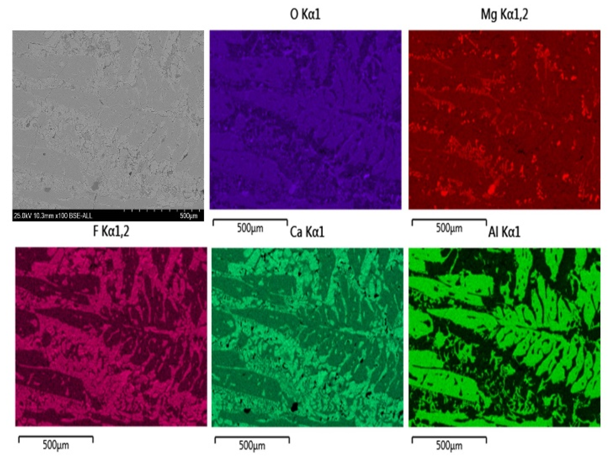
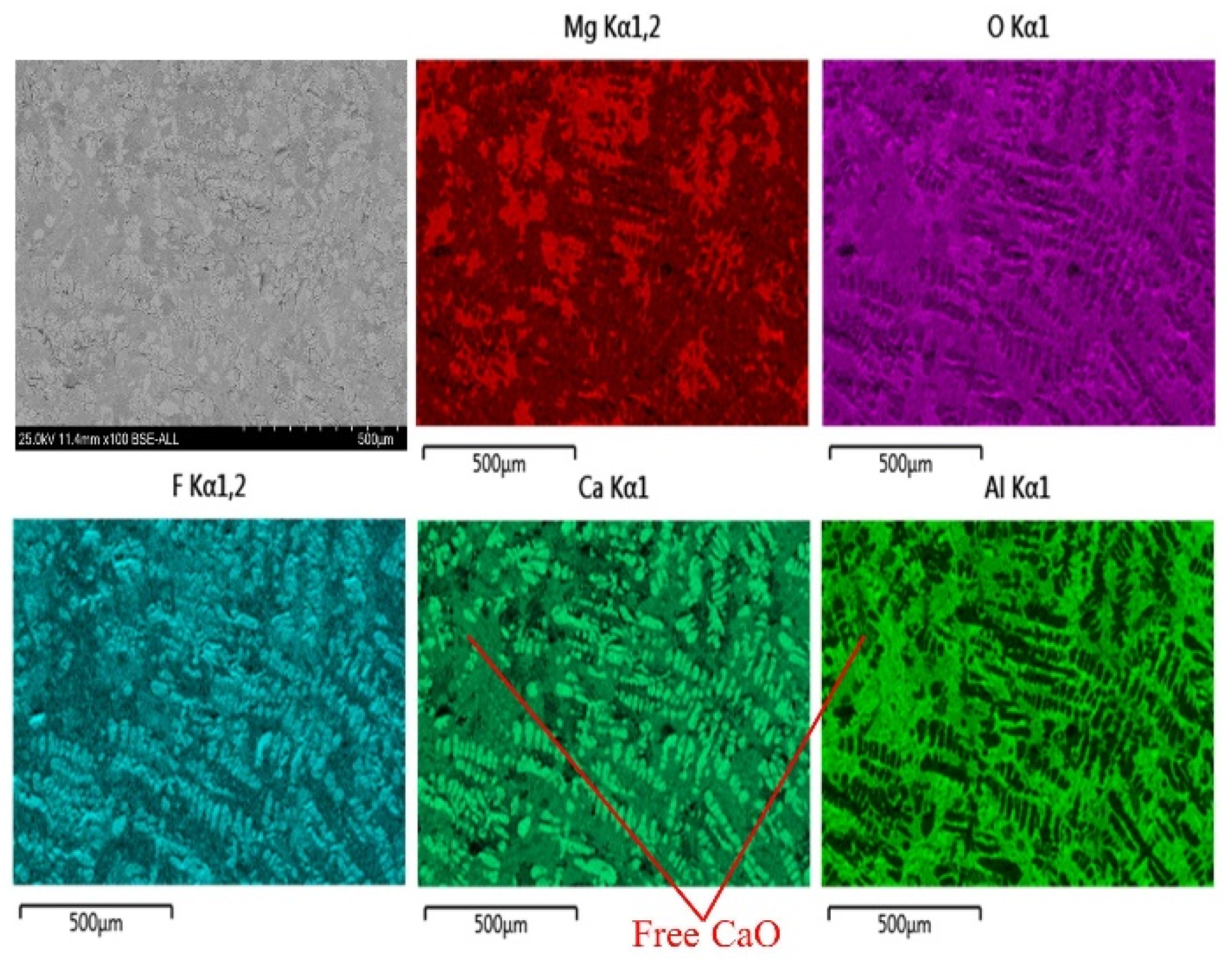
3.2. Analysis of Reasons for Slag Weight Gain

The primary cause of slag weight gain in humid air is the reaction CaO(s) + H₂O(g) = Ca(OH)₂(s). After the slags were pre-melted, the CaO in the slags can form Ca_xAl_yO_z compound with Al₂O₃, which can effectively prevent free CaO from combining with H₂O. T1 contains 5% CaO and T2 contains 17% CaO, there is almost no free CaO in these slags, and existing much Ca_xAl_yO_z in slag systems, the slag weight increases slowly, as shown in Figure 6b. T3 contains 28% CaO, and the existing free CaO caused the rapid increase rate of slag weight.

In order to verify whether there is free CaO in each kind of slag, the element distribution of slag T1, T2, and T3 is analyzed by a scanning electron microscope (SEM) equipped with an energy dispersive spectrometer (EDS), and the results are shown in Figure 7, Figure 8 and Figure 9, respectively. It is clear that: (i) slag T1 without free CaO has a very low rate of slag weight gain; (ii) with the appearance of free CaO in slag T2, the slag weight gain rate is higher than that of slag T1; (iii) slag T3 with a large amount of free CaO has the very high rate of slag weight gain. With the increase of CaO in slag, the formation of Ca_xAl_yO_z is not enough to eliminate all free CaO, which causes the increase in slag weight gain rate.

3.3. Application of Machine Learning Methods

The prediction of the SWGR and the reasons for weight gain were analyzed by machine learning methods and SEM-EDS in the previous sections, respectively. In order to make better use of the machine learning results, the ideal placement time before the pre-heated slags can be put into the ESR process was estimated using the trained SVR model in order to improve efficiency. The 5-ton ESR experimental results of electro slag remelting for one year under different kinds of slag with 100 particle size are summarized in

Table 5. Porosity defects in ingots during ESR process under different seasons and slag system.

Slag.	Steel	Moisture Absorption Time (h)	Season in Coastal Areas	Atmospheric Humidity	Porosity in Ingot	Power Consumption per Ton Steel kW·h
T1	H13	38	Winter	43%	Yes	1490
T1	H13	33	Winter	43%	No	1500
T1	H13	16	Summer	78%	Yes	1470
T2	H13	15	Winter	43%	No	1240
T2	H13	5	Summer	78%	Yes	1220
T3	H13	5	Winter	43%	Yes	950

Notes: Moisture absorption time is the time from taking the slag out of the heating furnace to adding it into the ESR furnace.

. The pre-melted slags were baked for 12 h at 700 °C before the ESR process. The power consumption per ton of steel under the condition of slag T1, T2, and T3 are 1470~1500 kW h, 1220~1240 kW h, and 950 kW h, respectively. Slag T3 is more conducive to saving electric energy. According to the data statistics in Table 5 and the experiments on slag weight gain, the porosity defect in the ingot during the ESR process often appears when the SWGR exceeds 0.02%. Thus, with the trained SVR-SWGR model, the target value was set to 0.02, and the slag placement time between being taken out of the heating furnace and added into the ESR furnace is calculated under different conditions, as shown in

Table 6. Prediction of porosity defects in ingots analyzed by machine learning methods.

Slag.	Steel	Moisture Absorption Time (h)	Season in Coastal Areas	Atmospheric Humidity	Porosity in Ingot
T1	H13	>36	Winter	43%	Yes
T1	H13	>16	Summer	78%	Yes
T2	H13	>18	Winter	43%	Yes
T2	H13	>4	Summer	78%	Yes
T3	H13	>5	Winter	43%	Yes
T3	H13	>1.5	Summer	78%	Yes

.

Table 6 shows that if the placement time is less than 5 h in winter, all three kinds of slags can avoid the porosity defect in the ingot. The slag T3 will most likely cause a porosity defect in the ingot if the placement time is more than 1.5 h in summer. Considering the complexity of on-site scheduling and 4 h of scheduling time, all three kinds of slag can be used to produce an ESR of H13 steel in the winter, and it is forbidden to use slag T3 to produce an H13 die steel ESR ingot in the summer. From the aspects of saving electric energy and product quality, the slag T3 is selected to produce H13 steel ESR ingot in the winter, and slag T2 is selected to produce H13 steel ESR ingot in the summer.

4. Conclusions

Moisture absorption of heated slag during the period from taking it out of the heating furnace to putting it into the ESR furnace plays an important role in the porosity defects of the ingot. This research investigates the slag weight gain in humid air by using four machine learning models. The conclusions are as follows:

(1)

The porosity defect in the ingot during the ESR process often appears when the moisture in the slag exceeds 0.02%. Considering saving electric energy, the complexity of on-site scheduling, and 4 h of scheduling time, the slag T3 (CaF₂:CaO:Al₂O₃:MgO = 37:28:30:5) is selected to produce H13 steel ESR ingot in the winter, and slag T2 (CaF₂:CaO:Al₂O₃:MgO = 48:17:30:5) is selected to produce H13 steel ESR ingot in the summer.

(2)

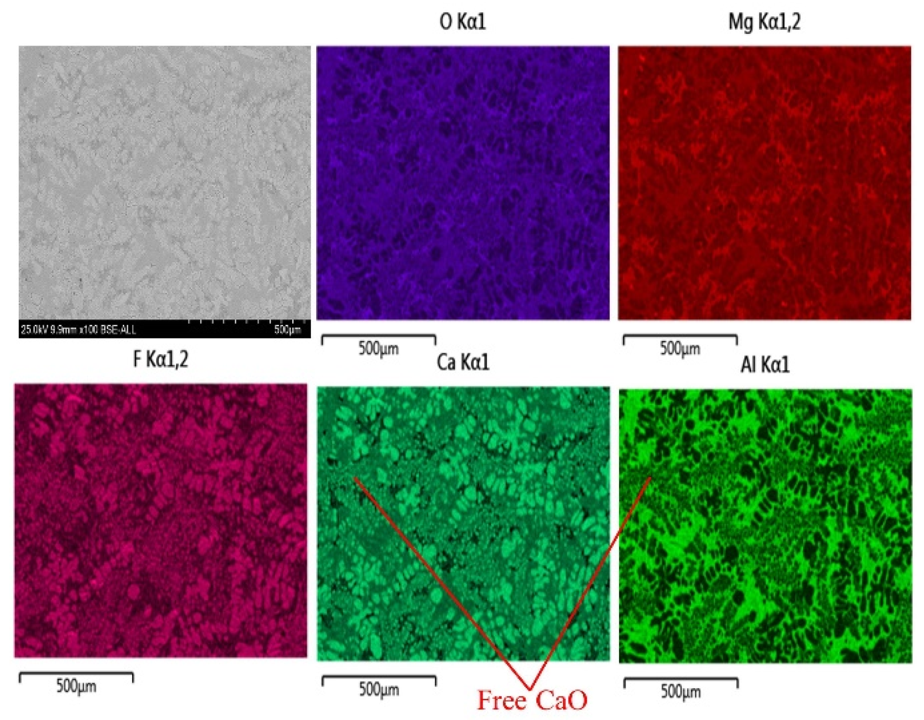
The weight gain rate of slag increases with the increase of air humidity and CaO content in slag. The smaller the slag particle size is, the greater the weight gain rate of slag is. Free CaO in slag makes the air humidity have a large influence on the slag weight gain rate.

(3)

The SVR model can be used to make accurate predictions about “slag weight gain in humid air”, and the calculated results of the SVR model agree well with the measured data.

In the future, machine learning techniques such as deep learning models will be used to assist in strengthening the steel industry’s management capability.

References

1. Shi, C.B.; Li, J.; Cho, J.W.; Jiang, F.; Jung, I.H. Effect of SiO2 on the crystallization behaviors and in-mold performance of CaF2-CaO-Al2O3 slags for drawing-ingot-type electroslag remelting. Metall. Mater. Trans. B 2015, 46, 2110–2120. [Google Scholar] [CrossRef] [Green Version]
2. Duan, S.C.; Shi, X.; Wang, F.; Zhang, M.C.; Sun, Y.; Guo, H.J.; Guo, J. A review of methodology development for controlling loss of alloying elements during the electroslag remelting process. Metall. Mater. Trans. B 2019, 50, 3055–3071. [Google Scholar] [CrossRef]
3. Chen, Z.Y.; Yang, S.F.; Qu, J.L.; Li, J.S.; Dong, A.P.; Gu, Y. Effects of different melting technologies on the purity of superal-loy GH4738. Materials 2018, 11, 1838. [Google Scholar] [CrossRef] [PubMed] [Green Version]
4. Fang, J.L.; Pang, Z.G.; Xing, X.D.; Xu, R.S. Thermodynamic properties, viscosity, and structure of CaO-SiO2-MgO-Al2O3-TiO2-based slag. Materials 2021, 14, 124. [Google Scholar] [CrossRef] [PubMed]
5. Lee, S.H.; Min, D.J. A novel electrochemical process for desulfurization in the CaO-SiO2-Al2O3 system. Materials 2020, 13, 2478. [Google Scholar] [CrossRef]
6. Gao, Y.X.; Leng, M.; Chen, Y.F.; Chen, Z.C.; Li, J.L. Crystallization products and structural characterization of CaO-SiO2-based mold fluxes with varying Al2O3/SiO2 ratios. Materials 2019, 12, 206. [Google Scholar] [CrossRef] [Green Version]
7. Leng, M.; Lai, F.F.; Li, J.L. Effect of cooling rate on phase and crystal morphology transitions of CaO-SiO2-based systems and CaO-Al2O3-based systems. Materials 2019, 12, 62. [Google Scholar] [CrossRef] [Green Version]
8. Gu, S.P.; Wen, G.H.; Ding, Z.Q.; Tang, P.; Liu, Q. Effect of shear stress on isothermal crystallization behavior of CaO-Al2O3-SiO2 -Na2O-CaF2 Slags. Materials 2018, 11, 1085. [Google Scholar] [CrossRef] [Green Version]
9. Bandyopadhyay, T.R.; Rao, P.K.; Prabhu, N. Behavior of alloying elements during electro-slag remelting of ultrahigh strength steel. Metall. Min. Ind. 2012, 4, 6–16. [Google Scholar]
10. Jiang, Z.; Dong, Y.; Liang, L.; Li, Z. Hydrogen pick-up during electroslag remelting process. J. Iron Steel Res. Int. 2011, 18, 19–23. [Google Scholar] [CrossRef]
11. Polonsky, A.T.; Echlin, M.P.; Lenthe, W.C.; Dehoff, R.R.; Kirka, M.M.; Pollock, T.M. Defects and 3D structural inhomogeneity in electron beam additively manufactured inconel 718. Mater. Charact. 2018, 143, 171–181. [Google Scholar] [CrossRef]
12. Jiang, Z.H.; Hou, D.; Dong, Y.W.; Cao, Y.L.; Cao, H.B.; Gong, W. Effect of slag on titanium, silicon and aluminum content in superalloy during electroslag remelting. Metall. Mater. Trans. B 2016, 47, 1465–1474. [Google Scholar] [CrossRef]
13. Hou, D.; Jiang, Z.H.; Dong, Y.W.; Cao, Y.L.; Cao, H.B.; Gong, W. Thermodynamic design of electroslag remelting slag for high titanium and low aluminium stainless steel based on IMCT. Ironmak. Steelmak. 2016, 43, 517–525. [Google Scholar] [CrossRef]
14. Hou, D.; Jiang, Z.H.; Dong, Y.W.; Gong, W.; Cao, Y.L.; Cao, H.B. Effect of slag composition on the oxidation kinetics of al-loying elements during electroslag remelting of stainless steel: Part-2 control of titanium and aluminum content. ISIJ Int. 2017, 57, 1410–1419. [Google Scholar] [CrossRef] [Green Version]
15. Hou, D.; Jiang, Z.H.; Dong, Y.W.; Gong, W.; Cao, Y.L.; Cao, H.B. Effect of slag composition on the oxidation kinetics of al-loying elements during electroslag remelting of stainless steel: Part-1 mass-transfer model. ISIJ Int. 2017, 57, 1400–1409. [Google Scholar] [CrossRef] [Green Version]
16. Hou, D.; Jiang, Z.H.; Qu, T.P.; Wang, D.Y.; Liu, F.B. Aluminum, titanium and oxygen control during electroslag remelting of stainless steel based on thermodynamic analysis. J. Iron Steel Res. Int. 2019, 26, 20–31. [Google Scholar] [CrossRef]
17. Hou, D.; Wang, D.Y.; Qu, T.P.; Tian, J.; Wang, H.H. Kinetic study on alloying element transfer during an electroslag re-melting process. Metall. Mater. Trans. B 2019, 50, 3088–3102. [Google Scholar] [CrossRef]
18. Hou, D.; Wang, D.Y.; Jiang, Z.H.; Qu, T.P.; Wang, H.H.; Dong, J.W. Investigation on slag-metal-inclusion multiphase reac-tions during electroslag remelting of die steel. Metall. Mater. Trans. B 2021, 52, 478–493. [Google Scholar] [CrossRef]
19. Hong, L.; Chen, W.P.; Hou, D. Kinetic analysis of spinel formation from powder compaction of magnesia and alumina. Ceram. Int. 2020, 46, 2853–2861. [Google Scholar] [CrossRef]
20. Hou, D.; Jiang, Z.H.; Dong, Y.W.; Li, Y.; Gong, W.; Liu, F.B. Mass transfer model of desulfurization in the electroslag re-melting process. Metall. Mater. Trans. B 2017, 48, 1885–1897. [Google Scholar] [CrossRef]
21. Liu, W.H.; Li, H.; Zhu, H.M.; Xu, P.J. Effects of steel-slag components on interfacial-reaction characteristics of permeable steel-slag-bitumen mixture. Materials 2020, 13, 3885. [Google Scholar] [CrossRef] [PubMed]
22. Li, X.; Long, X.; Wang, L.Z.; Tong, S.H.; Wang, X.T.; Zhang, Y.; Li, Y.T. Inclusion characteristics in 95CrMo steels with different calcium and sulfur contents. Materials 2020, 13, 619. [Google Scholar] [CrossRef] [PubMed] [Green Version]
23. Li, B.; Shi, X.; Guo, H.J.; Guo, J. Study on precipitation and growth of TiN in GCr15 bearing steel during solidification. Materials 2019, 12, 1463. [Google Scholar] [CrossRef] [PubMed] [Green Version]
24. Han, J.H.; Bae, K.M.; Hong, S.K.; Park, H.; Kwak, J.-H.; Wang, H.S.; Joe, D.J.; Park, J.H.; Jung, Y.H.; Hur, S.; et al. Machine learning-based self-powered acoustic sensor for speaker recognition. Nano Energy 2018, 53, 658–665. [Google Scholar] [CrossRef]
25. Tandel, N.H.; Prajapati, H.B.; Dabhi, V.K. Voice recognition and voice comparison using machine learning techniques: A survey. In Proceedings of the 2020 6th International Conference on Advanced Computing and Communication Systems (ICACCS), Piscataway, NJ, USA, 1 March 2020; IEEE: New York, NY, USA, 2020; pp. 459–465. [Google Scholar]
26. Kaur, R.; Jain, A.; Kumar, S. Optimization classification of sunflower recognition through machine learning. In Proceedings of the Materials Today-Proceedings, Bengaluru, India, 1–2 May 2021; Elsevier: Amsterdam, The Netherlands, 2022; Volume 51, pp. 207–211. [Google Scholar]
27. Celli, F.; Bruni, E.; Lepri, B. Automatic personality and interaction style recognition from facebook profile pictures. In Proceedings of the Proceedings of the 2014 ACM Conference on Multimedia (mm’14), Orlando, FL, USA, 3–7 November 2014; Association for Computing Machinery: New York, NY, USA, 2014; pp. 1101–1104. [Google Scholar]
28. Dada, E.G.; Bassi, J.S.; Chiroma, H.; Abdulhamid, S.M.; Adetunmbi, A.O.; Ajibuwa, O.E. Machine learning for email spam filtering: Review, approaches and open research problems. Heliyon 2019, 5, e01802. [Google Scholar] [CrossRef] [PubMed] [Green Version]
29. Choi, J.-A.; Lim, K. Identifying machine learning techniques for classification of target advertising. ICT Express 2020, 6, 175–180. [Google Scholar] [CrossRef]
30. Karaman, O.; Çakın, H.; Alhudhaif, A.; Polat, K. Robust automated parkinson disease detection based on voice signals with transfer learning. Expert Syst. Appl. 2021, 178, 115013. [Google Scholar] [CrossRef]
31. Alhudhaif, A.; Polat, K.; Karaman, O. Determination of COVID-19 pneumonia based on generalized convolutional neural network model from chest X-ray images. Expert Syst. Appl. 2021, 180, 115141. [Google Scholar] [CrossRef]
32. Polat, Ç.; Karaman, O.; Karaman, C.; Korkmaz, G.; Balcı, M.C.; Kelek, S.E. COVID-19 diagnosis from chest X-ray images using transfer learning: Enhanced performance by debiasing dataloader. J. Xray Sci. Technol. 2021, 29, 19–36. [Google Scholar] [CrossRef]
33. Chen, J.; de Hoogh, K.; Gulliver, J.; Hoffmann, B.; Hertel, O.; Ketzel, M.; Bauwelinck, M.; van Donkelaar, A.; Hvidtfeldt, U.A.; Katsouyanni, K.; et al. A comparison of linear regression, regularization, and machine learning algorithms to develop europe-wide spatial models of fine particles and nitrogen dioxide. Environ. Int. 2019, 130, 104934. [Google Scholar] [CrossRef]
34. Gholamnia, K.; Nachappa, T.G.; Ghorbanzadeh, O.; Blaschke, T. Comparisons of diverse machine learning approaches for wildfire susceptibility mapping. Symmetry 2020, 12, 604. [Google Scholar] [CrossRef] [Green Version]
35. Ivo, R.F.; de A. Rodrigues, D.; Bezerra, G.M.; Freitas, F.N.C.; de Abreu, H.F.G.; Rebouc, P.P. Non-grain oriented electrical steel photomicrograph classification using transfer learning. J. Mater. Res. Technol. JMRT 2020, 9, 8580–8591. [Google Scholar] [CrossRef]
36. Colla, V.; Pietrosanti, C.; Malfa, E.; Peters, K. Environment 4.0: How digitalization and machine learning can improve the environmental footprint of the steel production processes. Mater. Tech. 2020, 108, 507. [Google Scholar] [CrossRef]
37. Amin, D.; Akhter, S. Deep learning-based defect detection system in steel sheet surfaces. In Proceedings of the 2020 IEEE Region 10 Symposium (tensymp)—Technology for Impactful Sustainable Development, Dhaka, Bangladesh, 5–7 June 2020; IEEE: New York, NY, USA, 2020; pp. 444–448. [Google Scholar]
38. Wauters, M.; Vanhoucke, M. Support vector machine regression for project control forecasting. Autom. Constr. 2014, 47, 92–106. [Google Scholar] [CrossRef] [Green Version]
39. Nauman, F.; Nattila, J. Exploring helical dynamos with machine learning: Regularized linear regression outperforms ensemble methods. Astron. Astrophys. 2019, 629, A89. [Google Scholar] [CrossRef]
40. Candelieri, A. Clustering and support vector regression for water demand forecasting and anomaly detection. Water 2017, 9, 224. [Google Scholar] [CrossRef]
41. Weizhen, H.; Zhengqiang, L.; Yuhuan, Z.; Hua, X.; Ying, Z.; Kaitao, L.; Donghui, L.; Peng, W.; Yan, M. Using support vector regression to predict PM10 and PM2.5. In Proceedings of the 35th International Symposium on Remote Sensing of Environment (ISRSE35), Beijing, China, 22–26 April 2013; Guo, H., Ed.; IOP Publishing Ltd.: Bristol, UK, 2014; Volume 17, p. 012268. [Google Scholar]
42. Jokhakar, V.N.; Patel, S.V. A random forest based machine learning approach for mild steel defect diagnosis. In Proceedings of the 2016 IEEE International Conference on Computational Intelligence and Computing Research, Chennai, India, 15–17 December 2016; Krishnan, N., Karthikeyan, M., Eds.; IEEE: New York, NY, USA, 2016; pp. 144–151. [Google Scholar]
43. Zhang, W.; Wu, C.; Li, Y.; Wang, L.; Samui, P. Assessment of pile drivability using random forest regression and multivariate adaptive regression splines. Georisk 2021, 15, 27–40. [Google Scholar] [CrossRef]
44. Askari, M.; Keynia, F. Mid-term electricity load forecasting by a new composite method based on optimal learning MLP algorithm. IET Gener. Transm. Distrib. 2020, 14, 845–852. [Google Scholar] [CrossRef]
45. Benesty, J.; Chen, J.; Huang, Y.; Cohen, I. Pearson correlation coefficient. In Noise Reduction in Speech Processing; Cohen, I., Huang, Y., Chen, J., Benesty, J., Eds.; Springer Topics in Signal Processing; Springer: Berlin/Heidelberg, Germany, 2009; pp. 1–4. ISBN 978-3-642-00296-0. [Google Scholar]
46. Pedregosa, F.; Varoquaux, G.; Gramfort, A.; Michel, V.; Thirion, B.; Grisel, O.; Blondel, M.; Prettenhofer, P.; Weiss, R.; Dubourg, V.; et al. Scikit-Learn: Machine learning in python. J. Mach. Learn. Res. 2011, 12, 2825–2830. [Google Scholar]
47. Amoako, R.; Jha, A.; Zhong, S. Rock fragmentation prediction using an artificial neural network and support vector regression hybrid approach. Mining 2022, 2, 233–247. [Google Scholar] [CrossRef]
48. Astudillo, G.; Carrasco, R.; Fernandez-Campusano, C.; Chacon, M. Copper price prediction using support vector regression technique. Appl. Sci. 2020, 10, 6648. [Google Scholar] [CrossRef]
49. Malchiodi, D.; da Costa Pereira, C.; Tettamanzi, A.G.B. Predicting the possibilistic score of OWL axioms through support vector regression. In Proceedings of the 12th International Conference on Scalable Uncertainty Management (SUM 2018); Milan, Italy, 3–5 October 2018, Ciucci, D., Pasi, G., Vantaggi, B., Eds.; Springer International Publishing AG: Cham, Switzerland, 2018; Volume 11142, pp. 380–386. [Google Scholar]
50. Breiman, L. Random forests. Mach. Learn. 2001, 45, 5–32. [Google Scholar] [CrossRef] [Green Version]
51. Lee, M.G.; Park, Y.K.; Jung, K.K.; Hwang, S.I.; Lee, D.K. Forecasting and analysis for smart vending machine using neural networks. In Proceedings of the 19th World Multi-Conference on Systemics, Cybernetics and Informatics, WMSCI 2015, Orlando, FL, USA, 12–15 July 2015; International Institute of Informatics and Systemics, IIIS: Orlando, FL, USA, 2015; Volume 1, pp. 263–266. [Google Scholar]
52. Pham, B.T.; Nguyen, M.D.; Bui, K.-T.T.; Prakash, I.; Chapi, K.; Bui, D.T. A novel artificial intelligence approach based on multi-layer perceptron neural network and biogeography-based optimization for predicting coefficient of consolidation of soil. CATENA 2019, 173, 302–311. [Google Scholar] [CrossRef]
53. Menapace, A.; Zanfei, A.; Righetti, M. Tuning ANN hyperparameters for forecasting drinking water demand. Appl. Sci. 2021, 11, 4290. [Google Scholar] [CrossRef]
54. Roozbeh, M.; Arashi, M.; Hamzah, N.A. Generalized cross-validation for simultaneous optimization of tuning parameters in ridge regression. Iran J. Sci. Technol. Trans. Sci. 2020, 44, 473–485. [Google Scholar] [CrossRef]
55. Roelofs, R.; Shankar, V.; Recht, B.; Fridovich-Keil, S.; Hardt, M.; Miller, J.; Schmidt, L. A meta-analysis of overfitting in machine learning. In Proceedings of the 33rd Conference on Neural Information Processing Systems, Vancouver, BC, Canada, 13–14 December 2019; Curran Associates Inc.: Red Hook, NY, USA, 2019; Volume 32. [Google Scholar]
56. Zhang, G.; Hu, Y.; Yang, D.; Ma, L.; Zhang, M.; Liu, X. Short-term bathwater demand forecasting for shared shower rooms in smart campuses using machine learning methods. Water 2022, 14, 1291. [Google Scholar] [CrossRef]
Figure 1. The picture of (a) ESR furnace, and (b) ESR ingot with porosity defects. Notes: Figure 1 was taken from the authors’ ESR experiments.
Metals 12 00958 g001
Figure 2. Research process overview.
Metals 12 00958 g002
Figure 3. The experimental device of SWGR.
Metals 12 00958 g003
Figure 4. Experimental results of heated SWGR in the humid air.
Metals 12 00958 g004aMetals 12 00958 g004b
Figure 5. Predictions vs. observations plots for all proposed regression models.
Metals 12 00958 g005
Figure 6. The change of slag weight gain rate with storage time in humid air is predicted by the SVR model under the conditions of (a) different slag particle size, (b) different CaO content, and (c) different air humidity.
Metals 12 00958 g006
Figure 7. The element distribution diagram of slag T1 analyzed by SEM-EDS.
Metals 12 00958 g007
Figure 8. The element distribution diagram of slag T2 analyzed by SEM-EDS.
Metals 12 00958 g008
Figure 9. The element distribution diagram of slag T3 analyzed by SEM-EDS.
Metals 12 00958 g009