
Data-Driven Modelling and Optimization of Energy Consumption in EAF


Abstract
:1. Introduction
- By producing different types of steel in the desired quality, the specified process requirements are met.
- By reducing the manufacturing costs, the specified economic requirements are met, which means that the profitability and competitiveness of the products can be increased.
- By limiting excessive pollution, which is regulated by government regulations, the specified environmental requirements are met.
- By limiting physically and mentally demanding work that is unacceptable for the population of a given country above a certain level of social development, the specified health and safety requirements are met.
- By reducing the consumption of loaded materials, refractory materials, energy sources, etc. per ton of product;
- By speeding up and increasing production and thus reducing the costs of maintenance, personnel and other specific production costs;
- By finding cheaper input materials and energy sources.
2. Materials and Methods
2.1. Data Description and Pre-Processing
2.2. Selection of the Key Input Variables
2.3. Machine Learning Methods
2.3.1. Linear Regression
2.3.2. K-Nearest Neighbour Method
2.4. Takagi–Sugeno Fuzzy Modeling
2.5. Evolving the Cloud-Based Prediction Model
3. Results
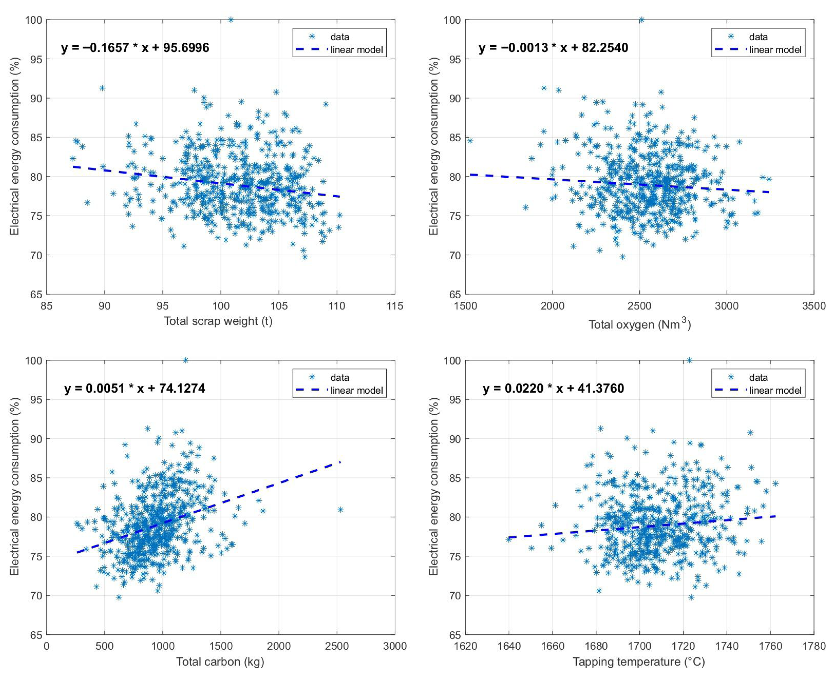
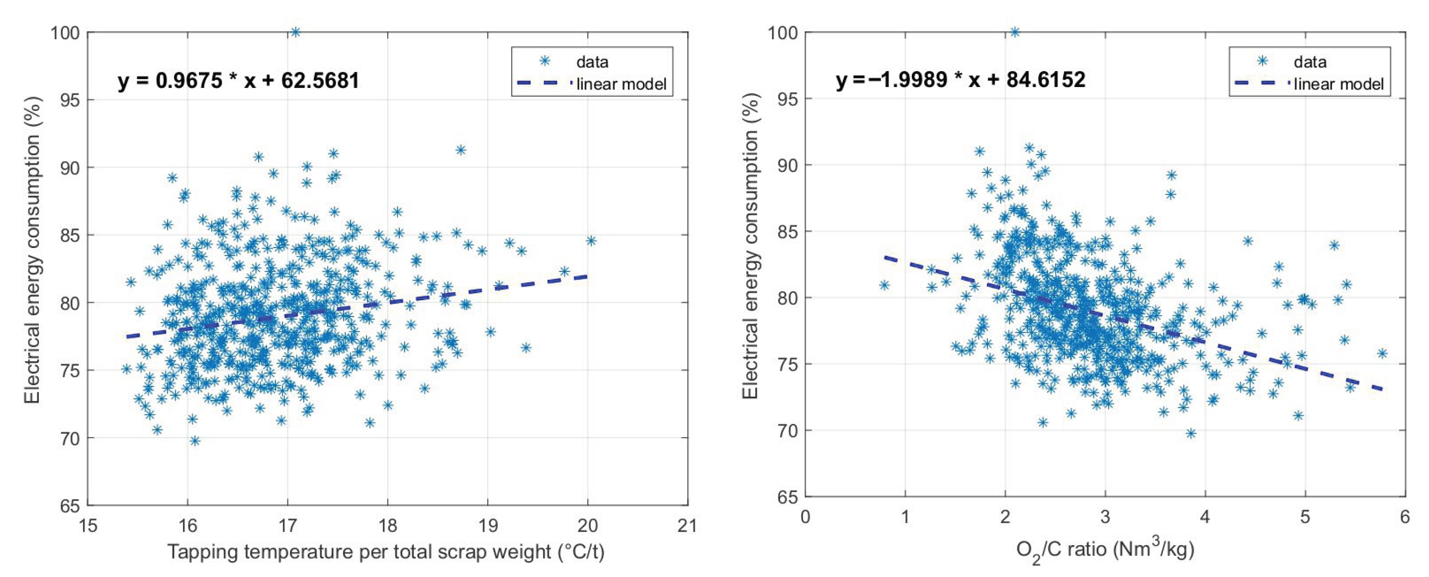
3.1. Results of the Selection of Key Input Variables
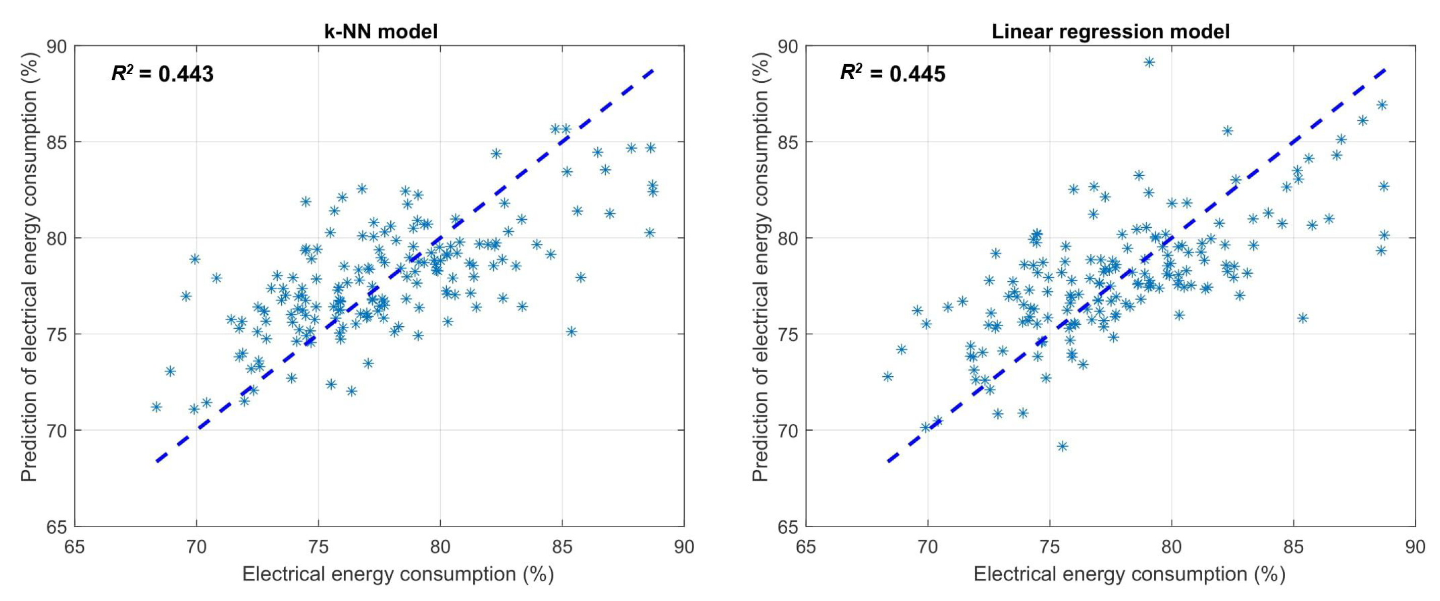
3.2. Analysis of Models for Energy Consumption Prediction
4. Discussion
5. Conclusions
Author Contributions
Funding
Institutional Review Board Statement
Informed Consent Statement
Data Availability Statement
Conflicts of Interest
References
- Toulouevski, Y.N.; Zinurov, I.Y. Modern Steelmaking in Electric Arc Furnaces: History and Development. In Innovation in Electric Arc Furnaces: Scientific Basis for Selection; Springer: Berlin/Heidelberg, Germany, 2013; pp. 1–24. [Google Scholar] [CrossRef]
- Saboohi, Y.; Fathi, A.; Škrjanc, I.; Logar, V. Optimization of the Electric Arc Furnace Process. IEEE Trans. Ind. Electron. 2019, 66, 8030–8039. [Google Scholar] [CrossRef]
- Carlsson, L.S.; Samuelsson, P.B.; Jönsson, P.G. Predicting the Electrical Energy Consumption of Electric Arc Furnaces Using Statistical Modeling. Metals 2019, 9, 959. [Google Scholar] [CrossRef] [Green Version]
- Kovačič, M.; Stopar, K.; Vertnik, R.; Šarler, B. Comprehensive Electric Arc Furnace Electric Energy Consumption Modeling: A Pilot Study. Energies 2019, 12, 2142. [Google Scholar] [CrossRef] [Green Version]
- Sung, Y.; Lee, S.; Han, K.; Koo, J.; Lee, S.; Jang, D.; Oh, C.; Jang, B. Improvement of Energy Efficiency and Productivity in an Electric Arc Furnace through the Modification of Side-Wall Injector Systems. Processes 2020, 8, 1202. [Google Scholar] [CrossRef]
- Echterhof, T. Review on the Use of Alternative Carbon Sources in EAF Steelmaking. Metals 2021, 11, 222. [Google Scholar] [CrossRef]
- Ahmed, W.; Moazzam, M.; Sarkar, B.; Ur Rehman, S. Synergic Effect of Reworking for Imperfect Quality Items with the Integration of Multi-Period Delay-in-Payment and Partial Backordering in Global Supply Chains. Engineering 2021, 7, 260–271. [Google Scholar] [CrossRef]
- Mahapatra, A.S.; N Soni, H.; Mahapatra, M.S.; Sarkar, B.; Majumder, S. A Continuous Review Production-Inventory System with a Variable Preparation Time in a Fuzzy Random Environment. Mathematics 2021, 9, 747. [Google Scholar] [CrossRef]
- Bhuniya, S.; Pareek, S.; Sarkar, B. A supply chain model with service level constraints and strategies under uncertainty. Alex. Eng. J. 2021, 60, 6035–6052. [Google Scholar] [CrossRef]
- Sarkar, B.; Mridha, B.; Pareek, S. A sustainable smart multi-type biofuel manufacturing with the optimum energy utilization under flexible production. J. Clean. Prod. 2022, 332, 129869. [Google Scholar] [CrossRef]
- Yadav, D.; Kumari, R.; Kumar, N.; Sarkar, B. Reduction of waste and carbon emission through the selection of items with cross-price elasticity of demand to form a sustainable supply chain with preservation technology. J. Clean. Prod. 2021, 297, 126298. [Google Scholar] [CrossRef]
- Carlsson, L.S.; Samuelsson, P.B.; Jönsson, P.G. Using Statistical Modeling to Predict the Electrical Energy Consumption of an Electric Arc Furnace Producing Stainless Steel. Metals 2020, 10, 36. [Google Scholar] [CrossRef] [Green Version]
- Logar, V.; Fathi, A.; Škrjanc, I. A Computational Model for Heat Transfer Coefficient Estimation in Electric Arc Furnace. Steel Res. Int. 2016, 87, 330–338. [Google Scholar] [CrossRef]
- Meier, T.; Logar, V.; Echterhof, T.; Škrjanc, I.; Pfeifer, H. Modelling and Simulation of the Melting Process in Electric Arc Furnaces—Influence of Numerical Solution Methods. Steel Res. Int. 2016, 87, 581–588. [Google Scholar] [CrossRef]
- Núñez, A.; De Schutter, B.; Sáez, D.; Škrjanc, I. Hybrid-fuzzy modeling and identification. Appl. Soft Comput. 2014, 17, 67–78. [Google Scholar] [CrossRef]
- Dovžan, D.; Logar, V.; Škrjanc, I. Implementation of an Evolving Fuzzy Model (eFuMo) in a Monitoring System for a Waste-Water Treatment Process. IEEE Trans. Fuzzy Syst. 2015, 23, 1761–1776. [Google Scholar] [CrossRef]
- Škrjanc, I.; Iglesias, J.A.; Sanchis, A.; Leite, D.; Lughofer, E.; Gomide, F. Evolving fuzzy and neuro-fuzzy approaches in clustering, regression, identification, and classification: A Survey. Inf. Sci. 2019, 490, 344–368. [Google Scholar] [CrossRef]
- Fathi, A.; Saboohi, Y.; Škrjanc, I.; Logar, V. Comprehensive Electric Arc Furnace Model for Simulation Purposes and Model-Based Control. Steel Res. Int. 2017, 88, 1600083. [Google Scholar] [CrossRef]
- Hay, T.; Visuri, V.V.; Aula, M.; Echterhof, T. A Review of Mathematical Process Models for the Electric Arc Furnace Process. Steel Res. Int. 2021, 92, 2000395. [Google Scholar] [CrossRef]
- Lee, B.; Sohn, I. Review of Innovative Energy Savings Technology for the Electric Arc Furnace. JOM 2014, 66, 1581–1594. [Google Scholar] [CrossRef]
- Barati, M.; Esfahani, S.; Utigard, T. Energy recovery from high temperature slags. Energy 2011, 36, 5440–5449. [Google Scholar] [CrossRef]
- Lee, B.; Ryu, J.W.; Sohn, I. Effect of Hot Metal Utilization on the Steelmaking Process Parameters in the Electric Arc Furnace. Steel Res. Int. 2015, 86, 302–309. [Google Scholar] [CrossRef]
- Kirschen, M.; Risonarta, V.; Pfeifer, H. Energy efficiency and the influence of gas burners to the energy related carbon dioxide emissions of electric arc furnaces in steel industry. Energy 2009, 34, 1065–1072. [Google Scholar] [CrossRef]
- Bisio, G.; Rubatto, G.; Martini, R. Heat transfer, energy saving and pollution control in UHP electric-arc furnaces. Energy 2000, 25, 1047–1066. [Google Scholar] [CrossRef]
- Meier, T.; Hay, T.; Echterhof, T.; Pfeifer, H.; Rekersdrees, T.; Schlinge, L.; Elsabagh, S.; Schliephake, H. Process Modeling and Simulation of Biochar Usage in an Electric Arc Furnace as a Substitute for Fossil Coal. Steel Res. Int. 2017, 88, 1600458. [Google Scholar] [CrossRef]
- Gandt, K.; Meier, T.; Echterhof, T.; Pfeifer, H. Heat recovery from EAF off-gas for steam generation: Analytical exergy study of a sample EAF batch. Ironmak. Steelmak. 2016, 43, 581–587. [Google Scholar] [CrossRef]
- Glavan, M.; Gradišar, D.; Atanasijević-Kunc, M.; Strmčnik, S.; Mušič, G. Input variable selection for model-based production control and optimisation. Int. J. Adv. Manuf. Technol. 2013, 68, 2743–2759. [Google Scholar] [CrossRef]
- Van De Wal, M.; De Jager, B. Review of methods for input/output selection. Automatica 2001, 37, 487–510. [Google Scholar] [CrossRef] [Green Version]
- May, R.; Dandy, G.; Maier, H. Review of Input Variable Selection Methods for Artificial Neural Networks. In Artificial Neural Networks-Methodological Advances and Biomedical Applications; BoD—Books on Demand: Norderstedt, Germany, 2011. [Google Scholar]
- Li, K.; Peng, J.X. Neural input selection-A fast model-based approach. Neurocomputing 2007, 70, 762–769. [Google Scholar] [CrossRef]
- Breiman, L. Better subset regression using the nonnegative garrote. Technometrics 1995, 37, 373–384. [Google Scholar] [CrossRef]
- Chong, I.G.; Jun, C.H. Performance of some variable selection methods when multicollinearity is present. Chemom. Intell. Lab. Syst. 2005, 78, 103–112. [Google Scholar] [CrossRef]
- Székely, G.J.; Rizzo, M.L.; Bakirov, N.K. Measuring and testing dependence by correlation of distances. Ann. Stat. 2007, 35, 2769–2794. [Google Scholar] [CrossRef]
- Tibshirani, R. Regression Shrinkage and Selection via the Lasso. J. R. Stat. Soc. 1996, 58, 267–288. [Google Scholar] [CrossRef]
- Freedman, D. Statistical Models: Theory and Practice; Cambridge University Press: Cambridge, UK, 2009. [Google Scholar]
- Montgomery, D.C.; Peck, E.A.; Vining, G.G. Introduction to Linear Regression Analysis; John Wiley & Sons: Hoboken, NJ, USA, 2012. [Google Scholar]
- Friedman, J.H.; Bentley, J.L.; Finkel, R.A. An Algorithm for Finding Best Matches in Logarithmic Expected Time. ACM Trans. Math. Softw. 1977, 3, 209–226. [Google Scholar] [CrossRef]
- Chen, G.H.; Shah, D. Explaining the Success of Nearest Neighbor Methods in Prediction. Found. Trends Mach. Learn. 2018, 10, 1–250. [Google Scholar] [CrossRef]
- Takagi, T.; Sugeno, M. Fuzzy identification of systems and its applications to modeling and control. IEEE Trans. Syst. Man Cybern. 1985, SMC-15, 116–132. [Google Scholar] [CrossRef]
- Kennedy, J.; Eberhart, R. Particle swarm optimization. In Proceedings of the ICNN’95-International Conference on Neural Networks, Perth, WA, Australia, 27 November–1 December 1995; Volume 4, pp. 1942–1948. [Google Scholar] [CrossRef]
- Andonovski, G.; Mušič, G.; Blažič, S.; Škrjanc, I. On-line Evolving Cloud-based Model Identification for Production Control. IFAC-PapersOnLine 2016, 49, 79–84. [Google Scholar] [CrossRef]
- Blažič, A.; Škrjanc, I.; Logar, V. Soft sensor of bath temperature in an electric arc furnace based on a data-driven Takagi–Sugeno fuzzy model. Appl. Soft Comput. 2021, 113, 107949. [Google Scholar] [CrossRef]


| Charging | Melting | ||
|---|---|---|---|
| Description | Unit | Description | Unit |
| Total scrap weight | Melting time | ||
| Hotheel start | Delays | ||
| Scrap weight in basket 1 | Temperature | ||
| Scrap weight in basket 2 | Total oxygen | ||
| Scrap weight in basket 3 | Total carbon | ||
| Type of charged scrap | Hotheel end | ||
| Slag weight | |||
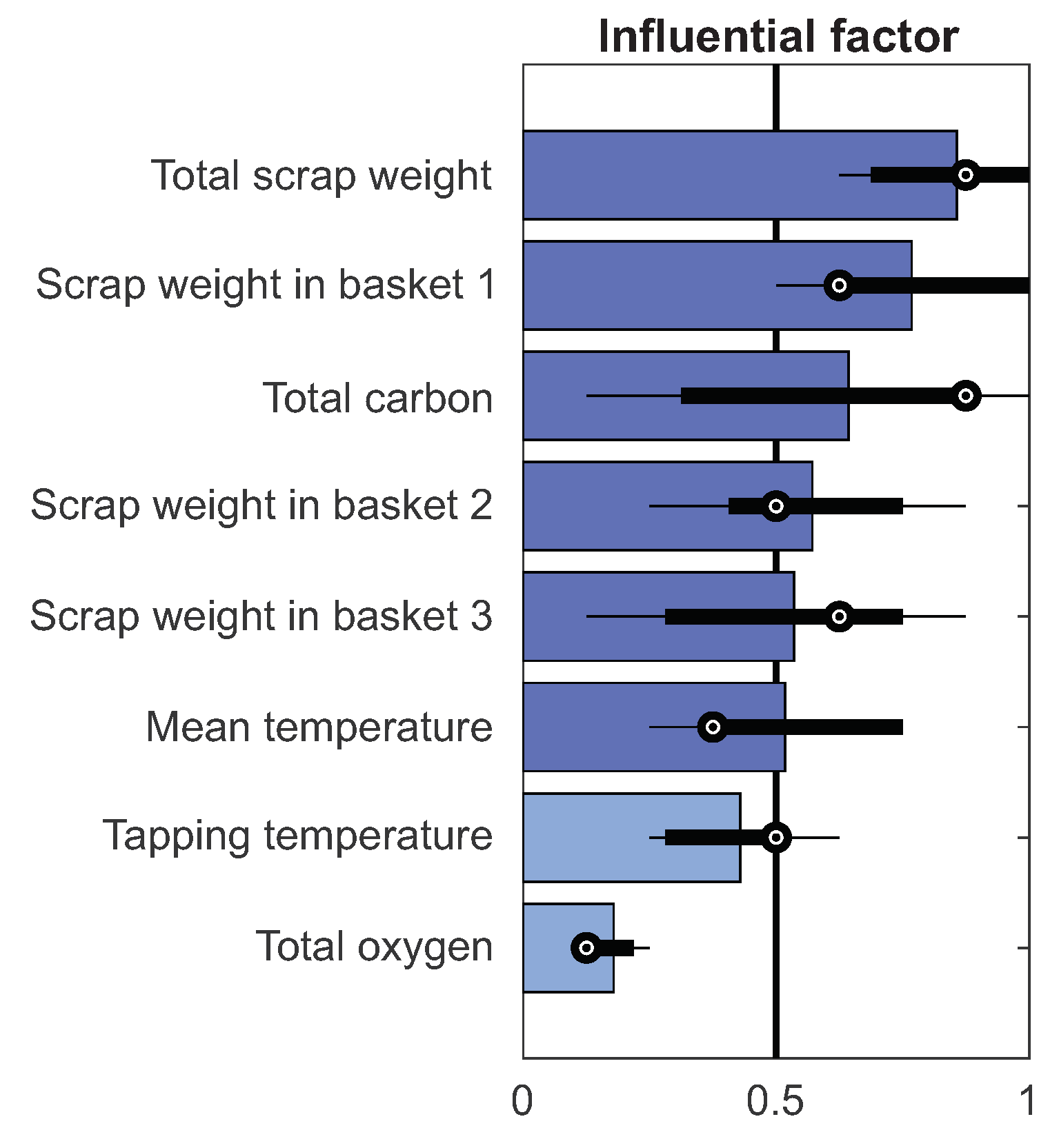
| Variable | Influential Factor |
|---|---|
| Total scrap weight | 0.8571 |
| Scrap weight in basket 1 | 0.7679 |
| Total carbon | 0.6429 |
| Scrap weight in basket 2 | 0.5714 |
| Scrap weight in basket 3 | 0.5357 |
| Mean temperature | 0.5179 |
| Tapping temperature | 0.4286 |
| Total oxygen | 0.1786 |
| Variable | Influential Factor |
|---|---|
| Tapping temperature/total scrap weight | 0.9143 |
| Mean temperature/scrap weight in baskets 1 and 2 | 0.6000 |
| Chemical energy | 0.5143 |
| Total oxygen/total carbon | 0.5143 |
| Scrap weight in baskets 3 | 0.4571 |
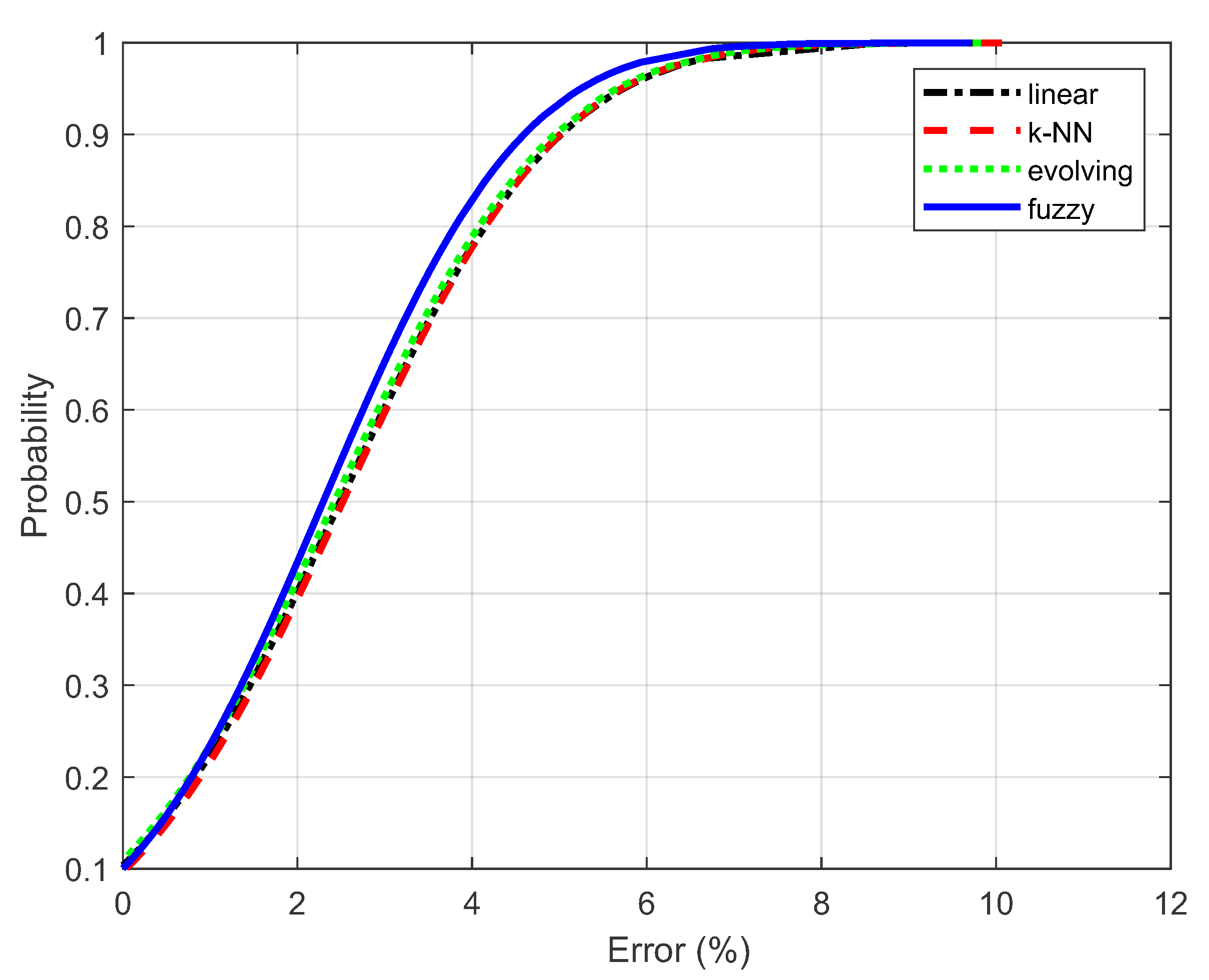
| Method | RMSE (%) | |
|---|---|---|
| k-NN method | 3.177 | 0.443 |
| Linear regression | 3.171 | 0.445 |
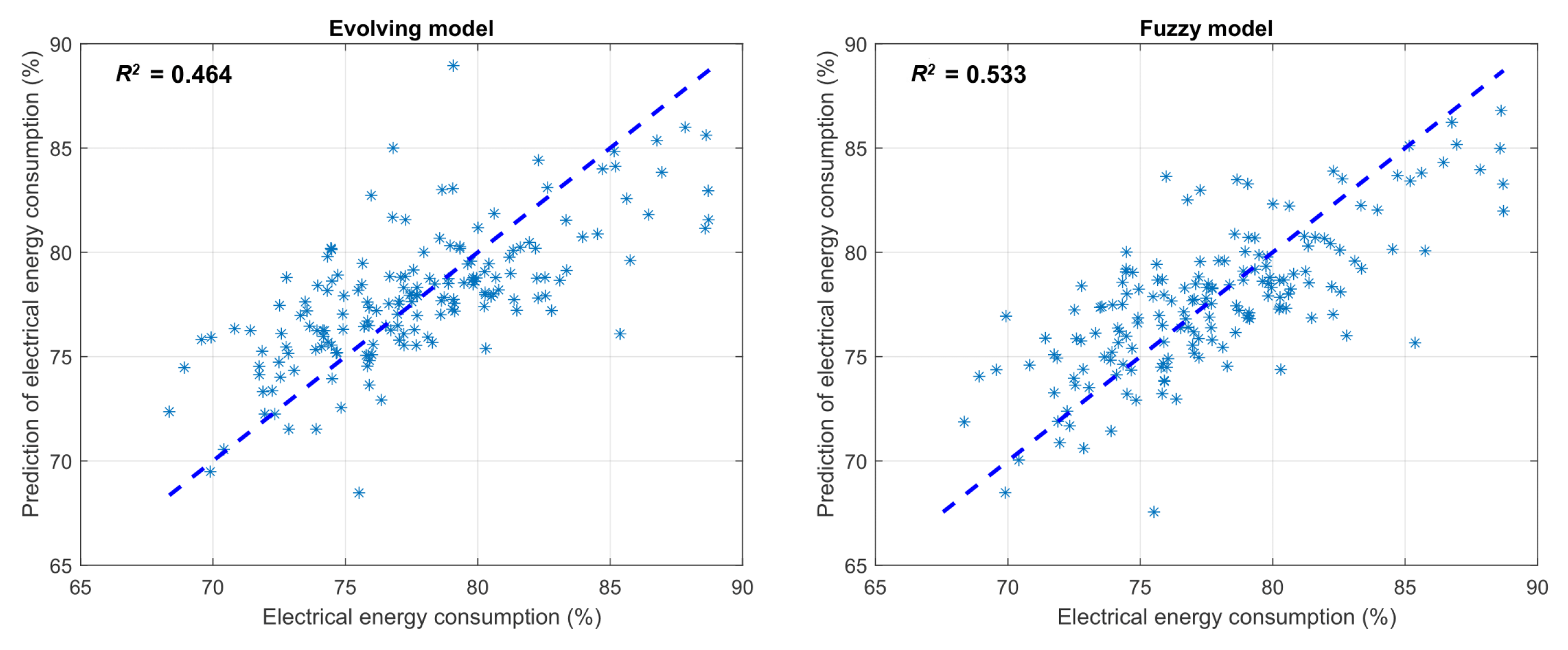
| Evolving model | 3.118 | 0.464 |
| Fuzzy model | 2.910 | 0.533 |
Publisher’s Note: MDPI stays neutral with regard to jurisdictional claims in published maps and institutional affiliations. |
© 2022 by the authors. Licensee MDPI, Basel, Switzerland. This article is an open access article distributed under the terms and conditions of the Creative Commons Attribution (CC BY) license (https://creativecommons.org/licenses/by/4.0/).
Share and Cite
Tomažič, S.; Andonovski, G.; Škrjanc, I.; Logar, V. Data-Driven Modelling and Optimization of Energy Consumption in EAF. Metals 2022, 12, 816. https://doi.org/10.3390/met12050816
Tomažič S, Andonovski G, Škrjanc I, Logar V. Data-Driven Modelling and Optimization of Energy Consumption in EAF. Metals. 2022; 12(5):816. https://doi.org/10.3390/met12050816
Chicago/Turabian StyleTomažič, Simon, Goran Andonovski, Igor Škrjanc, and Vito Logar. 2022. "Data-Driven Modelling and Optimization of Energy Consumption in EAF" Metals 12, no. 5: 816. https://doi.org/10.3390/met12050816