
Recognition of Scratches and Abrasions on Metal Surfaces Using a Classifier Based on a Convolutional Neural Network


Abstract
:1. Introduction
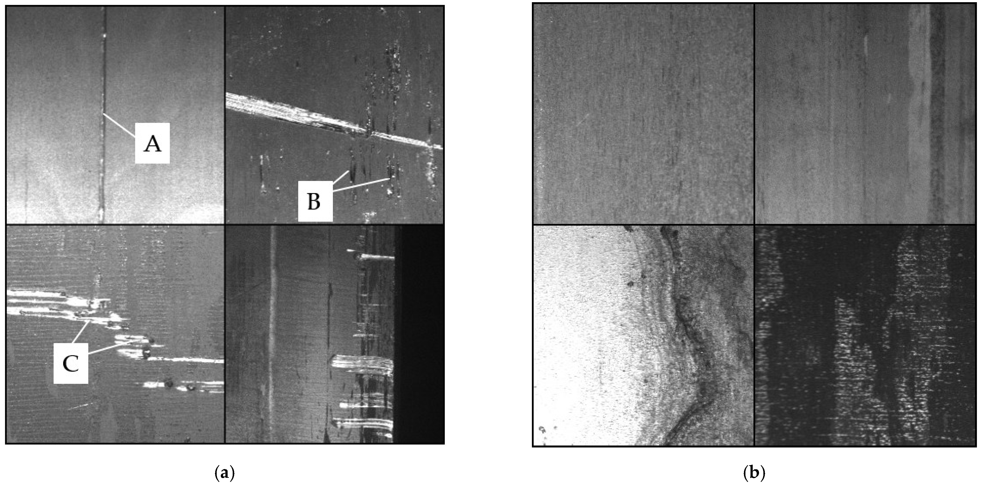
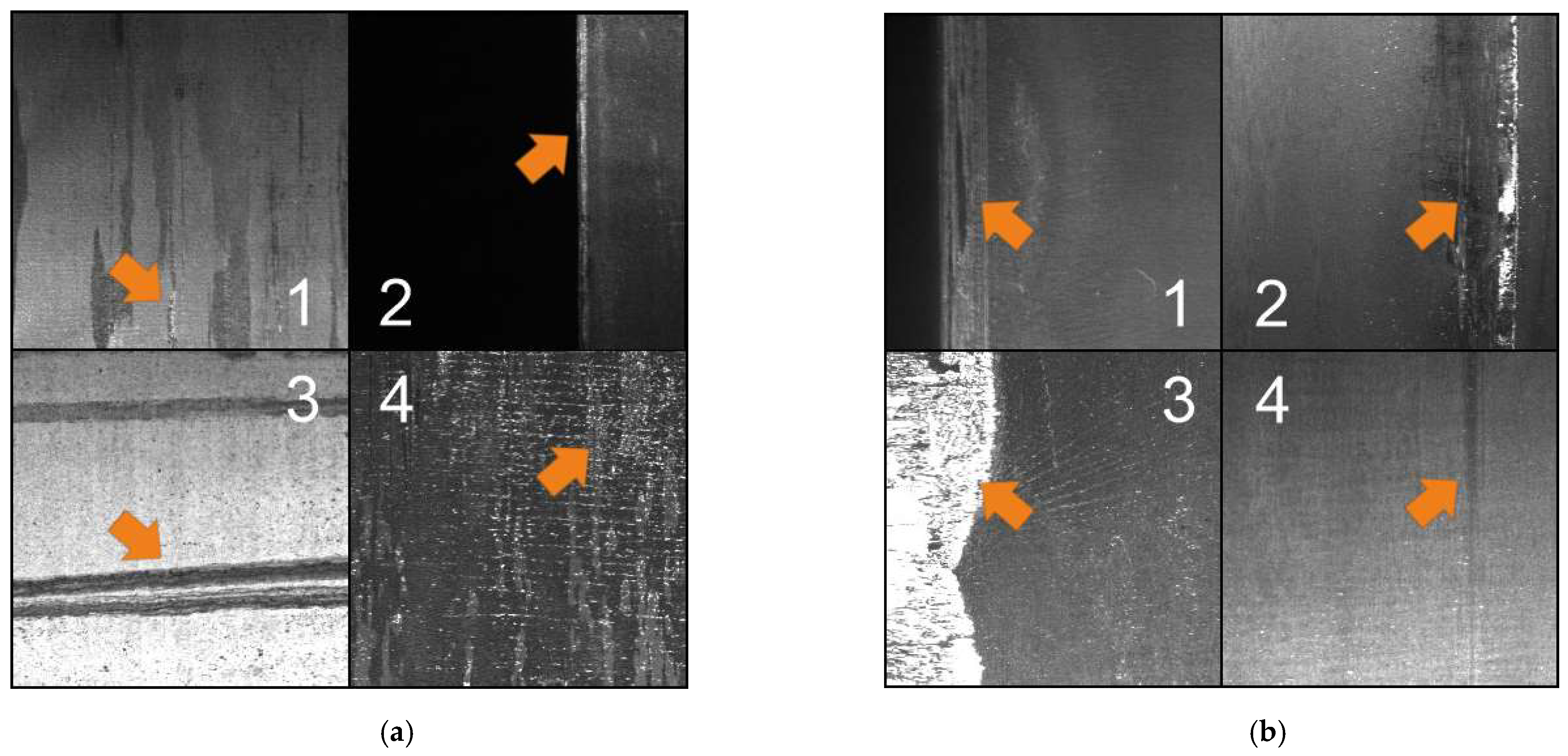
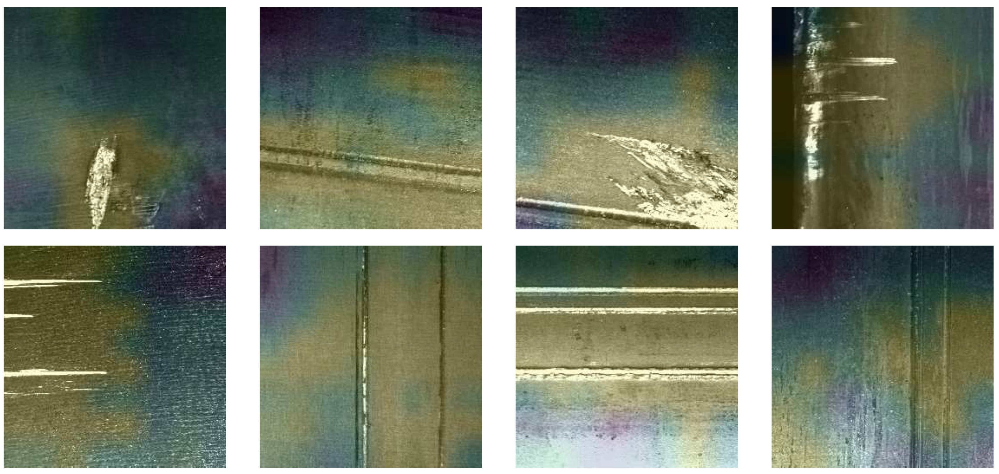
2. Defects
3. Methodology
3.1. Training Dataset
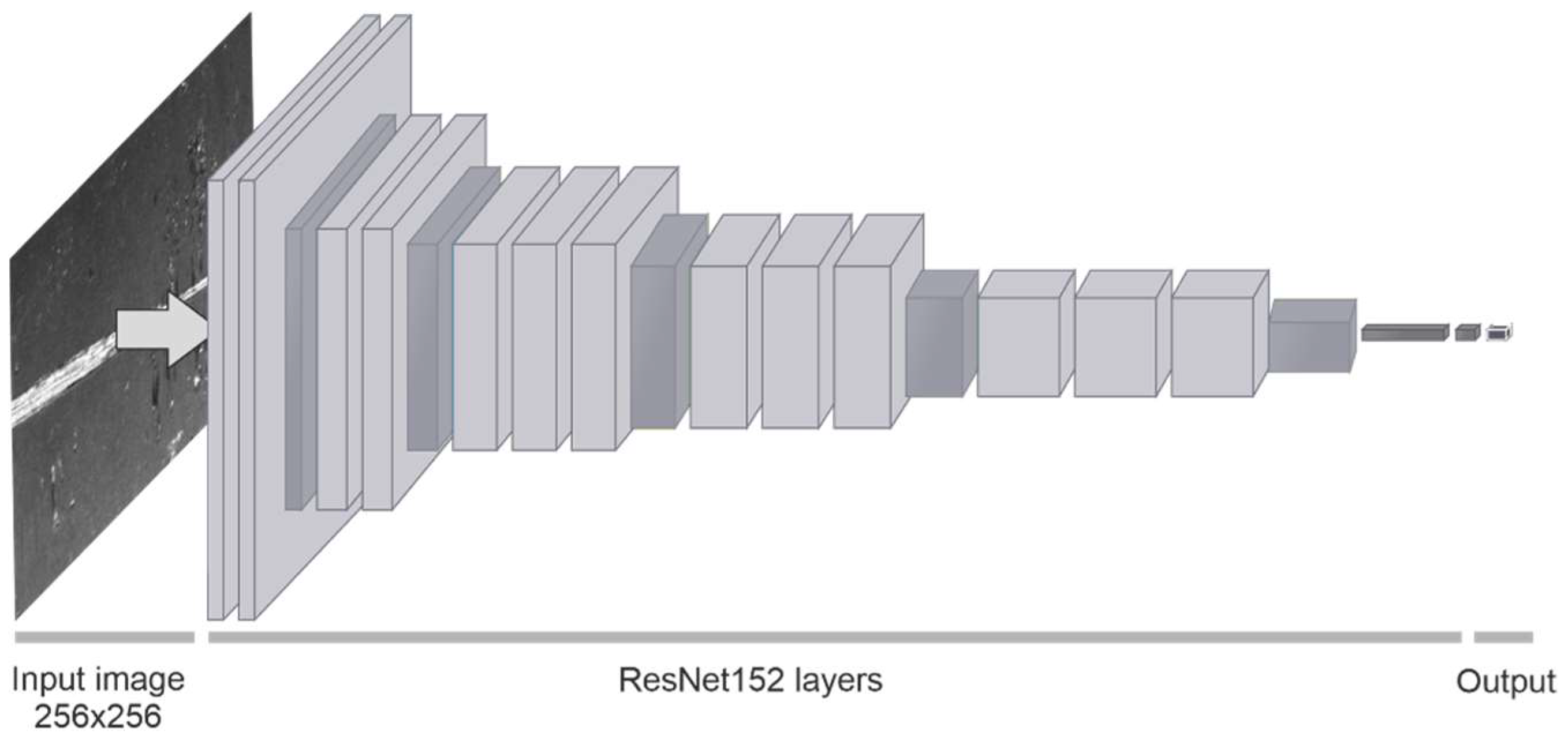
3.2. Neural Network Classifier
- (a)
- Minimal: random crop only,
- (b)
- Basic: random crop and for each crop random flip horizontal, flip vertical or flip both,
- (c)
- Extended: random crop and for each crop random flip horizontal, flip vertical, flip both or random zooming in/out.
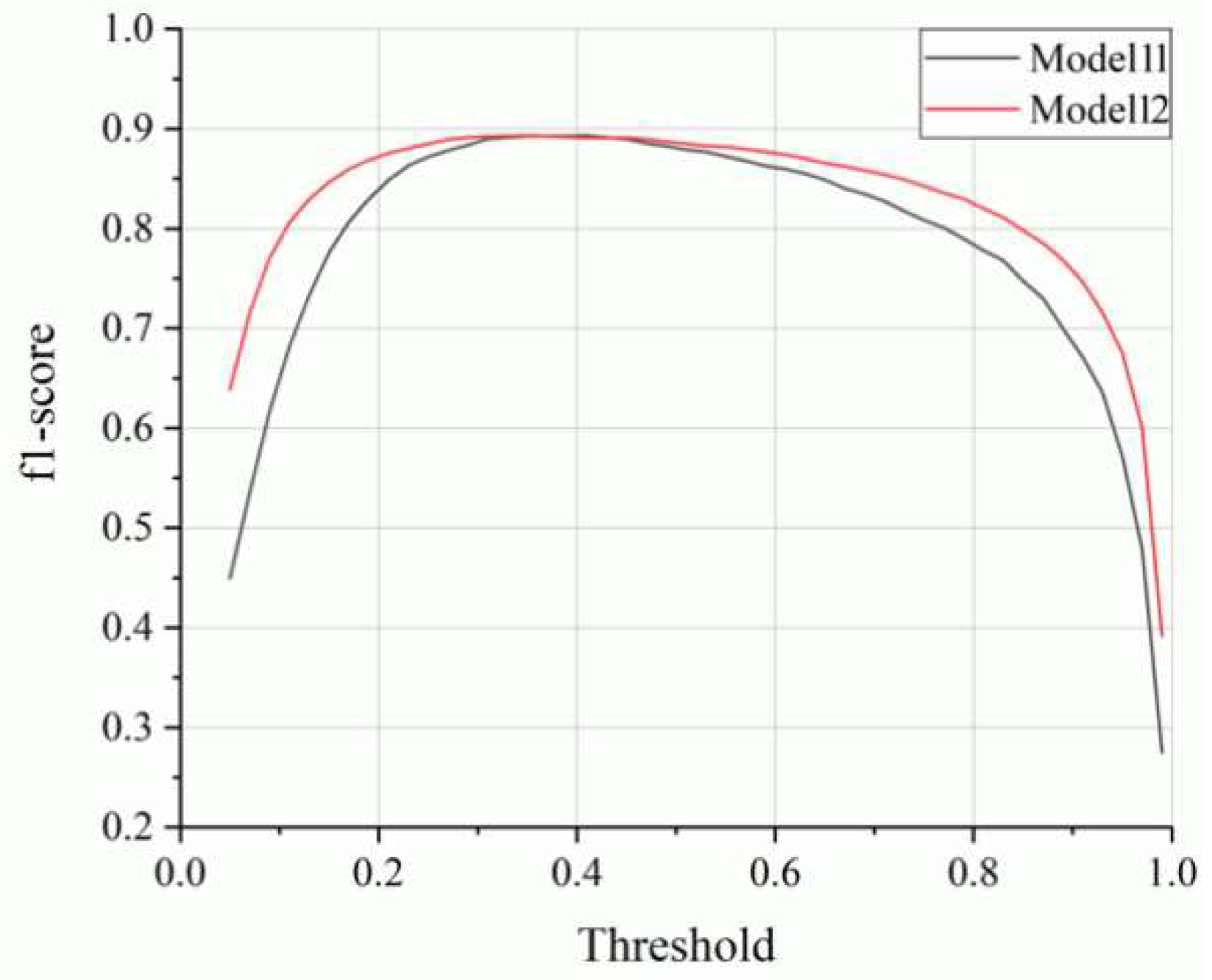
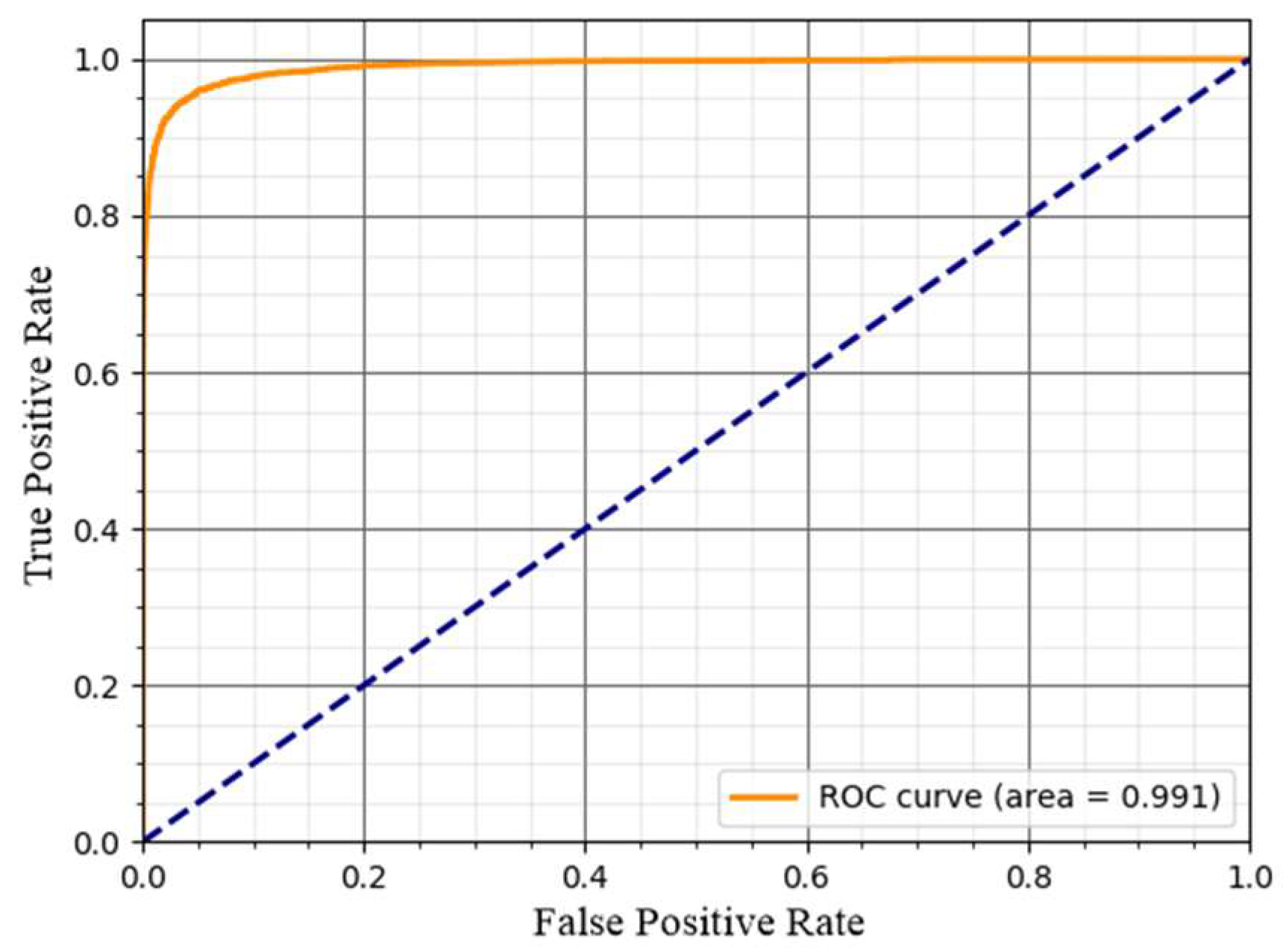
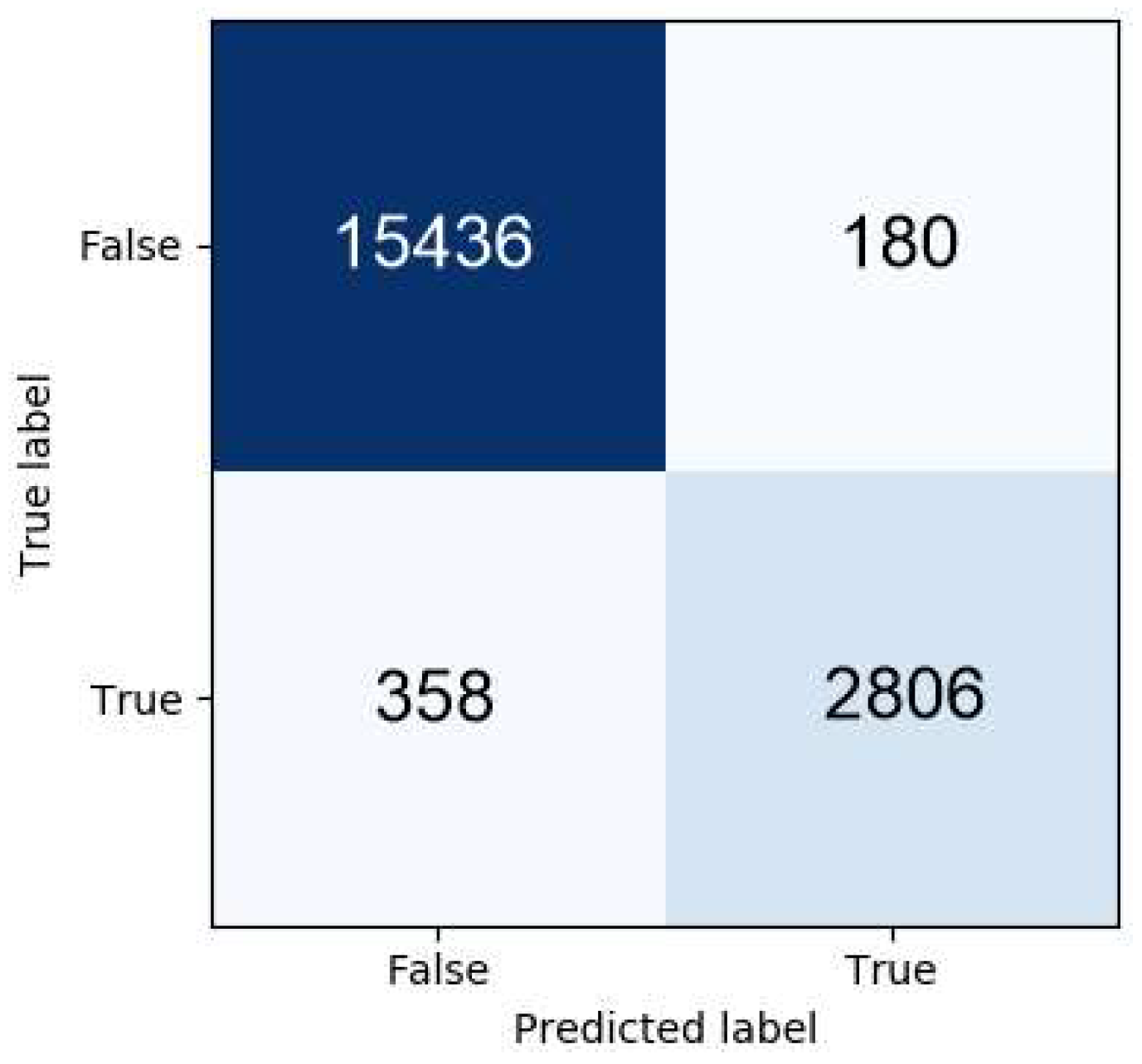
3.3. Model Evaluation Metrics
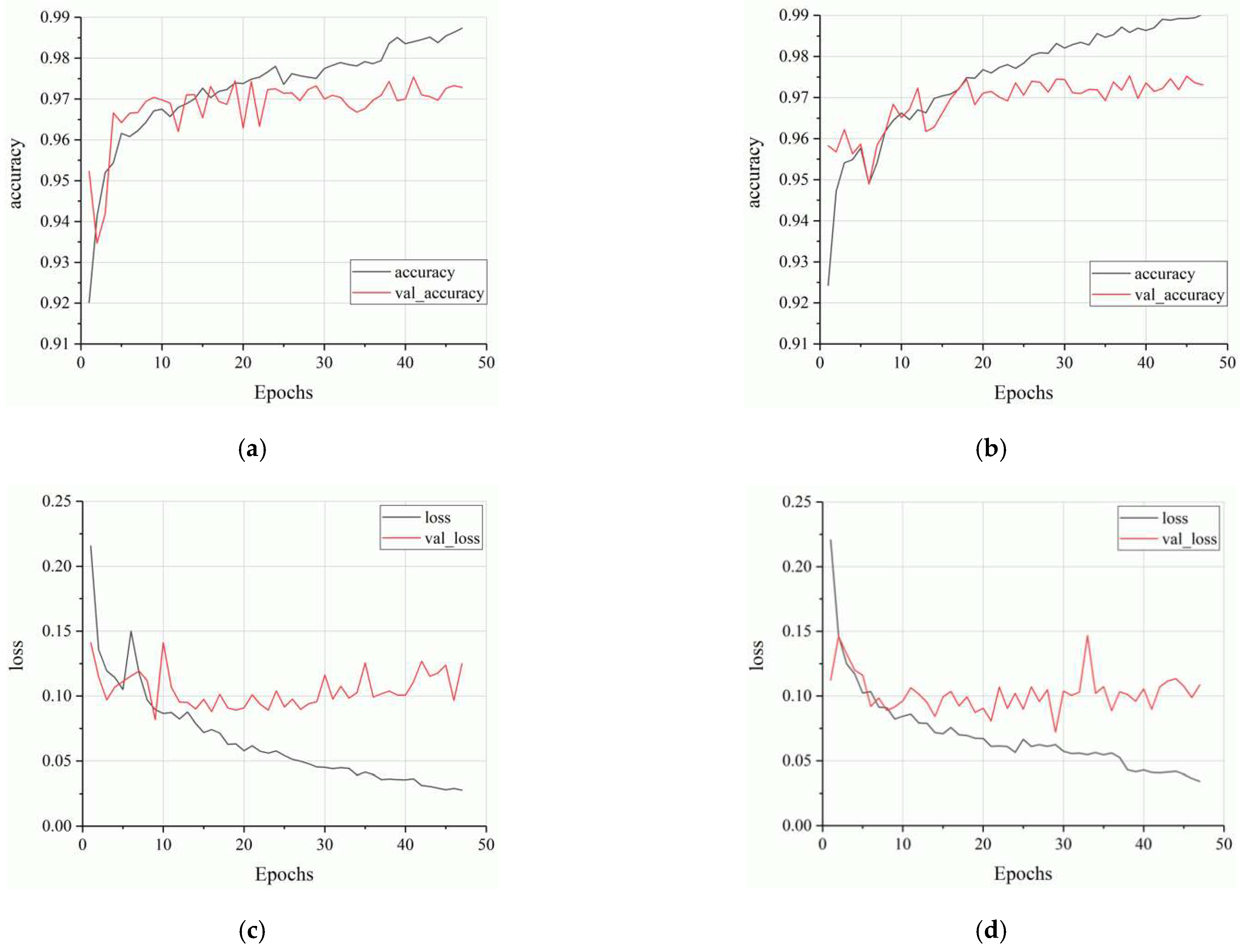
3.4. Models Training and Quality Estimation
3.5. Grad-CAM Class Activation Maps
3.6. Analysis of Images of Any Size
4. Conclusions
Author Contributions
Funding
Data Availability Statement
Conflicts of Interest
References
- Ke, X.; Chaolin, Y. On-line defect detection algorithms for surface inspection of hot rolled strips. In Proceedings of the 2010 International Conference on Mechanic Automation and Control Engineering, Wuhan, China, 26–28 June 2010; pp. 2350–2353. [Google Scholar]
- Becker, D.; Bierwirth, J.; Brachthäuser, N.; Döpper, R.; Thülig, T. Zero-Defect-Strategy in the Cold Rolling Industry. Possibilities and Limitations of Defect Avoidance and Defect Detection in the Production of Cold-Rolled Steel Strip; Fachvereinigung Kaltwalzwerke e.V.; CIELFFA: Düsseldorf, Germany, 2019; p. 16. [Google Scholar]
- Chu, M.-X.; Wang, A.-N.; Gong, R.-F.; Sha, M. Multi-class classification methods of enhanced LS-TWSVM for strip steel surface defects. J. Iron Steel Res. Int. 2014, 21, 174–180. [Google Scholar] [CrossRef]
- Nioi, M.; Celotto, S.; Pinna, C.; Swart, E.; Ghadbeigi, H. Surface defect evolution in hot rolling of high-Si electrical steels. J. Mater. Process. Technol. 2017, 249, 302–312. [Google Scholar] [CrossRef]
- Ren, Q.; Geng, J.; Li, J. Slighter faster R-CNN for real-time detection of steel strip surface defects. In Proceedings of the 2018 Chinese Automation Congress (CAC), Xi’an, China, 30 November–2 December 2018; pp. 2173–2178. [Google Scholar]
- Cong, J.-H.; Yan, Y.-H.; Zhang, H.-A.; Li, J. Real-time surface defects inspection of steel strip based on difference image. In Proceedings of the International Symposium on Photoelectronic Detection and Imaging: Related Technology and Applications 2007, Beijing, China, 9–12 September 2007; Volume 6625, p. 66250W. [Google Scholar]
- Amin, D.; Akhter, S. Deep learning-based defect detection system in steel sheet surfaces. In Proceedings of the 2020 IEEE Region 10 Symposium (TENSYMP), Dhaka, Bangladesh, 5–7 June 2020; pp. 444–448. [Google Scholar]
- Yun, J.P.; Shin, W.C.; Koo, G.; Kim, M.S.; Lee, C.; Lee, S.J. Automated defect inspection system for metal surfaces based on deep learning and data augmentation. J. Manuf. Syst. 2020, 55, 317–324. [Google Scholar] [CrossRef]
- Konovalenko, I.; Maruschak, P.; Brezinová, J.; Viňáš, J.; Brezina, J. Steel surface defect classification using deep residual neural network. Metals 2020, 10, 846. [Google Scholar] [CrossRef]
- Brezinová, J.; Viňáš, J.; Brezina, J.; Guzanová, A.; Maruschak, P. Possibilities for renovation of functional surfaces of backup rolls used during steel making. Metals 2020, 10, 164. [Google Scholar] [CrossRef] [Green Version]
- Yu, H.-L.; Tieu, K.; Lu, C.; Deng, G.-Y.; Liu, X.-H. Occurrence of surface defects on strips during hot rolling process by FEM. Int. J. Adv. Manuf. Technol. 2013, 67, 1161–1170. [Google Scholar] [CrossRef] [Green Version]
- Mikołajczyk, T.; Nowicki, K.; Kłodowski, A.; Pimenov, D. Neural network approach for automatic image analysis of cutting edge wear. Mech. Syst. Signal Process. 2017, 88, 100–110. [Google Scholar] [CrossRef]
- Ferreira, A.; Giraldi, G. Convolutional neural network approaches to granite tiles classification. Expert Syst. Appl. 2017, 84, 1–11. [Google Scholar] [CrossRef]
- Yi, L.; Li, G.; Jiang, M. An end-to-end steel strip surface defects recognition system based on convolutional neural networks. Steel Res. Int. 2017, 88, 87. [Google Scholar] [CrossRef]
- Kim, M.S.; Park, T.; Park, P. Classification of steel surface defect using convolutional neural network with few images. In Proceedings of the 12th Asian Control Conference (ASCC), Kitakyusyu International Conference Center, Fukuoka, Japan, 9–12 June 2019; pp. 1398–1401. [Google Scholar]
- Urbikain, G.; Alvarez, A.; De Lacalle, L.N.L.; Arsuaga, M.; Alonso, M.A.; Veiga, F. A reliable turning process by the early use of a deep simulation model at several manufacturing stages. Machines 2017, 5, 15. [Google Scholar] [CrossRef]
- Bustillo, A.; Urbikain, G.; Perez, J.M.; Pereira, O.M.; de Lacalle, L.N.L. Smart optimization of a friction-drilling process based on boosting ensembles. J. Manuf. Syst. 2018, 48, 108–121. [Google Scholar] [CrossRef]
- Zhao, W.; Chen, F.; Huang, H.; Li, D.; Cheng, W. A new steel defect detection algorithm based on deep learning. Comput. Intell. Neurosci. 2021, 2021. [Google Scholar] [CrossRef]
- Kaggle. Severstal: Steel Defect Detection. Can You Detect and Classify Defects in Steel? 2019. Available online: https://www.kaggle.com/c/severstal-steel-defect-detection (accessed on 27 March 2021).
- Northeastern University. Available online: https://www.kaggle.com/kaustubhdikshit/neu-surface-defect-database (accessed on 27 March 2021).
- He, K.; Zhang, X.; Ren, S.; Sun, J. Deep Residual learning for image recognition. In Proceedings of the 2016 IEEE Conference on Computer Vision and Pattern Recognition (CVPR), Las Vegas, NV, USA, 27–30 June 2016; pp. 770–778. [Google Scholar] [CrossRef] [Green Version]
- Simonyan, K.; Zisserman, A. Very deep convolutional networks for large-scale image recognition. arXiv 2014, arXiv:1409.15561556v6. [Google Scholar]
- Taylor, M.E.; Stone, P. Transfer learning for reinforcement learning domains: A survey. J. Mach. Learn. Res. 2009, 10, 1633–1685. [Google Scholar]
- Khan, S.; Islam, N.; Jan, Z.; Din, I.U.; Rodrigues, J.J.P.C. A novel deep learning based framework for the detection and classification of breast cancer using transfer learning. Pattern Recognit. Lett. 2019, 125, 1–6. [Google Scholar] [CrossRef]
- Maqsood, M.; Nazir, F.; Khan, U.; Aadil, F.; Jamal, H.; Mehmood, I.; Song, O.-Y. Transfer learning assisted classification and detection of Alzheimer’s disease stages using 3D MRI scans. Sensors 2019, 19, 2645. [Google Scholar] [CrossRef] [Green Version]
- Yu, X.; Wu, X.; Luo, C.; Ren, P. Deep learning in remote sensing scene classification: A data augmentation enhanced convolutional neural network framework. GISci. Remote Sens. 2017, 54, 741–758. [Google Scholar] [CrossRef] [Green Version]
- Eyobu, O.S.; Han, D.S. Feature representation and data augmentation for human activity classification based on wearable IMU sensor data using a deep LSTM neural network. Sensors 2018, 18, 2892. [Google Scholar] [CrossRef] [Green Version]
- Han, D.; Liu, Q.; Fan, W. A new image classification method using CNN transfer learning and web data augmentation. Expert Syst. Appl. 2018, 95, 43–56. [Google Scholar] [CrossRef]
- Konovalenko, I.; Maruschak, P.; Prentkovskis, O.; Junevičius, R. Investigation of the rupture surface of the titanium alloy using convolutional neural networks. Materials 2018, 11, 2467. [Google Scholar] [CrossRef] [Green Version]
- Takahashi, R.; Matsubara, T.; Uehara, K. Data augmentation using random image cropping and patching for deep CNNs. IEEE Trans. Circuits Syst. Video Technol. 2020, 30, 2917–2931. [Google Scholar] [CrossRef] [Green Version]
- Lin, T.-Y.; Goyal, P.; Girshick, R.B.; He, K.; Dollar, P. Focal loss for dense object detection. IEEE Trans. Pattern Anal. Mach. Intell. 2020, 42, 318–327. [Google Scholar] [CrossRef] [PubMed] [Green Version]
- Chollet, F. Deep Learning with Python; Manning Publications: Shelter Island, NY, USA, 2017; p. 313. [Google Scholar]
- Wang, S.; Xia, X.; Ye, L.; Yang, B. Automatic detection and classification of steel surface defect using deep convolutional neural networks. Metals 2021, 11, 388. [Google Scholar] [CrossRef]
- Selvaraju, R.R.; Cogswell, M.; Das, A.; Vedantam, R.; Parikh, D.; Batra, D. Grad-CAM: Visual explanations from deep networks via gradient-based localization. Int. J. Comput. Vis. 2020, 128, 336–359. [Google Scholar] [CrossRef] [Green Version]
- Tishchenko, D.A. Development of Control Algorithms, Modes of Preparation and Operation of Work Rolls of the Finishing Group of a Continuous Wide-Strip Hot Rolling Mill to Ensure the Quality of Rolled Products. CSc. (Eng.) Dissertation, JSC, Institute Tsvetmetobrabotka, Moscow, Russia, 2006; p. 160. (In Russian). [Google Scholar]


| Model No | Architecture | Initial Learning Rate | Augmentation |
|---|---|---|---|
| 1 | ResNet50 | 0.01 | a |
| 2 | ResNet50 | 0.01 | b |
| 3 | ResNet50 | 0.01 | c |
| 4 | ResNet50 | 0.001 | a |
| 5 | ResNet50 | 0.001 | b |
| 6 | ResNet50 | 0.001 | c |
| 7 | ResNet152 | 0.01 | a |
| 8 | ResNet152 | 0.01 | b |
| 8 | ResNet152 | 0.01 | c |
| 10 | ResNet152 | 0.001 | a |
| 11 | ResNet152 | 0.001 | b |
| 12 | ResNet152 | 0.001 | c |
| Model No | Accuracy | Precision | Recall | f1 Score |
|---|---|---|---|---|
| 1 | 0.9595 | 0.9894 | 0.7692 | 0.8655 |
| 2 | 0.9654 | 0.9780 | 0.8139 | 0.8885 |
| 3 | 0.9664 | 0.9764 | 0.8212 | 0.8921 |
| 4 | 0.9641 | 0.9826 | 0.8020 | 0.8831 |
| 5 | 0.9674 | 0.9532 | 0.8488 | 0.8980 |
| 6 | 0.96757 | 0.9713 | 0.8328 | 0.8967 |
| 7 | 0.9666 | 0.9608 | 0.8362 | 0.8942 |
| 8 | 0.9662 | 0.9644 | 0.8307 | 0.8926 |
| 9 | 0.9686 | 0.9685 | 0.8419 | 0.9008 |
| 10 | 0.9647 | 0.9134 | 0.8733 | 0.8929 |
| 11 | 0.9682 | 0.9381 | 0.8696 | 0.9025 |
| 12 | 0.9714 | 0.9397 | 0.8869 | 0.9125 |
Publisher’s Note: MDPI stays neutral with regard to jurisdictional claims in published maps and institutional affiliations. |
© 2021 by the authors. Licensee MDPI, Basel, Switzerland. This article is an open access article distributed under the terms and conditions of the Creative Commons Attribution (CC BY) license (http://creativecommons.org/licenses/by/4.0/).
Share and Cite
Konovalenko, I.; Maruschak, P.; Brevus, V.; Prentkovskis, O. Recognition of Scratches and Abrasions on Metal Surfaces Using a Classifier Based on a Convolutional Neural Network. Metals 2021, 11, 549. https://doi.org/10.3390/met11040549
Konovalenko I, Maruschak P, Brevus V, Prentkovskis O. Recognition of Scratches and Abrasions on Metal Surfaces Using a Classifier Based on a Convolutional Neural Network. Metals. 2021; 11(4):549. https://doi.org/10.3390/met11040549
Chicago/Turabian StyleKonovalenko, Ihor, Pavlo Maruschak, Vitaly Brevus, and Olegas Prentkovskis. 2021. "Recognition of Scratches and Abrasions on Metal Surfaces Using a Classifier Based on a Convolutional Neural Network" Metals 11, no. 4: 549. https://doi.org/10.3390/met11040549