1. Introduction
Modelling the friction behavior of wet multi-plate clutches is difficult, whereas at the same time, the friction behavior is the key parameter defining thermal loads and comfort characteristics [
1]. However, simulation of the thermal behavior of wet clutches is essential during the design phase as thermal loads determine lifetime and performance [
2,
3]. In addition to high quality modeling approaches, reliable input data, especially for Coefficient of Friction (CoF), which defines the energy input, is needed for the calculation of the thermal behavior [
4]. Experimental research on the friction behavior of wet clutches shows various influencing factors, e.g., lubricant, material and applied load (a.o., [
5,
6,
7,
8]). Due to the lack of hands-on applicable friction models, energy input is often modeled with constant CoF, friction maps (e.g., [
9]) or models lacking any possible physical interpretation (e.g., [
10]). The development of state-of-the-art friction models is based on physical modelling or curve fitting methods. Sophisticated physical modelling approaches exist in the case of elastohydrodynamic lubrication (EHL) based on Reynolds linear elasticity, solid mechanics and load balance equations [
11]. In general, the deviations between numerical predictions and experiments of CoF are, for low entrainment speeds during ball on disc tests, less than 10% [
11]. However, the application of EHL methods to wet clutches is not appropriate due to low contact pressure and very small hydrodynamic film buildup [
12]. Nevertheless, there are physical models from the application of dynamic pressure lubrication theory and Hertz contact theory, which make it possible to estimate the CoF in wet clutches and help to understand the friction mechanisms [
13,
14]. However, their practical relevance is limited due to the assumptions and simplifications made during model derivation.
In addition to these physical approaches, there are many empirical models, parametrized by curve fitting with measurement data. The models consist of linear/quadratic (a.o., [
15]), logarithmic (a.o., [
15,
16]), exponential (a.o., [
17]), hyperbolic (a.o., [
18]) or combinations of these terms (a.o., [
15,
19]). Another approach is fitting of the Stribeck curve to measurement data (a.o., [
20,
21,
22]. All these models have the sliding velocity (or rotational speed) as an input parameter in common, sometimes extended by clutch pressure and contact temperature [
13,
19,
21]. Logarithmic approaches are motivated by the logarithmic dependence of shear stress of the organic friction modifier boundary films [
12], but need special treatment for zero sliding velocity. Stribeck-curve models separate the friction behavior in the static and kinetic friction coefficient and try to combine curve fitting methods with the possibility of physical interpretation. Most of these empirical models concentrate on reproducing the friction behavior of a single friction system. Furthermore, sliding velocity is often considered to be the only variable model input parameter.
Recent research also applies data mining [
23] and machine learning [
24] techniques to the torque transfer behavior of wet clutches. The data mining approach analyses friction behavior and states the main influences on the CoF of the studied tribological system in descending order, such as clutch pressure, friction surface temperature, feeding lubricant temperature and differential speed. The authors state their approach as superior to classical one factor at a time and designed experiment approaches but do not rate the high effort of experiments in applying their method [
23]. The machine learning approach focuses on non-linear torque transfer function representing the whole clutch system and is therefore not a contribution for modelling the CoF [
24].
In addition, there is ongoing research on the design of experimental test methods for the characterization of the friction behavior of new friction systems A reduction in test duration is focused by most test methods as it directly reduces costs and effort. Screening tests offer the possibility of evaluating the friction behavior of new tribological systems within hours under various load conditions and of differentiating the performance of different systems (a.o., [
8,
25,
26]). However, it requires a high level of experience to meet application relevant conditions.
In addition to classical approaches, the application of the method of designed experiments and ensemble techniques facilitates the application of statistical methods (e.g., ANOVA) and derivation of regression models during data evaluation (e.g., [
27,
28]). These methods have been successfully applied to examine the effects of non-uniform torque [
29], to develop regression models for describing the vibration-reducing effect of wet clutch systems [
30] and to build regression models of clutch engagement [
31].
The literature review shows work in progress in identifying appropriate friction models of wet clutches. However, most models are tested with one system only and it is therefore not clear if the results are applicable to different clutch systems. Furthermore, there is a lack of published data on the experimental setup for deriving these models.
This contribution describes a new approach for the identification and evaluation of friction models, with focus on facilitating and improving the estimation of CoF as an input parameter for simulation models such as thermal calculations. The experimental investigation is based on designed experiments to enable the application of analysis of variance (ANOVA) and stepwise regression. We develop easy-to-use linear friction models of three different clutch designs from serial production and validate the results with measurement data. We discuss the quality and transferability of the linear friction models. Furthermore, the applied methods allow the determination and characterization of significant influencing parameters on the CoF of the investigated friction systems.
2. Experimental Setup and Data Collection
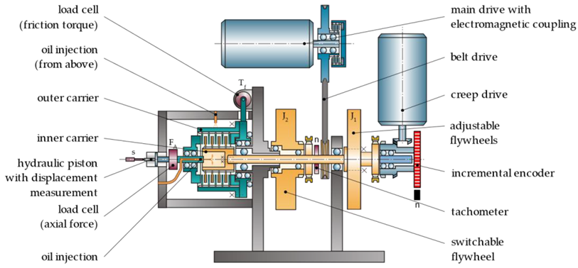
The experimental investigations are carried out on a wet brake component test rig ZF/FZG KLP-260. The description of the test rig is according to [
26,
32]. The test rig operates in brake mode with a fixed outer carrier and rotating inner carrier, as pictured in
Figure 1.
The test rig enables mounting of a complete clutch pack with corresponding carriers. Inner plates are placed on the inner carrier which is connected to the inner shaft and connected to the fly wheels (J1, J2). Friction work of the clutch can be adjusted through variable configurations of the fly wheels J1 and by engaging inertia J2.
Axial force is applied to the plates by a force controlled hydraulic piston. Friction torque is measured at the outer carrier. Cooling oil can be supplied centrally in the inner carrier, externally from the top of the housing or by oil sump. The oil flow rate and the thermostat-controlled feeding temperature can be adjusted over a wide range. For brake engagement tests, the main shaft with inner carrier and fly wheels is accelerated by the speed-controlled main drive up to a defined speed n. During engagement, the main drive and the inner shaft are decoupled through an electromagnetic coupling. Under creeping conditions and in non-steady and constant slip mode a defined axial force is applied to the clutch plates. Either creep or main drive then accelerates the inner shaft up to a defined slip speed. The rotational speed in low-speed creep and slip modes is measured with high resolution by an incremental encoder.
Table 1 shows the technical data of the test rig.
The measurement accuracy of the test rig is determined by applying the rules of the Guide to the Expression of Uncertainty in Measurement (GUM) [
24] and DIN EN ISO 14253-2 [
25] to the ZF/FZG KLP-260 test rig as published in [
33,
34].
Table 2 summarizes the measurement accuracy for the FZG/ZF KLP-260 test rig.
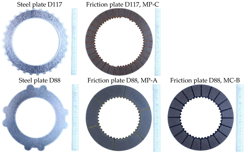
For the experimental studies, we use steel (outer) and friction (inner) plates from the serial production of automotive applications with organic friction linings (paper MP/carbon MC). Three tribological systems are investigated. We vary the clutch size, characterized by the mean diameter of the clutches (88/117 mm), friction lining material (MP-A/MP-C/MC-B) and lubricant (L-103/L-201/L-205). All friction plates have a multi-segmented groove pattern. One clutch package consists of five steel plates and four friction plates. Thus, there are eight friction interfaces (z = 8). The nominal clearance between each friction plate and steel plate is 0.20 mm.
Figure 2 pictures the steel and friction plates.
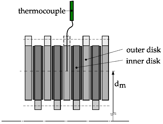
We measure mass temperatures in the center steel plate at several evenly spaced circumferential positions with thermocouples (NiCrNi Type K Class 1, Ø 0.25/0.5 mm, response time approximately 10/30 ms calculated according to [
35], as sketched in
Figure 3. Therefore, we apply a high-density polysynthetic silver thermal compound to the thermocouples and place them in a circumferential drill hole (Ø 0.3/0.6 mm) approximately down to the mean diameter (d
m) positioned in the midplane of the respective steel plate. To determine the mass temperature of the steel plate, the signals of the thermocouples distributed around the circumference are averaged.
Table 3 summarizes the technical data obtained from the lubricants’ data sheets.
Table 4 summarizes the friction systems consisting of the clutch packages and the corresponding lubricants.
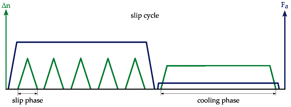
During the experiment, the clutches operate in a non-steady slip condition.
Figure 4 shows an example of the course of the axial force (F
a) and differential speed (Δn) during non-steady slip. The clutch is closed by applying the axial force. The following multiple slip phases are characterized by acceleration of the clutch to a maximum differential speed Δn and immediately after reaching this differential speed, it is decelerated again with the same gradient to the initial speed of zero. The slip phases are repeated for a defined number of times (in this study 5). After the last slip phase, the clutch is briefly released. A cooling phase follows to allow the clutch components to cool down. This is defined by a fixed differential speed of Δn = 20 rpm and an axial force of F
a = 100 N, which is maintained until the middle steel plate reaches a steady temperature. The low axial force ensures distribution of the cooling oil in the grooves around the circumference of the clutch.
As suggested in [
36], all designed experiments are performed after 100 running-in collectives in non-steady slip to eliminate non-linear effects occurring in the first engagements. The running-in load stages are summarized in
Table 5. A running-in collective consists of the six load stages (LS) running in the order E1 … E6, whereas a cooling phase (EC) is held after each load stage for 20 s. The specific oil flow rate is 1 mm³/mm²s and the oil injection temperature is 80 °C during running-in collectives.
The designed test plan is based on a randomized two-level, four-factor, full-factorial design. We vary the oil injection temperature, feeding oil flow rate, clutch pressure and differential speed on two levels, thus resulting in 16 load stages in non-steady slip operation. Oil is supplied centrally during all runs. The measurements of systems D117/MP-C and D88/MC-B are repeated once, resulting in 32 runs in total. We use blocking to search for significant differences between the first and second run.
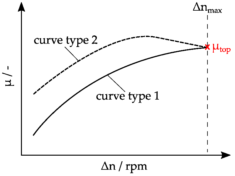
The measured value is µ
top which represents the value of the CoF at maximum differential speed.
Figure 5 shows an explanation for the measured value for two types of friction characteristics (course of CoF over sliding velocity) leading to equivalent values of µ
top. We evaluate µ
top of the last slip phase of each slip cycle. We use the mean average of µ
top from the last five slip cycles of each load stage as an input parameter for our linear friction models. The values µ
top are used as output values for the model.
Each slip cycle is repeated 10 times with the same factor settings (load stages). The duration of the cooling phases at the end of each slip cycle is varied such that the temperature in the center steel plate at the beginning of the next slip cycle is nearly constant. The oil is supplied centrally to the inner carrier. The application of the full-factorial design defines 16 load stages as summarized in
Table 6. The sequence of load stages is randomized, except for oil injection temperature. All specific values are normalized by gross friction surface area. The load stages cover typical working conditions of the clutch in practical applications. In addition to the load stages mentioned in
Table 6, the steel plate temperature (Symbol E) is measured as covariate. All mentioned factors and the covariate are possible input variables for the models.
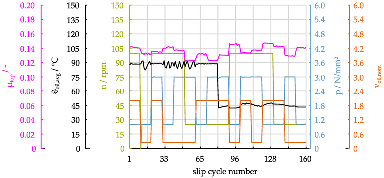
Figure 6 shows the measurement of the varied factors (oil injection temperature, nominal feeding oil flow rate, clutch pressure, maximum differential speed) and the measured variable (µ
top) of each slip cycle of system D117/MP-C during the first run of the full-factorial test. Each block consists of 160 data samples, respectively slip cycles.
3. Methods
To analyze the gathered data, we apply and implement two methods for statistical analysis in MatLab (The MathWorks, Inc., Natick, MA, USA). The scope is the evaluation of the impact of the main effects and their interactions on the characteristic value
.
This is the basis for identifying statistically significant factors and an appropriate linear friction model as a combination of factors. A model consisting of a constant n
f main effects and all their two-fold interactions according to [
27] can be described as
Here, the model constants c and the input variables x give an approximation for the output variable y with the model deviation ε. This deviation should be small for an appropriate model. The first sum describes the main effects. The combined sum describes the two-fold interaction terms.
The first method is the analysis of variance (ANOVA), which establishes the null hypothesis that all factor groups have the same mean value. The variability in the dataset is described by the total sum of squares (TSS), which then gets split into two components. The variability between the groups (Sum of Squares Between; SSB) describes the effect of the corresponding factor, while the variability within the groups (Sum of Squares Within; SSW) can be interpreted as measurement noise or model error. For every available factor, the F-value is defined as the ratio of factor effect to error level. The p-value describes the probability of obtaining the F-value if the factor is not significant. Therefore, it quantifies the risk of falsely rejecting the null hypothesis and classifying an apparent effect as significant. We apply a typical threshold for p of 5 % for statistical significance.
The ANOVA method usually starts with a full model, containing all main effects and interactions according to Equation (1). Factors with the highest p-values are removed from the regression model to reduce model complexity with minimal impact on the model’s quality. During this reduction, factors are removed individually since every reduction step results in a change in model error, leading to new F and p-values. To preserve model integrity, factors are only removed if they do not appear in higher order interactions.
In each reduction step, we evaluate two characteristic model coefficients. The coefficient of determination R2 describes the model quality and continuously decreases with the removal of factors. It can be interpreted as the percentage of variability that can be described by the model and is defined as
The adjusted coefficient of determination can be interpreted as a criterion for model efficiency as it also takes the available amount of measuring points nr and the number of factors included in the model nm into account:
Therefore, removing the most insignificant factors can lead to an increase in
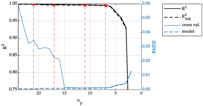
Figure 7 shows a representative example of the behavior of the two coefficients over the amount of remaining model parameters. This number also includes the additional constant parameter of the regression model.
Local maxima in are marked in red and can be seen as suitable models with high efficiency due to a good ratio of model quality and number of parameters. If no clear maximum can be found, a sudden drop off in both coefficients can also mark interesting models. Here, the remaining parameters contribute more to the quality of the model, than the ones just removed.
Both RMSE values in
Figure 7 result from a five-fold cross validation that the models of every optimization step are analyzed with. We use it to detect overfitting, where the model fails to perform with new data points that were not used in the original model fit. For cross validation, the available dataset is split into five subsets, whereof one is used as a validation set, while the four remaining sets are used as a training set. This process is repeated so that every subset is used as a validation set once. The resulting models are evaluated using the root mean square error (RMSE). Overfitting can be assumed if the average RMSE for the cross validation is of higher magnitude than the RMSE for the original model fit using the full dataset. This can be observed on the left-hand side of
Figure 7, where the models consist of more than 15 parameters.
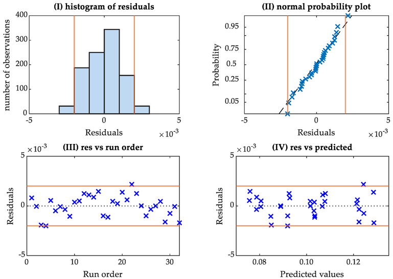
After finding a suitable model, its residuals are analyzed to validate three statistical prerequisites.
Figure 8 is a representative example depiction of the residual plots used for validation. Orange lines indicate measurement uncertainty of the test rig for CoF. Histogram (I) is supposed to resemble a bell curve. Residuals in the normal probability plot (II) should follow a diagonal. Additionally, if there are no apparent deviations to the right or left, these plots indicate normally distributed residuals. The residuals in the run order plot (III) should be evenly distributed around the x-axis, which implies the independence of the model errors. The last graph (IV) plots the residuals against the predicted values. An even distribution without any patterns indicates that the residuals have the same variance across all factor settings. Therefore, all necessary statistical prerequisites are fulfilled.
In addition to the ANOVA method for model reduction, we use stepwise regression. An automatic stepwise addition of factors is implemented in MatLab to build a regression model from any start model as simple as a single constant. We define criteria such as the p-value or the model efficiency . Corresponding thresholds for adding and removing factors are chosen to control the model optimization. In every step, the algorithm evaluates the available factors and adds the one with the highest positive impact on the chosen criterion. If no factor reaches the threshold for addition, the algorithm checks if any included factors became redundant due to the addition of others and now reach the threshold for removal. The resulting models are then also analyzed with a k-fold cross validation to avoid overfitting and residuals are also visually checked.
4. Results
4.1. Application of ANOVA with Cross Validation for Model Derivation
We apply the ANOVA method to the data of all tribological systems listed in
Table 4. It is possible to evaluate the influence of the investigated factors on the characteristic value
and to identify different models fulfilling the statistical requirements.
Before focusing on the other factors, the reproducibility of the data is verified for two tribological systems. For D88, MC-B the repeated measurements with the same clutch pack and for D117, MP-C the repetitions with two clutch pack are both split into two blocks. We then use this blocking in the ANOVA to evaluate the influence of the repetitions. In both cases, there is no significant difference between the first and the second run compared to the other factors with p-values above 0.05. The blocking can therefore be removed from the models.
We continue model identification with a full model containing all four main effects, the covariate and all interactions. The ANOVA method is used to find and remove the factors with the highest p-values. The order in which the factors are removed aligns with a preceding analysis using main effect and interaction diagrams. Due to a small main effect and weak interactions, the feeding oil flow rate is generally the first main factor to be removed. While the maximum differential speed has a similarly small main effect, its interactions are remarkable which is why they turned out to be more significant than the feeding oil flow rate.
The behavior of the two RMSE values strongly differ for a high number of parameters. RMSE in the fivefold cross validation is magnitudes higher than for the model fitted with the full original dataset. This can be interpreted as an indicator of overfitting and generally appears above 13 to 15 parameters (compare
Figure 7). Most of the suitable models according to the behavior of R
2 and
has a smaller number of parameters. Therefore, every ANOVA analysis leads to a range, where the number of parameters is low enough to avoid overfitting and high enough to allow for an accurate representation of the characteristic value µ
top. After validating the statistical prerequisites with the residual plots, the models in
Table 7 are chosen as the most promising ones. Friction systems D88, MC-B and D117, MP-C are used to derive models. Friction system D88, MP-A was only used for validation of those models and was not used for model derivation itself. Model 1 and model 2 show values of R
2 and
greater 99.5%, model 3 shows R
2 = 97.4% and
= 96.7%.
The analysis of D88, MC-B provides conclusive results, where the behavior of the coefficients and diagrams allows a clear decision on which models to choose. D88, MP-A shows a very strong dependency of CoF on steel plate temperature. However, maximum differential speed and its interactions are identified as insignificant early in the optimization process. The resulting model shows good behavior regarding residuals and has no dependency on the maximum differential speed. This correctly represents the friction behavior of this clutch, but it cannot be properly validated with the existing experimental design, which is strongly characterized by clutch speed ramps. D117, MP-C has a very consistent CoF. The analyzed factors show only little influence on the friction behavior. A suitable model with good residual behavior can be found at a sudden drop in both R2 and after the factor of feeding oil flow rate is removed. This drop suggests that the remaining factors contribute more to the quality of the model.
4.2. Application of Stepwise Regression with Cross Validation for Model Derivation
Using the dataset of D88, MC-B, we choose the p-value known from the ANOVA method as the first criterion for the stepwise regression algorithm. The threshold for adding a factor is set to p < 0.05 and the threshold for removal is p > 0.06. Starting from an empty model containing only a constant, the factors A, C and B are added consecutively. The order in which the factors are added makes the algorithm overlook the factor E that is known to be valuable from the ANOVA method before.
Consequently, factors A, C and E, which fulfill the criterion in the first step of the algorithm, are then used as part of the start model. With this configuration and the same thresholds, the algorithm manages to choose a final model equal to the first one in
Table 7. Using all five factors (A–E) as a starting model makes the algorithm choose the interactions DE, AC and CD, before removing the main effect B of feeding oil flow rate. This behavior matches the experience from the ANOVA method and the preceding analysis of main effect and interaction diagrams. The resulting model is equal to the second model in
Table 7. The fact that both models created with the manual ANOVA reappear in the automatic stepwise algorithm demonstrates the compatibility of the two methods. We then choose the change in the adjusted coefficient of determination
as an optimization criterion. This allows the model to be directly optimized for efficiency. The threshold for adding factors is set to
> 0, so that any improvement in model efficiency can be considered. After obtaining models with high
from the ANOVA method, the threshold for removal is set to −0.0001. Starting from an empty model with only one constant, the result is the same as before, where the algorithm overlooks the factor E. Using the factors A, C and E as a starting model results in the same order. Therefore, the algorithm chooses the first model in
Table 7 as before with the
p-value.
4.3. Model Validation
To validate the created models from
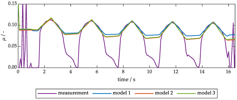
Table 7, we exemplarily compare the calculated CoF from these models with measurement data. CoF for load stage LS3 is determined with all models and compared to the measured data in
Figure 9. Between the five slip phases, all models calculate a high CoF even though the clutch speed is 0 rpm. One reason might be that the ANOVA and the model fit is executed with data within the range of 25 to 100 rpm. Therefore, the models cannot be applied to clutch speeds below 25 rpm.
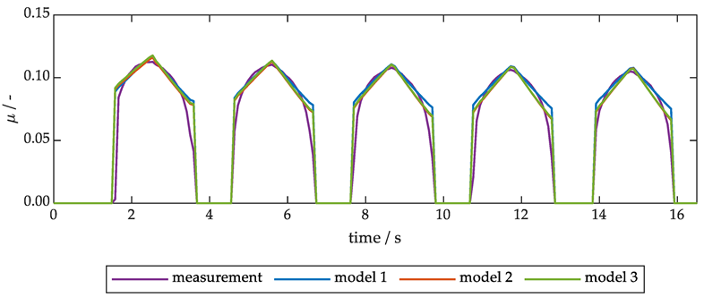
We restrict the visual model evaluation to clutch speeds above 1 rpm. For lower clutch speeds, CoF is set to 0.
Figure 10 shows that this adjustment only affects the area between the slip phases. At the beginning and at the end of each slip phase, the clutch speed is between 1 and 25 rpm. In this area of extrapolation, the models show the biggest deviations from the measurement and the biggest differences between each other. In the middle of the slip phase, the clutch speed is between 25 and 100 rpm. In this area, all models show a good representation of the measurement.
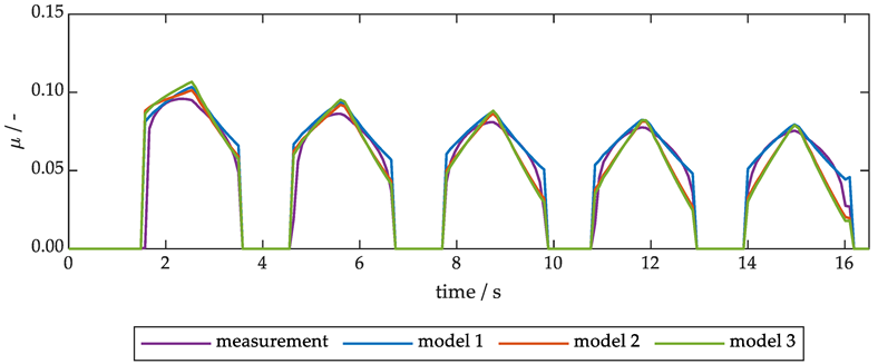
The load stage LS1 in
Figure 11 has higher pressure (3 N/mm²) compared to LS3, while the other factors stay the same. Higher pressure causes a faster rise in steel plate temperatures. Conversely, the CoF decreases over the slip phases. This behavior is well reproduced by all three models. In this high-pressure scenario, model 1 is closer to the measurement for the low-speed areas of the later slip phases. In the low-pressure scenario, models 2 and 3 performs better in these areas. Both plots show linear behavior of the models, which cannot perfectly match the non-linear behavior of the measured CoF.
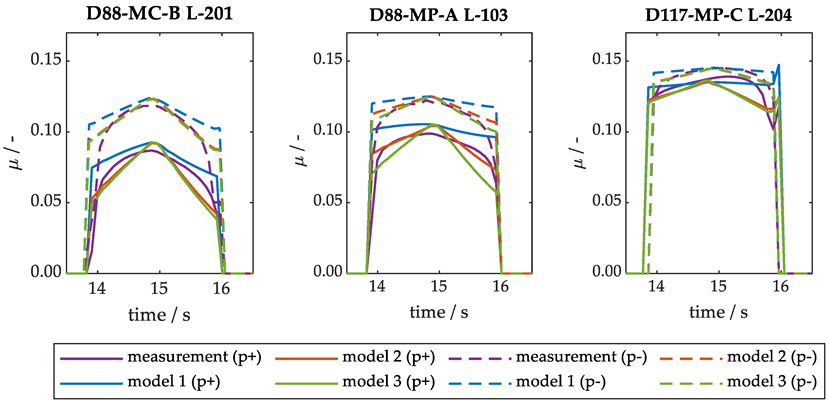
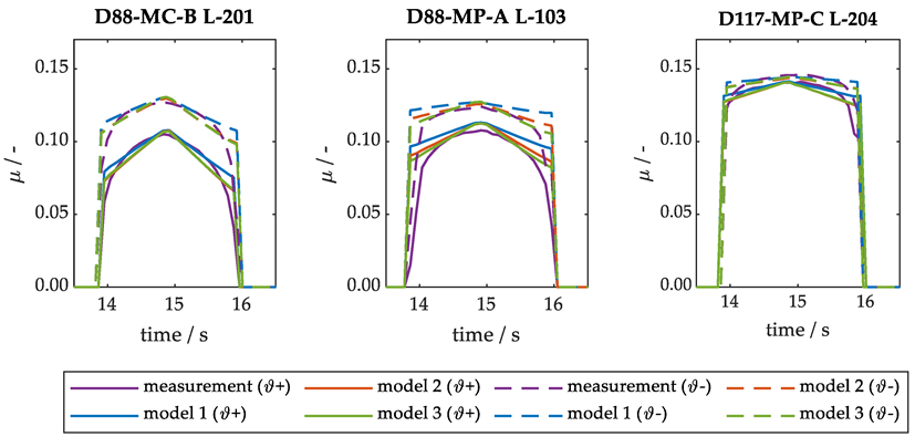
To compare transferability of the models between all tribological systems, only the last slip phases are observed.
Figure 12 shows the influence of clutch pressure on CoF with the dotted lines representing 1 N/mm² (p
−) and the solid lines representing 3 N/mm² (p
+). Although each model was derived for one specific friction system, all models react to the change in clutch pressure for all friction systems and can reproduce the level of CoF. Considering the behavior of CoF, the models perform differently in specific areas. In particular, the non-linear and asymmetric behavior of D117-MP-C L-204, caused by strong temperature dependence of CoF, is not reproduced by the linear models. Here, friction system D88-MP-A L-103 is used for validation only.
Figure 13 shows the influence of feeding oil temperature. Dotted lines represent feeding oil temperature 40 °C (ϑ
−) and solid lines 90 °C (ϑ
+). It can be observed that all models react to the change in oil temperature and can reproduce the level of the CoF.
5. Discussion
The presented approach uses experimental data to determine reasonable linear friction models. Both approaches, the ANOVA method and stepwise regression, show good compatibility and can be used to derive easy-to-use models. The derived models make it possible to analyze the analyzation of main influencing factors and consider their effects on CoF.
Here, a designed test plan helps to reduce the effort for experimental tests dramatically. Using ANOVA for the identification of suitable friction models also helps to determine the main effects on the friction behavior of the clutch system. To compare different clutch systems, the models can be derived for each clutch system individually. The formulation of the model itself supports the understanding of important effects but also the used coefficients. Further optimization could be possible by using physically motivated factors such as friction work and friction power instead of factors that can be directly controlled at the test rig such as differential speed and clutch pressure.
In addition, the presented modelling is suitable for operating modes with high energy input that show approximate linear friction behavior over sliding velocity. Strong non-linearities at very low sliding speeds or for curves of CoF over sliding velocity with significant maxima, for example, cannot be considered with the presented approach. Therefore, sophisticated, non-linear approaches should be considered. The linearity can also be checked in advance by performing tests at the center points of the tested load stages. Nevertheless, these nonlinearities are not relevant for thermal simulations of many clutches with paper or carbon-based friction lining. The energy input through friction work is very low at low sliding speeds and most clutch systems with the mentioned friction lining do not show significant maxima in their friction characteristic. Even for small non-linearities, the proposed methodology supports the identification of easy-to-use friction models with sufficient accuracy for thermal simulations, for example, with a significant reduction in experimental effort. A reasonable choice of the factor levels is crucial in finding the adequate model. Therefore, preliminary tests should be performed with the consideration of operational prerequisites.
The models respond properly to all changes in the factor levels in question. In addition, the resulting models show good correspondence to the measurements—even for more than one friction system. Therefore, the models are suitable as input models for thermal simulations with little effort for experimental investigations at the same time.
The procedure can easily be adapted, depending on the investigated conditions, and can also be used for other applications where experimental data are used for determining easy-to-use input models.
6. Conclusions
Since determining the friction behavior of wet disk clutches requires experimental investigation, a reasonable modeling approach for determining friction models is necessary. This paper presents an approach for identifying and validating linear friction models using ANOVA and stepwise regression. Three models are derived and discussed using three relevant clutch systems with paper- and carbon-based friction lining. Good compatibility of the ANOVA and stepwise regression approach is identified.
The proposed modeling allows for the derivation of easy-to-use linear friction models as inputs for thermal calculations, for example, with little experimental effort. Thus, linear models are found suitable for the investigated clutch systems in relevant operational modes. Experiments are characterized by the characteristic friction value µtop. Reasonable factors and corresponding factor levels are used for the experimental investigations.
By using DOE, the experimental effort could be reduced. ANOVA and stepwise regression both lead to the same linear friction models. Both approaches can support the interpretation of influencing factors. Due to the evaluation of reasonable performance criteria of the models, unnecessary factors for the modelling friction behavior can be identified and not considered in the model. When applying the presented modeling approach, the linearity of the underlying model should be checked in preliminary tests and in the model validation.
Author Contributions
Conceptualization, P.S., D.G. and E.S.; methodology, D.G., E.S. and L.P.-G.; software, E.S.; validation, P.S., D.G., E.S.; and L.P.-G.; formal analysis, P.S. and D.G.; investigation, D.G. and E.S.; resources, K.S.; data curation, D.G.; writing—original draft preparation, P.S., D.G. and E.S.; writing—review and editing, P.S., D.G., E.S., L.P.-G., K.V., H.P. and K.S.; visualization, P.S., D.G. and E.S.; supervision, D.G.; project administration, D.G.; funding acquisition, H.P., K.V. and K.S. All authors have read and agreed to the published version of the manuscript.
Funding
The proposed method was developed with data from experiments sponsored by the Research Association for Drive Technology e.V. (FVA). The presented experimental results are based on the research project FVA no. 413/V; self-financed by the FVA.
Data Availability Statement
The data presented in this study are available on request from the corresponding author.
Acknowledgments
The authors would like to thank Stephan Haug of TUM|Stat for advice on the statistical analysis. The authors would like to extend thanks for the sponsorship and support received from the FVA and the members of the project committee.
Conflicts of Interest
The authors declare no conflict of interest.
References
- Göppert, G. Adaptation of a wet clutch torque model in electrified drivelines. Forsch. Im Ing.-Eng. Res. 2021, 85, 913–922. [Google Scholar] [CrossRef]
- Hensel, M. Thermische Beanspruchbarkeit und Lebensdauerverhalten von nasslaufenden Lamellenkupplungen. Ph.D. Thesis, Technische Universität München, München, Germany, 2014. [Google Scholar]
- Lingesten, N.; Marklund, P.; Höglund, E. The influence of repeated high-energy engagements on the permeability of a paper-based wet clutch friction material. Proc. Inst. Mech. Eng. Part J. J. Eng. Tribol. 2017, 231, 1574–1582. [Google Scholar] [CrossRef]
- Voelkel, A.K.; Pflaum, H.; Stahl, K. Thermal Behavior and Cooling Conditions of Wet Multi-Plate Clutches in Modern Applications. In Proceedings of the STLE 72nd Annual Meeting and Exhibition of the Society of Tribologists and Lubrication Engineers, Atlanta, GA, USA, 21–25 May 2017. [Google Scholar]
- Ingram, M.; Noles, J.; Watts, R.; Harris, S.; Spikes, H.A. Frictional Properties of Automatic Transmission Fluids: Part I—Measurement of Friction-Sliding Speed Behavior. Tribol. Trans. 2010, 145–153. [Google Scholar] [CrossRef]
- Katsukawa, M. Effects of the Physical Properties of Resins on Friction Performance. In Proceedings of the WCX SAE World Congress Experience, Detroit, MI, USA, 9–11 April 2019; SAE International: Warrendale, PA, USA, 2019. [Google Scholar]
- Mäki, R.; Nyman, P.; Olsson, R.; Ganemi, B. Measurement and Characterization of Anti-shudder Properties in Wet Clutch Applications; SAE Technical Paper Nr. 2005-01-0878; SAE International: Warrendale, PA, USA, 2019. [Google Scholar] [CrossRef]
- Acuner, R.; Pflaum, H.; Stahl, K. Friction Screening Test for Wet Multiple Disc Clutches with Paper Type Friction Material. In Society of Tribologists and Lubrication Engineers Annual Meeting and Exhibition 2014; Society of Tribologists and Lubrication Engineers (STLE): Park Ridge, IL, USA, 2014; pp. 392–394. [Google Scholar]
- Groetsch, D.; Voelkel, K.; Pflaum, H.; Stahl, K. Real-time temperature calculation and temperature prediction of wet multi-plate clutches. Forsch. Im Ing.-Eng. Res. 2021, 85, 923–932. [Google Scholar] [CrossRef]
- Ma, B.; Yu, L.; Chen, M.; Li, H.Y.; Zheng, L.J. Numerical and experimental studies on the thermal characteristics of the clutch hydraulic system with provision for oil flow. Ind. Lubr. Tribol. 2019, 71, 733–740. [Google Scholar] [CrossRef]
- Björling, M.; Habchi, W.; Bair, S.; Larsson, R.; Marklund, P. Towards the true prediction of EHL friction. Tribol. Int. 2013, 66, 19–26. [Google Scholar] [CrossRef] [Green Version]
- Ingram, M.; Noles, J.; Watts, R.; Harris, S.; Spikes, H.A. Frictional Properties of Automatic Transmission Fluids: Part II—Origins of Friction-Sliding Speed Behavior. Tribol. Trans. 2010, 154–167. [Google Scholar] [CrossRef] [Green Version]
- Yoshizumi, F.; Tani, H.; Sanda, S. Simulation of the Friction Coefficient of Paper-Based Wet Clutch With Wavy Separators. J. Tribol. 2019, 141, 11702. [Google Scholar] [CrossRef]
- Wang, Y.; Guo, C.; Li, Y.; Li, G. Modelling the influence of velocity on wet friction-element friction in clutches. Ind. Lubr. Tribol. 2018, 70, 42–50. [Google Scholar] [CrossRef]
- Yang, Y.; Lam, R.C.; Fujii, T. Prediction of Torque Response During the Engagement of Wet Friction Clutch. In SAE Technical Paper Series, Proceedings of the SAE International Congress & Exposition, Detroit, MI, USA, 23–26 February 1998; SAE International: Warrendale, PA, USA, 1998. [Google Scholar]
- Gao, H.; Barber, G.C.; Shillor, M. Numerical Simulation of Engagement of a Wet Clutch With Skewed Surface Roughness. J. Tribol. 2002, 124, 305–312. [Google Scholar] [CrossRef]
- Davis, C.L.; Sadeghi, F.; Krousgrill, C.M. A simplified approach to modeling thermal effects in wet clutch engagement: Analytical and experimental comparison. J. Tribol. 2000, 122, 110–118. [Google Scholar] [CrossRef]
- Marklund, P.; Mäki, R.; Larsson, R.; Höglund, E.; Khonsari, M.M.; Jang, J. Thermal influence on torque transfer of wet clutches in limited slip differential applications. Tribol. Int. 2007, 40, 876–884. [Google Scholar] [CrossRef]
- Häggström, D.; Nyman, P.; Sellgren, U.; Björklund, S. Predicting friction in synchronizer systems. Tribol. Int. 2016, 97, 89–96. [Google Scholar] [CrossRef]
- Zhang, J.-L.; Ma, B.; Zhang, Y.-F.; Li, H.-Y. Simulation and Experimental Studies on the Temperature Field of a Wet Shift Clutch during One Engagement. In Proceedings of the 2009 International Conference on Computational Intelligence and Software Engineering, CiSE 2009, Wuhan, China, 11–13 December 2009; IEEE: Piscataway, NJ, USA, 2009; pp. 1–5, ISBN 978-1-4244-4507-3. [Google Scholar]
- Zhao, E.-h.; Ma, B.; Li, H.-Y. The Tribological Characteristics of Cu-Based Friction Pairs in a Wet Multidisk Clutch Under Nonuniform Contact. J. Tribol. 2018, 140, 011401. [Google Scholar] [CrossRef]
- Barr, M.; Srinivasan, K. Estimation of Wet Clutch Friction Parameters in Automotive Transmissions; SAE Technical Paper Series; SAE International: Warrendale, PA, USA, 2015. [Google Scholar]
- Wu, B.; Qin, D.; Hu, J.; Liu, Y. Experimental Data Mining Research on Factors Influencing Friction Coefficient of Wet Clutch. J. Tribol. 2021, 143, 121802. [Google Scholar] [CrossRef]
- Shui, H.; Zhang, Y.; Yang, H.; Upadhyay, D.; Fujii, Y. Machine Learning Approach for Constructing Wet Clutch Torque Transfer Function. SAE Int. J. Adv. Curr. Prac. Mobil. 2021, 3, 2738–2744. [Google Scholar]
- Stockinger, U.; Pflaum, H.; Stahl, K. Zeiteffiziente Methodik zur Ermittlung des Reibungsverhaltens nasslaufender Lamellenkupplungen mit Carbon-Reibbelag. Forsch. Im Ing.-Eng. Res. 2018, 82, 1–7. [Google Scholar] [CrossRef]
- Stockinger, U.; Groetsch, D.; Reiner, F.; Voelkel, K.; Pflaum, H.; Stahl, K. Friction behavior of innovative carbon friction linings for wet multi-plate clutches. Forsch. Im Ing.-Eng. Res. 2021, 2, 471. [Google Scholar] [CrossRef]
- Siebertz, K.; van Bebber, D.; Hochkirchen, T. Statistische Versuchsplanung: Design of Experiments (DoE), 2nd ed.; Vieweg: Kranzberg, Germany, 2017; ISBN 978-3-662-55743-3. [Google Scholar]
- Sudarsanam, N.; Frey, D.D. Using ensemble techniques to advance adaptive one-factor-at-a-time experimentation. Qual. Reliab. Engng. Int. 2011, 27, 947–957. [Google Scholar] [CrossRef]
- Frisch, H.; Schulz, R.K.; Sittig, K.; Dörfler, D.; Möller, K. Untersuchung der Drehmomentgleichförmigkeit durch geometrische Zwangserregung bei nasslaufenden Doppelkupplungen. In VDI-Berichte Nr. 2309, VDI-Fachtagung Kupplungen und Kupplungssysteme in Antrieben 2017, 2. VDI-Fachkonferenz Schwingungsreduzierung in mobilen Systemen 2017; Verein Deutscher Ingenieure (VDI): Ettlingen, Germany, 2017; pp. 359–370. [Google Scholar]
- Bischofberger, A.; Ott, S.; Albers, A. Einfluss von Betriebsgrößen auf die Schwingungsreduzierungswirkung im nasslaufenden Kupplungssystem: Empirische Modellbildung–Kennfelder und Skalierbarkeit. Forsch. Im Ing.-Eng. Res. 2021, 85, 933–944. [Google Scholar] [CrossRef]
- Mansouri, M.; Khonsari, M.M.; Holgerson, M.H.; Aung, W. Application of analysis of variance to wet clutch engagement. Proc. Inst. Mech. Eng. Part J. J. Eng. Tribol. 2002, 216, 117–125. [Google Scholar] [CrossRef]
- Meingaßner, G.J.; Pflaum, H.; Stahl, K. Test-Rig Based Evaluation of Performance Data of Wet Disk Clutches. In Proceedings of the 14th International CTI Symposium 2015, Berlin, Germany, 30 November–1 December 2015; pp. 1–11. [Google Scholar]
- Groetsch, D.; Motzet, R.; Voelkel, K.; Pflaum, H.; Stahl, K. Analysis of Oil Distribution and Reduction of Axial Force due to Oil Supply in a Multi-Plate Clutch. J. Serb. Tribol. Soc. 2022, 44, 268–282. [Google Scholar] [CrossRef]
- Baumgartner, A. Reibungsverhalten nasslaufender Lamellenkupplungen—Messunsicherheiten und Auswertemethoden. Master’s Thesis, Technical University of Munich, Munich, Germany, 2020. [Google Scholar]
- Polifke, W.; Kopitz, J. Wärmeübertragung: Grundlagen, Analytische und Numerische Methoden, 2. Aktual. Aufl.; Pearson Studium: München, Germany, 2009; ISBN 978-3-8273-7349-6. [Google Scholar]
- Voelkel, K. Charakterisierung des Einlaufverhaltens Nasslaufender Lamellenkupplungen. Ph.D. Thesis, Technical University of Munich, Munich, Germany, 2020. [Google Scholar]
Figure 1.
ZF/FZG KLP-260 test rig—schematic sketch according to [
32].
Figure 1.
ZF/FZG KLP-260 test rig—schematic sketch according to [
32].
Figure 2.
Steel and friction plates.
Figure 2.
Steel and friction plates.
Figure 3.
Position of thermocouples.
Figure 3.
Position of thermocouples.
Figure 4.
Courses of axial force (Fa) and differential speed (Δn) in non-steady slip.
Figure 4.
Courses of axial force (Fa) and differential speed (Δn) in non-steady slip.
Figure 5.
Explanation of µtop for two types of friction characteristics with equivalent values of µtop.
Figure 5.
Explanation of µtop for two types of friction characteristics with equivalent values of µtop.
Figure 6.
Trend plot of full factorial design of system D117/MP-C—values per cycle of varied parameters (oil injection temperature, nominal feeding oil flow rate, clutch pressure, maximum differential speed) and the measured variable (µtop).
Figure 6.
Trend plot of full factorial design of system D117/MP-C—values per cycle of varied parameters (oil injection temperature, nominal feeding oil flow rate, clutch pressure, maximum differential speed) and the measured variable (µtop).
Figure 7.
Representative example of behavior of coefficients R2 and
and RMSE values for model and cross validation over number of parameters np, D88 MC-B, L-201.
Figure 7.
Representative example of behavior of coefficients R2 and
and RMSE values for model and cross validation over number of parameters np, D88 MC-B, L-201.
Figure 8.
Representative example of residual plots, D88 MC-B, L-201 (model 1).
Figure 8.
Representative example of residual plots, D88 MC-B, L-201 (model 1).
Figure 9.
Comparison of measurement and simulation of CoF for load stage LS3 for three models fitted to D88, MC-B.
Figure 9.
Comparison of measurement and simulation of CoF for load stage LS3 for three models fitted to D88, MC-B.
Figure 10.
Comparison of measurement and simulation of CoF for load stage LS3 for three models fitted to D88, MC-B, restricted to ∆n > 1 rpm.
Figure 10.
Comparison of measurement and simulation of CoF for load stage LS3 for three models fitted to D88, MC-B, restricted to ∆n > 1 rpm.
Figure 11.
Comparison of measurement and simulation of CoF for load stage LS1 for three models fitted to D88, MC-B, restricted to ∆n > 1 rpm.
Figure 11.
Comparison of measurement and simulation of CoF for load stage LS1 for three models fitted to D88, MC-B, restricted to ∆n > 1 rpm.
Figure 12.
Comparison of measurement and simulation of CoF for load stages LS13 and LS15 with different pressures 1 N/mm² and 3 N/mm², restricted to ∆n > 1 rpm.
Figure 12.
Comparison of measurement and simulation of CoF for load stages LS13 and LS15 with different pressures 1 N/mm² and 3 N/mm², restricted to ∆n > 1 rpm.
Figure 13.
Comparison of measurement and simulation of CoF for load stage LS1 for three models fitted to D88, MC-B, restricted to ∆n > 1 rpm.
Figure 13.
Comparison of measurement and simulation of CoF for load stage LS1 for three models fitted to D88, MC-B, restricted to ∆n > 1 rpm.
Table 1.
Technical data of ZF/FZG KLP-260 test rig according to [
33].
Table 1.
Technical data of ZF/FZG KLP-260 test rig according to [
33].
| variable small fly wheels | J1 = 0.12 … 0.75 kgm² |
| basic inertia | J2 = 1.0 kgm² |
| plate diameters | d = 75 … 260 mm |
| max. torque | Tf,max = 2000 Nm |
| differential speed | Δn = 0 … 7000 rpm |
| slip speed | Δn = 0 … 140 rpm (creep drive)
Δn = 0 … 7000 rpm (main drive) |
| torque in slip mode | Tf,slip,max = 2000 Nm (creep drive)
Tf,slip,max = 60 Nm (main drive) |
| max. axial force | Fa,max = 40 kN |
| feeding oil temperature | ϑoil = 30 … 150 °C |
| feeding oil flow rate | oil = 0 … 7 L/min |
| feeding oil pressure | poil = 0 … 6 bar |
Table 2.
Overview of measurement accuracy on the ZF/FZG KLP-260 test rig (confidence level 95 %) extended version according to [
33].
Table 2.
Overview of measurement accuracy on the ZF/FZG KLP-260 test rig (confidence level 95 %) extended version according to [
33].
| Measured Variable | Uncertainty |
|---|
| axial force | +/− 1.3% |
| torque | +/− 0.4% |
| CoF | +/− 1.3% |
| speed (main drive) | +/− 0.2% |
| speed (creep drive) | +/− 0.9% |
| thermocouple type K class 1 | +/− 1.8 K (DIN)/+/− 0.3 K
(Estimated from calibration) |
| feeding oil pressure | +/− 0.1 bar |
| axial force | +/− 1.3% |
Table 3.
Technical data of the test lubricants.
Table 3.
Technical data of the test lubricants.
| Lubricant | Kinematic Viscosity at 40 °C | Kinematic Viscosity at 100 °C |
|---|
| L-103 | 35 mm²/s | 7 mm²/s |
| L-201 | 47 mm²/s | 9 mm²/s |
| L-205 | 30 mm²/s | 6 mm²/s |
Table 4.
Friction systems.
Table 4.
Friction systems.
| System | Mean Diameter | Friction Lining | Lubricant |
|---|
| D117 | 117 mm | MP-C | L-205 |
| D88 | 88 mm | MP-A | L-103 |
| D88 | 88 mm | MC-B | L-201 |
Table 5.
Parameters of load stages during running-in.
Table 5.
Parameters of load stages during running-in.
| Name | p/N/mm² | ∆n/rpm | Number of Slip Phases |
|---|
| E1 | 0.75 | 25 | 5 |
| E2 | 3.0 | 25 | 5 |
| E3 | 1.5 | 25 | 5 |
| E4 | 1–5 | 50 | 5 |
| E5 | 0.75 | 50 | 5 |
| E6 | 3.0 | 50 | 5 |
| EC | 0 | 20 | 1 |
Table 6.
Load stages and settings in the full-factorial design.
Table 6.
Load stages and settings in the full-factorial design.
| Symbol | A | B | C | D |
|---|
| Factor | Oil Injection Temperature | Feeding Oil
Flow | Clutch
Pressure | Max. Differential Speed |
|---|
| Low Level (−) | 40 °C | 0.25 mm³/mm²s | 1 N/mm² | 25 rpm |
|---|
| High Level (+) | 90 °C | 2 mm³/mm²s | 3 N/mm² | 100 rpm |
|---|
| Name | Factor Level |
|---|
| LS1 | + | + | + | + |
| LS2 | + | + | + | − |
| LS3 | + | + | − | + |
| LS4 | + | + | − | − |
| LS5 | + | − | + | + |
| LS6 | + | − | + | − |
| LS7 | + | − | − | + |
| LS8 | + | − | − | − |
| LS9 | − | + | + | + |
| LS10 | − | + | + | − |
| LS11 | − | + | − | + |
| LS12 | − | + | − | − |
| LS13 | − | − | + | + |
| LS14 | − | − | + | − |
| LS15 | − | − | − | + |
| LS16 | − | − | − | − |
Table 7.
Models chosen from ANOVA analysis.
Table 7.
Models chosen from ANOVA analysis.
Friction
System | Number of Parameters | Model |
|---|
| D88, MC-B | 7 | c0 + cA·A+cc·C+cD·D+cE·E+cAC·AC+cAD·AD (model 1) |
| D88, MC-B | 8 | c0 + cA·A + cc·C + cD·D + cE·E + cAC·AC + cCD·CD + cDE·DE (model 2) |
| D117, MP-C | 7 | c0 + cA·A + cc·C + cD·D + cE·E + cAC·AC + cDE·DE (model 3) |
| Publisher’s Note: MDPI stays neutral with regard to jurisdictional claims in published maps and institutional affiliations. |
© 2022 by the authors. Licensee MDPI, Basel, Switzerland. This article is an open access article distributed under the terms and conditions of the Creative Commons Attribution (CC BY) license (https://creativecommons.org/licenses/by/4.0/).

 ,
, 


