
Role of Ensemble Deep Learning for Brain Tumor Classification in Multiple Magnetic Resonance Imaging Sequence Data
 , ,
, ,
Abstract
:1. Introduction
The Significant Findings of the Proposed Work Are as Follows
- To develop an efficient computer-aided diagnosis tool for brain tumor grading.
- Finding a suitable MRI sequence for the brain tumor classification.
- Proposed ensemble algorithm based on majority voting.
2. Materials and Methods
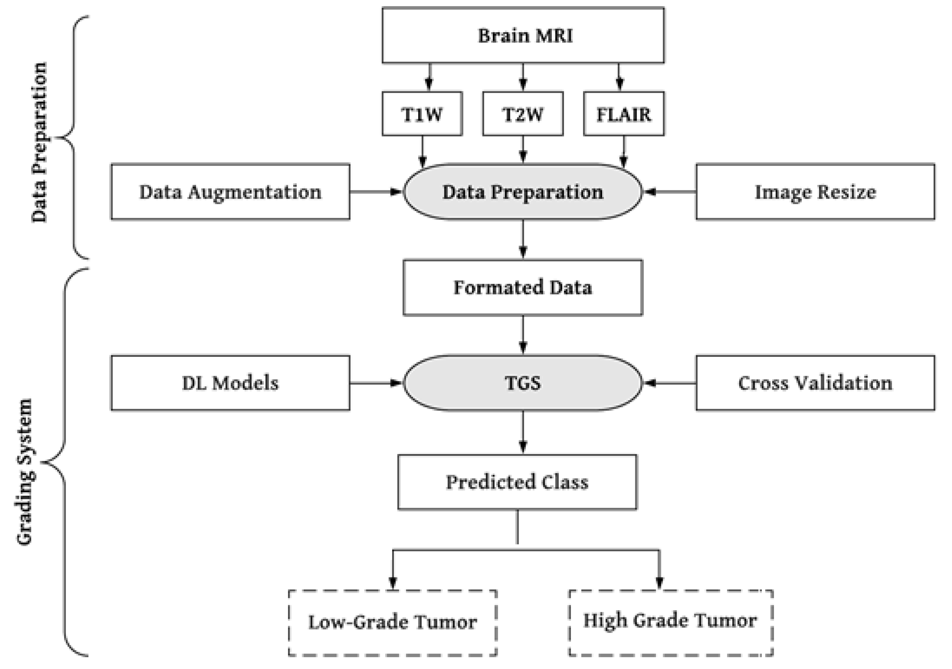
2.1. Data Preparation
2.2. Preprocessing
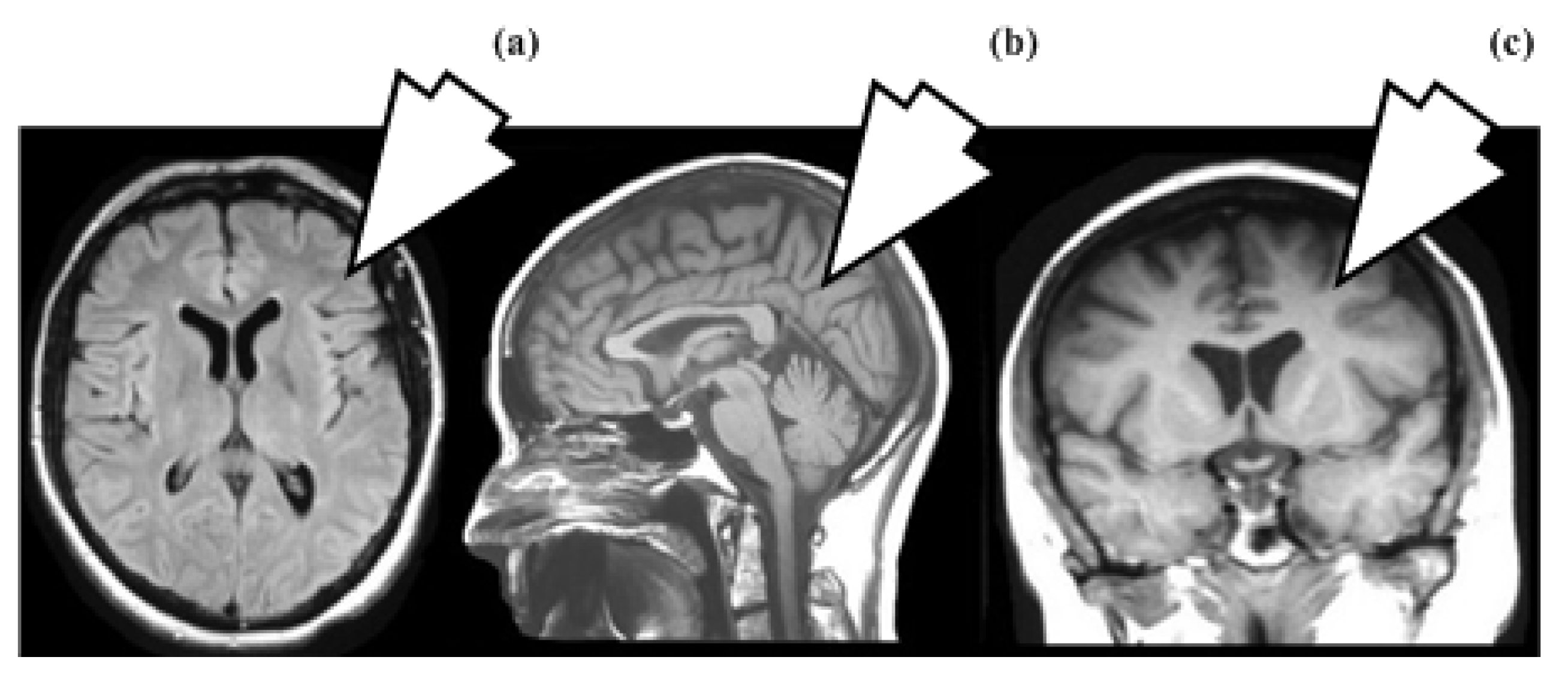
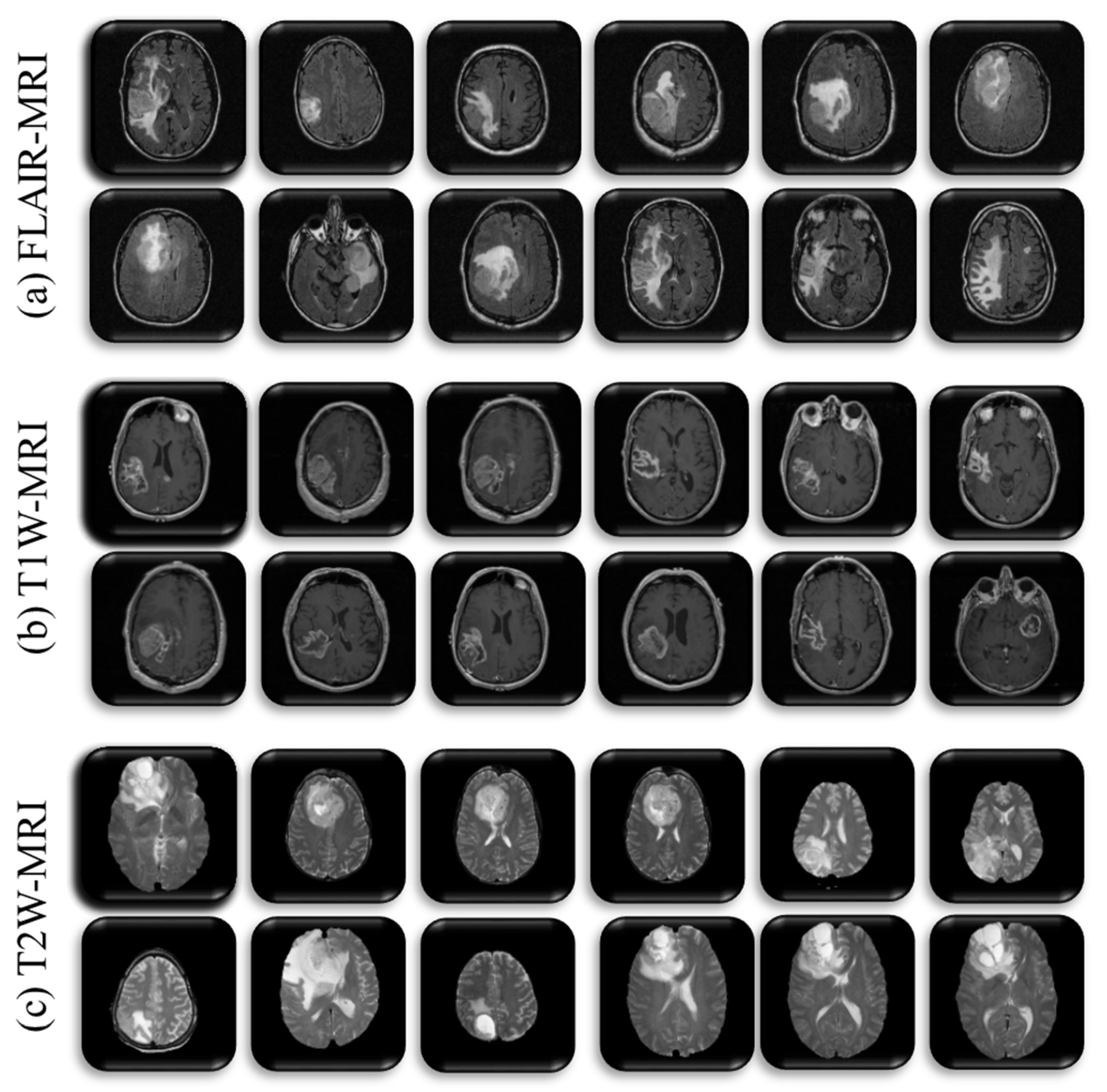
2.3. Clinical Relevance of MRI Sequence
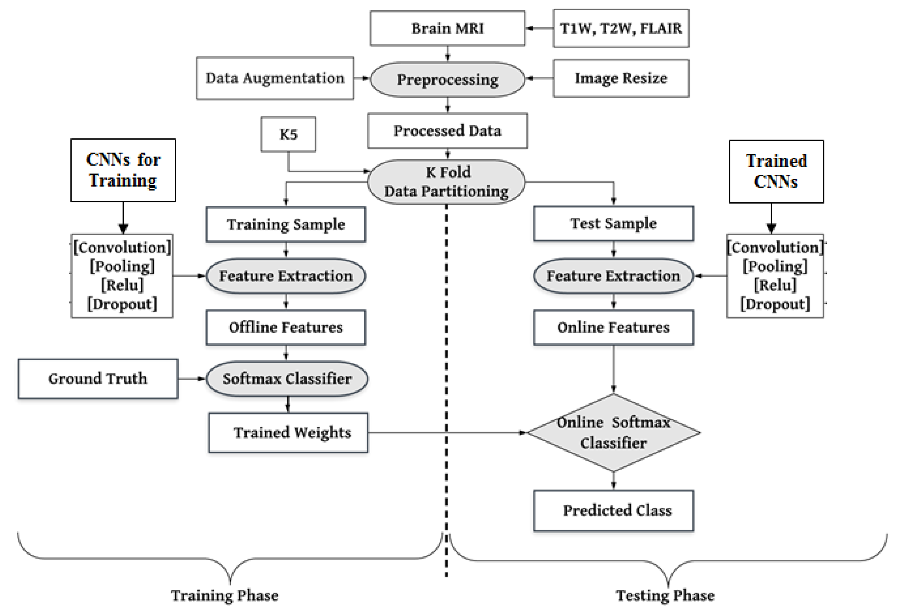
2.4. Methodology
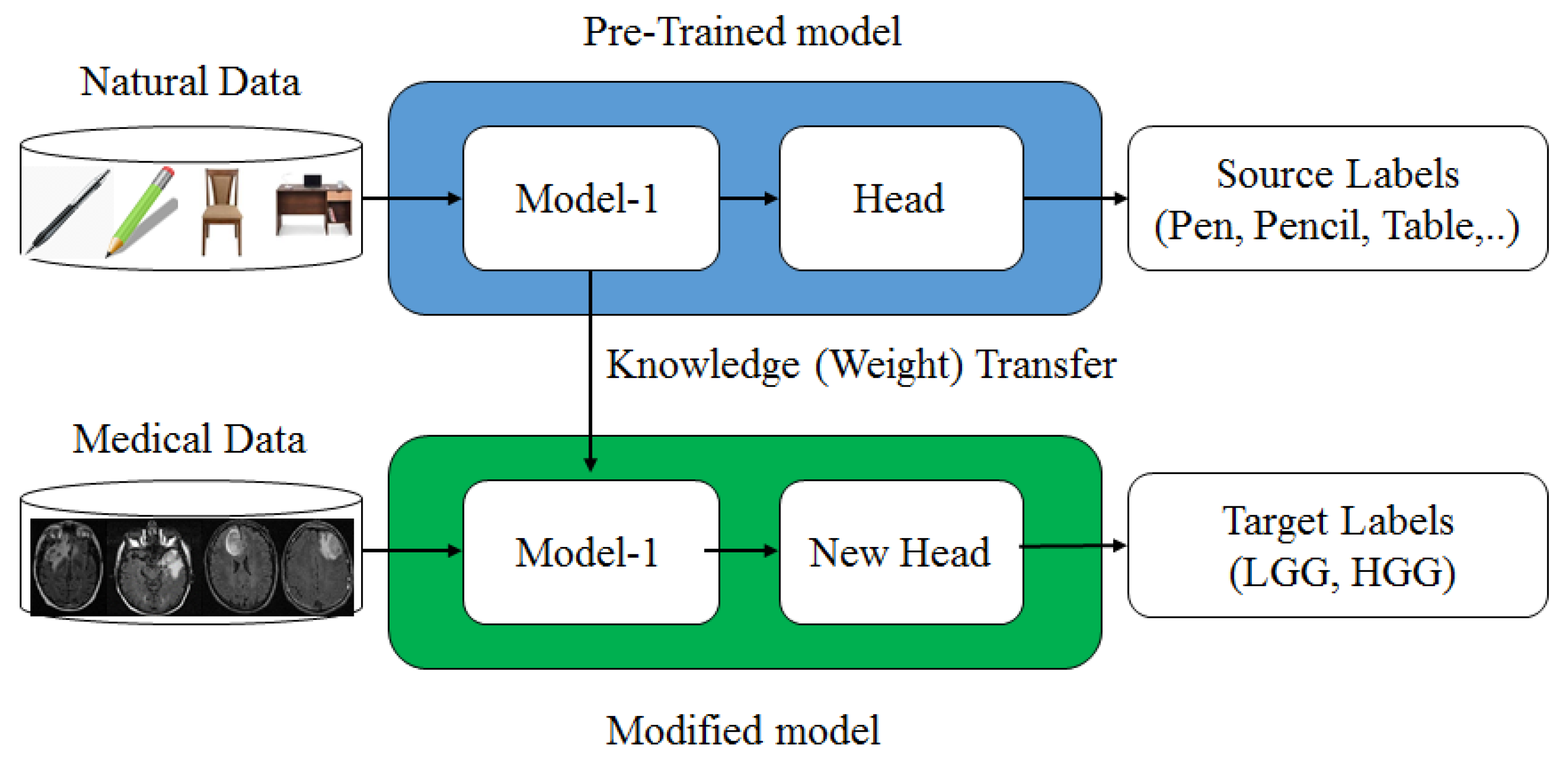
2.5. Transfer Learning
2.6. Pre-Trained Convolution Neural Network
2.6.1. AlexNet
2.6.2. VGGNet
2.6.3. GoogleNet
2.6.4. Residual Net
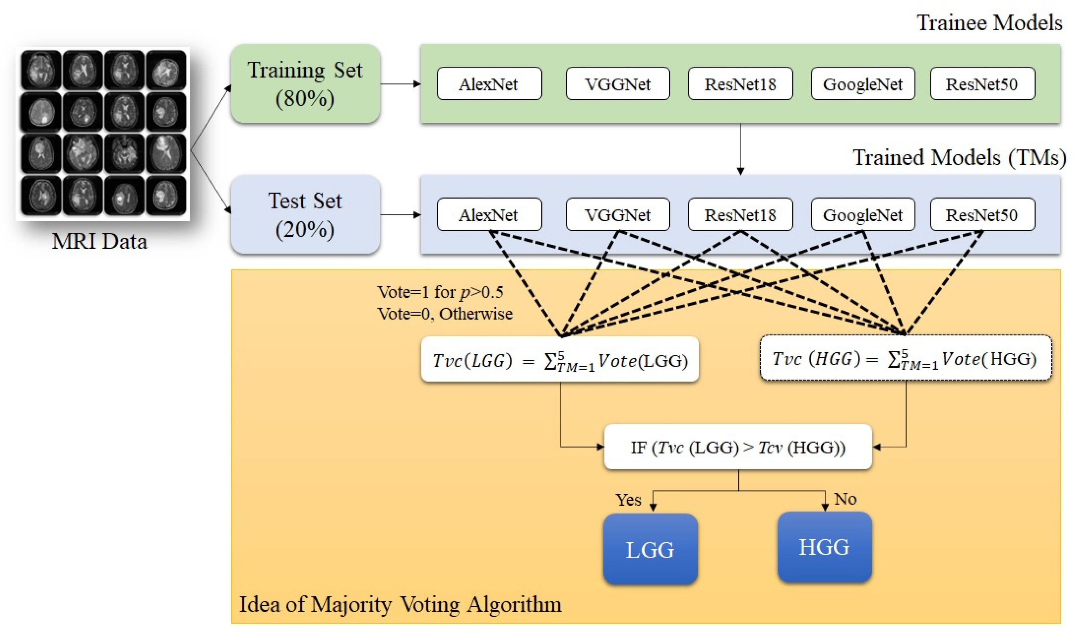
2.7. Majority Voting Algorithm (Algorithm 1)
| Algorithm 1: Majority Voting. |
| Input: n Models or classifiers, training samples with ground truth and test samples. |
| Output: Predicted class labels, label probability score, and performance evaluation. |
| Step 1. Train all n models on the same training set. |
| Step 2. Take a sample from test set and test it through trained model and predict the label in terms of probability score. |
| Step 3. Measure a model’s vote for each label by the following rule. IF Probability (label ‘LGG’) > 0.5 THEN Vote (LGG) = 1 and Vote (HGG) = 0. Otherwise, Vote (LGG) = 0 and Vote (HGG) = 1 |
| Step 5. Repeat step 2 and 3 for all the trained models. |
| Step 6. Calculate the total number of votes for each label predicted by all trained models by the following rule. IF (Total Vote ‘LGG’) > (Total Vote ‘HGG’) THEN Label ‘LGG’ will be predicted. Otherwise, Label ‘HGG’ will be predicted. |
| Step 7. Repeat Step 2 to Step 6 for all the test samples. |
| Step 8. Compare predicted labels of each sample to the actual ground truth and create confusion matrix. |
3. Results
3.1. Performance Evaluation of Dataset
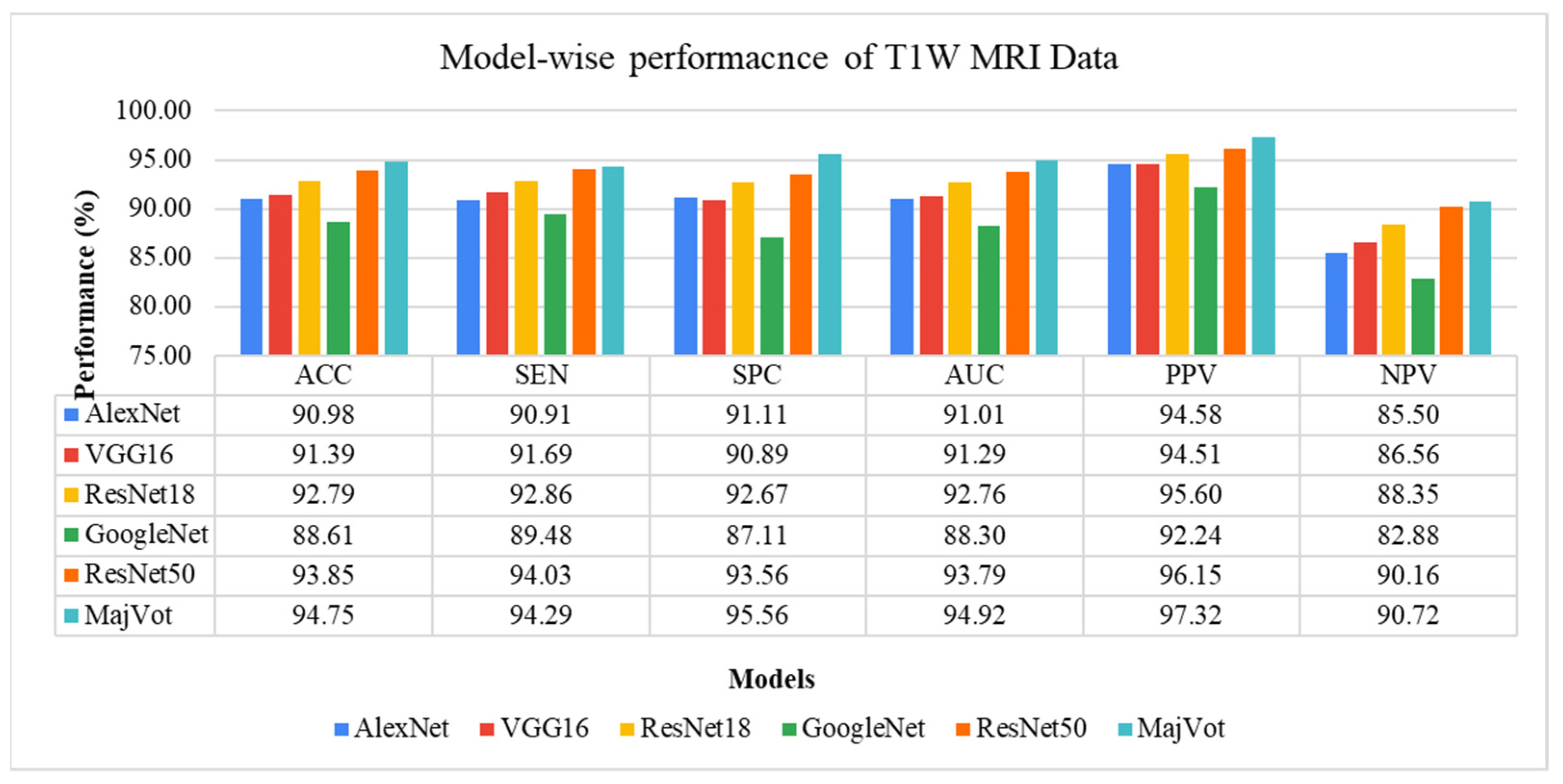
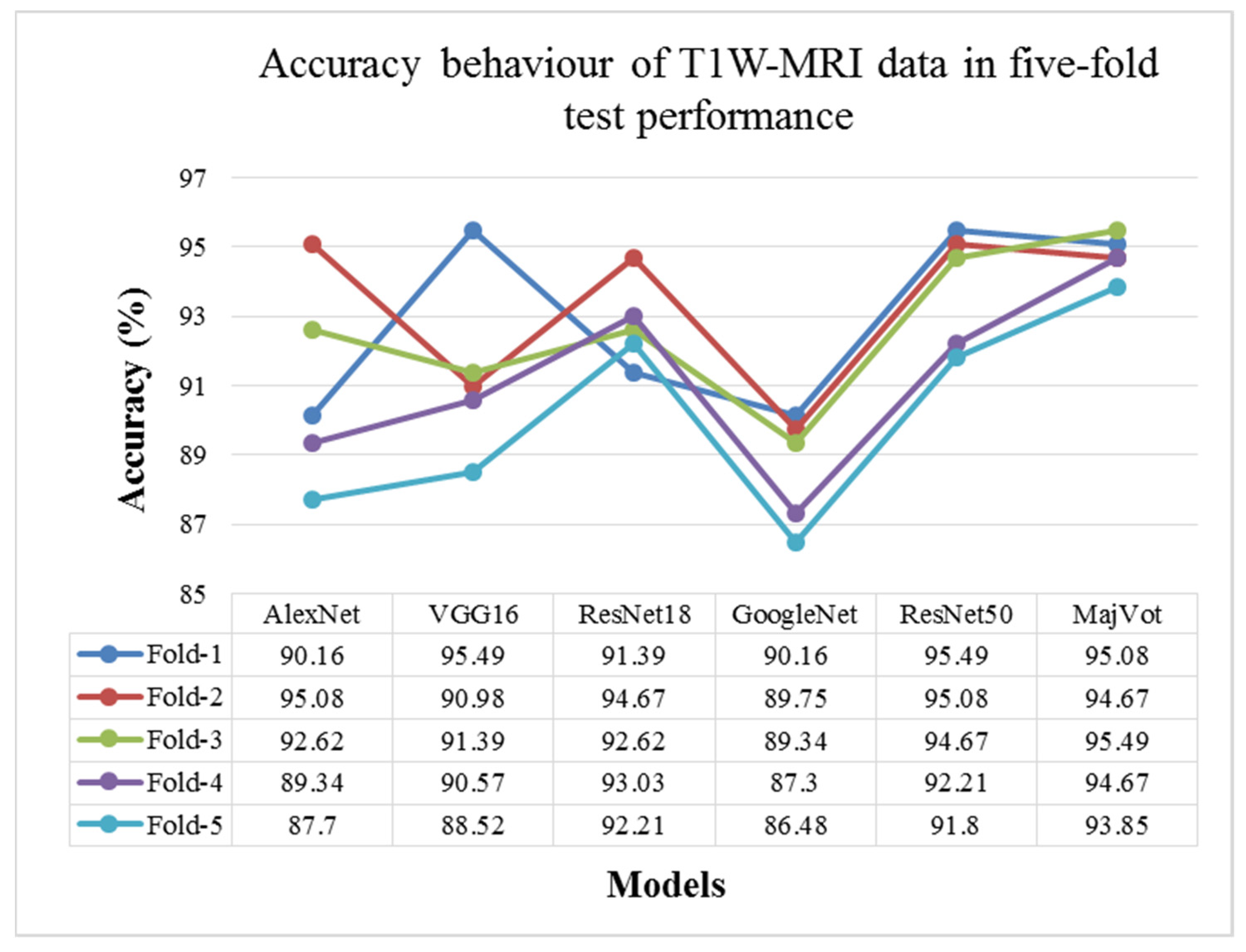
3.1.1. T1W-MRI Data Analysis
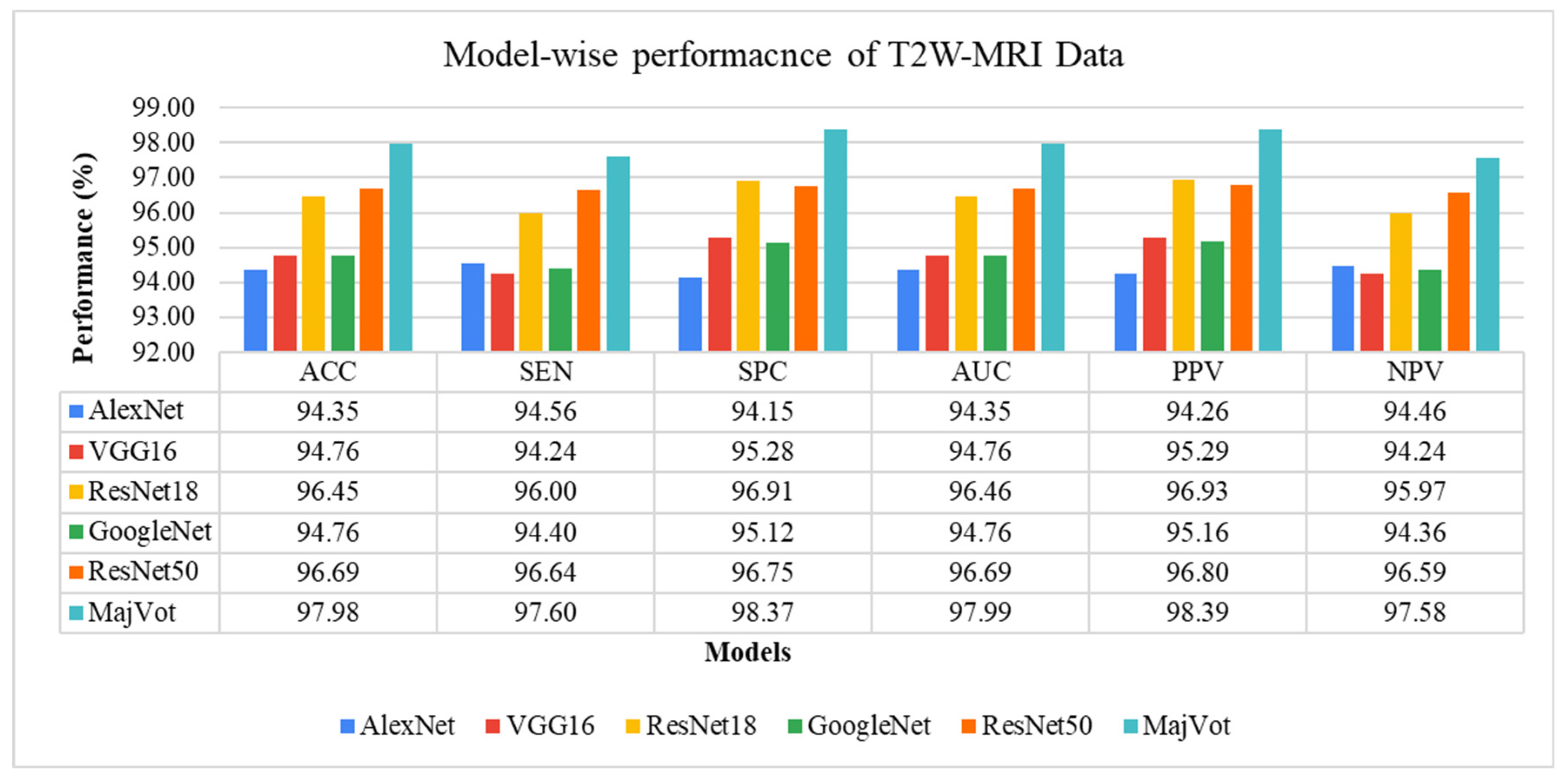
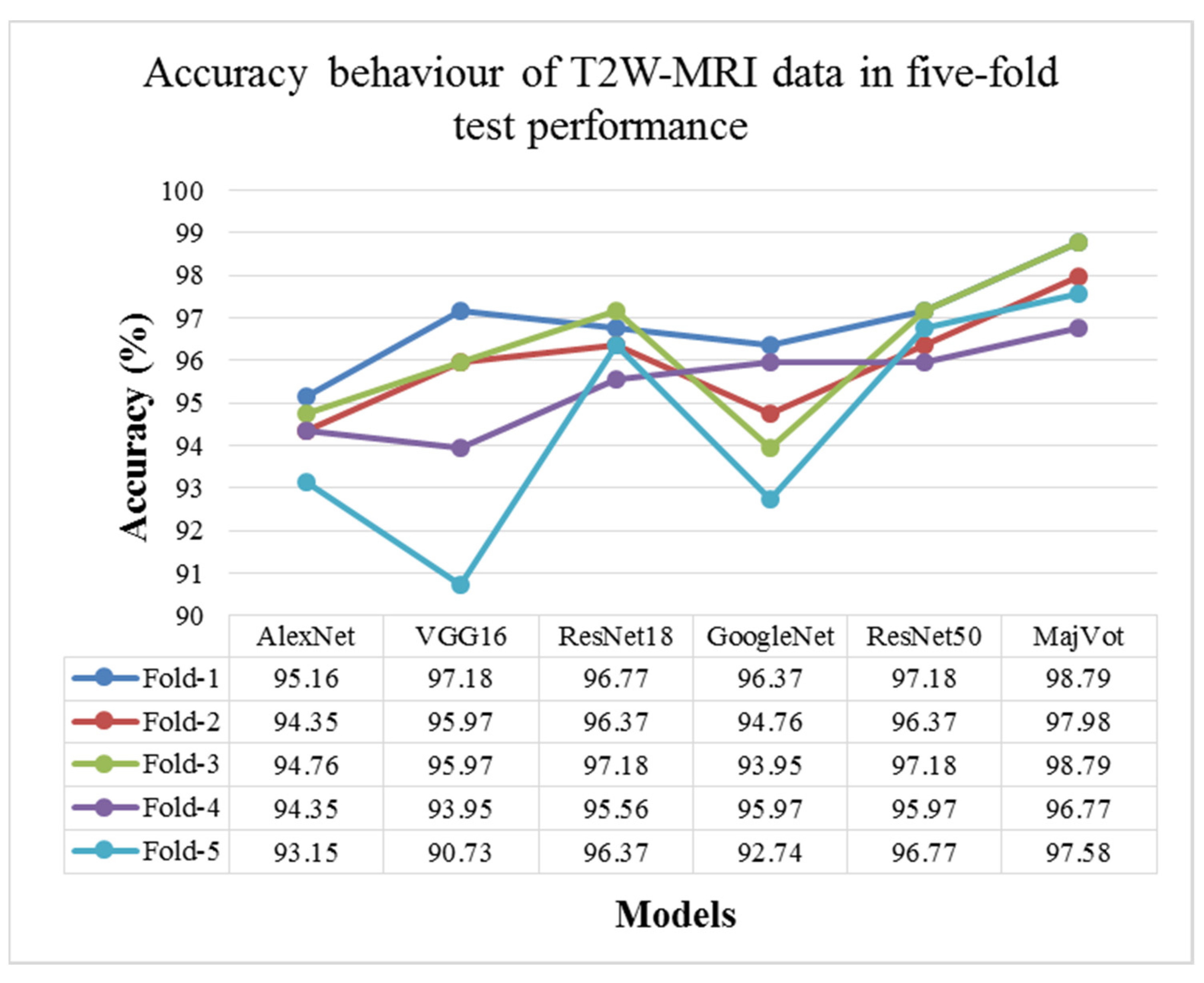
3.1.2. T2W-MRI Data Analysis
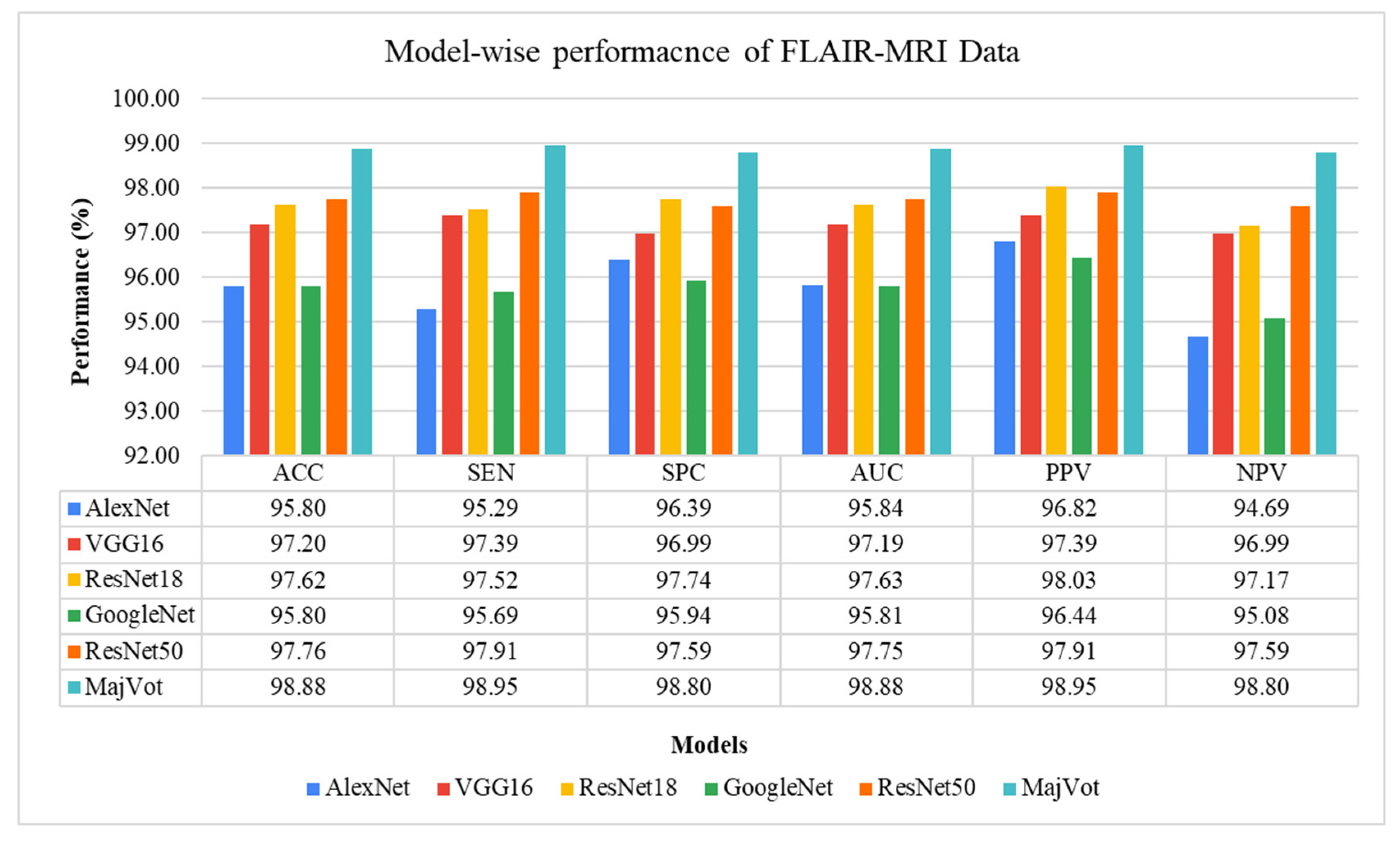
3.1.3. FLAIR-MRI Data Analysis
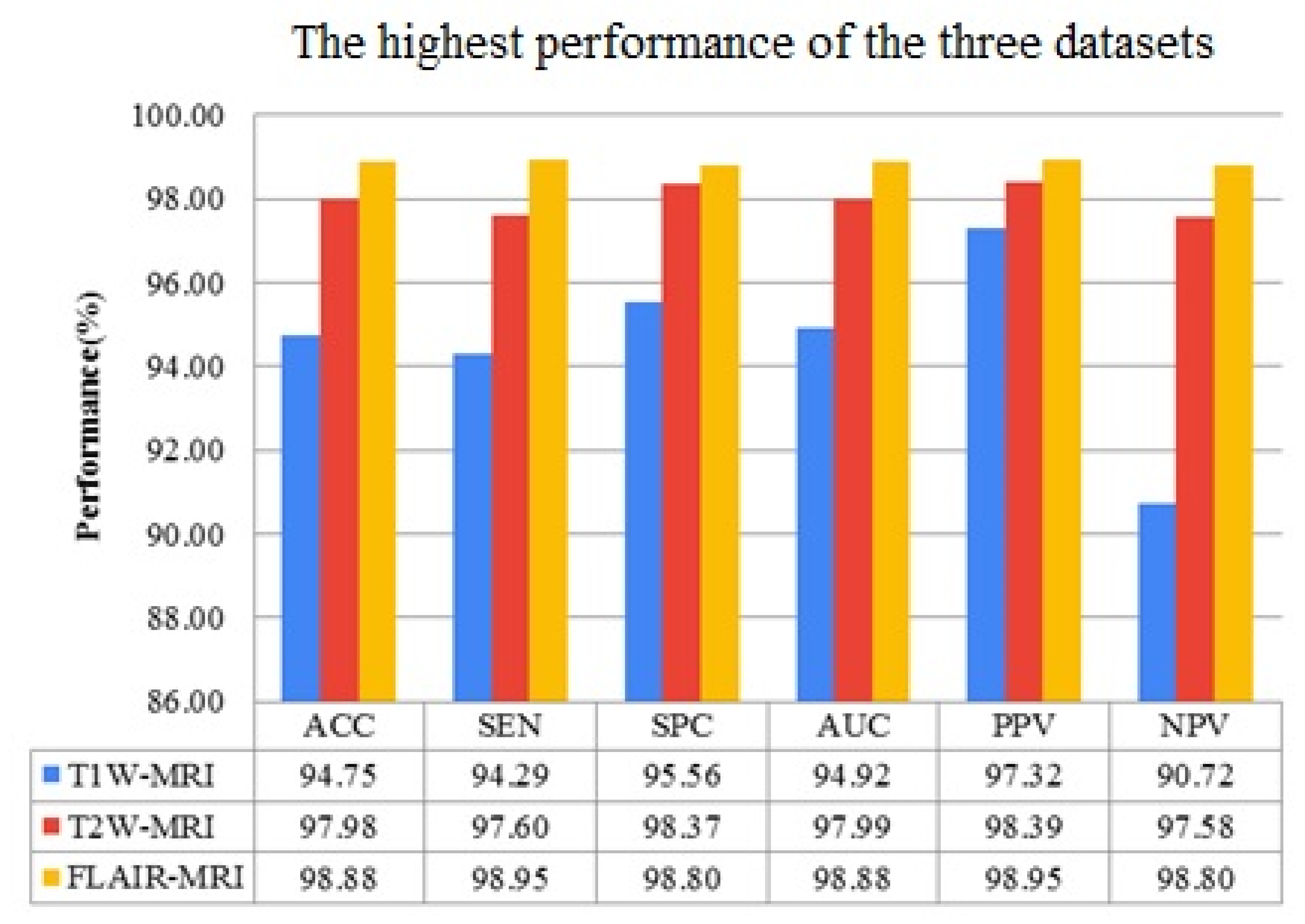
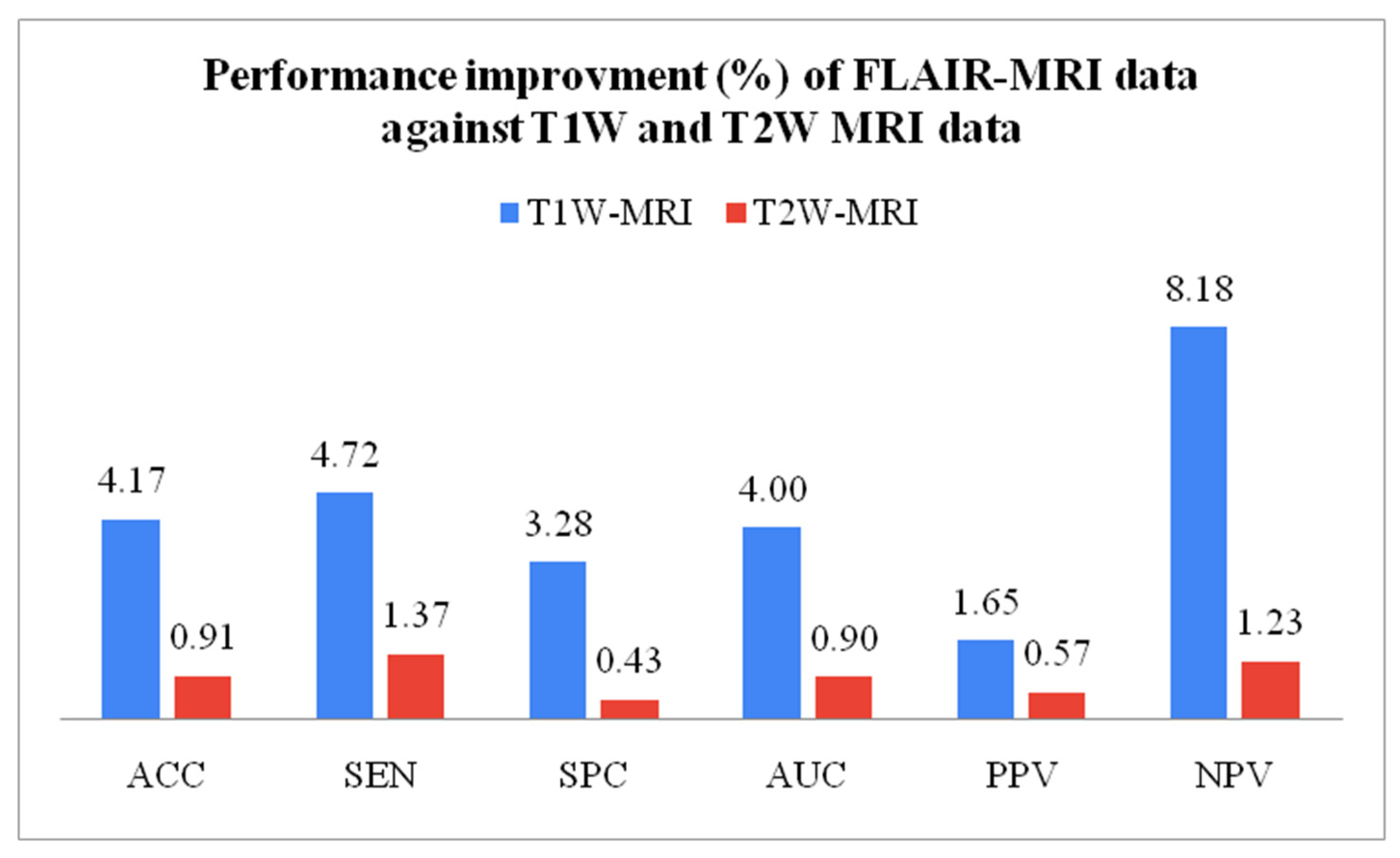
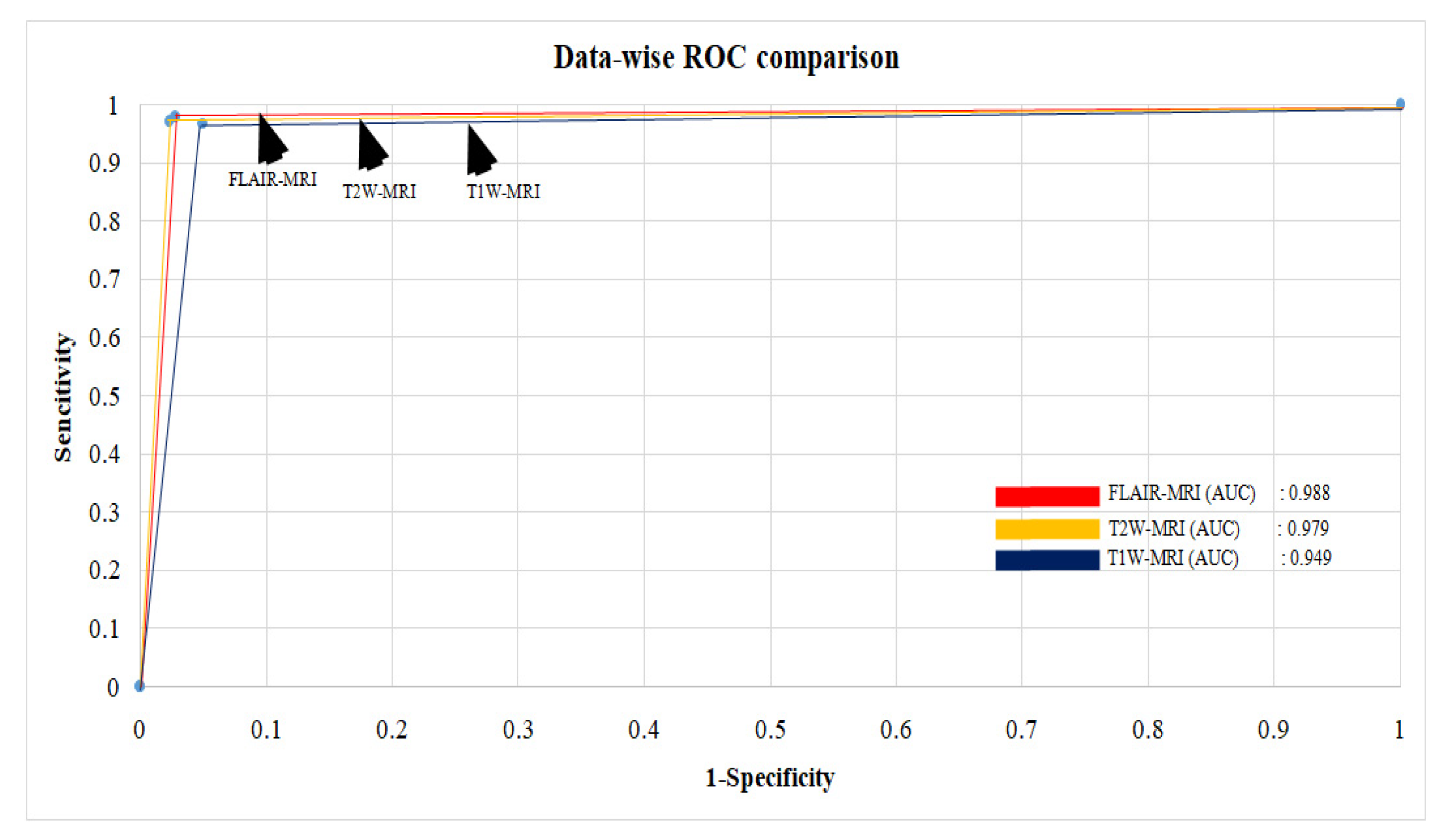
3.2. Performance Comparison of Three MRI Sequence Datasets
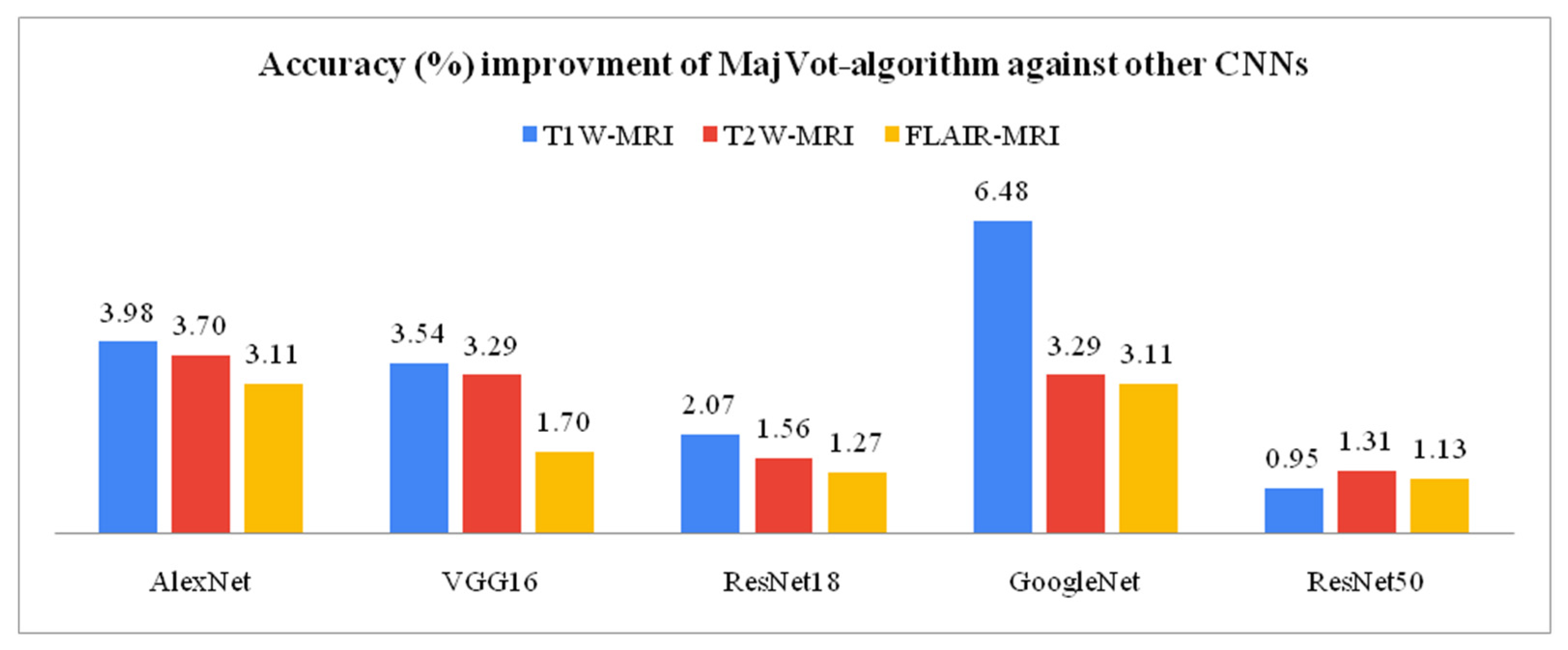
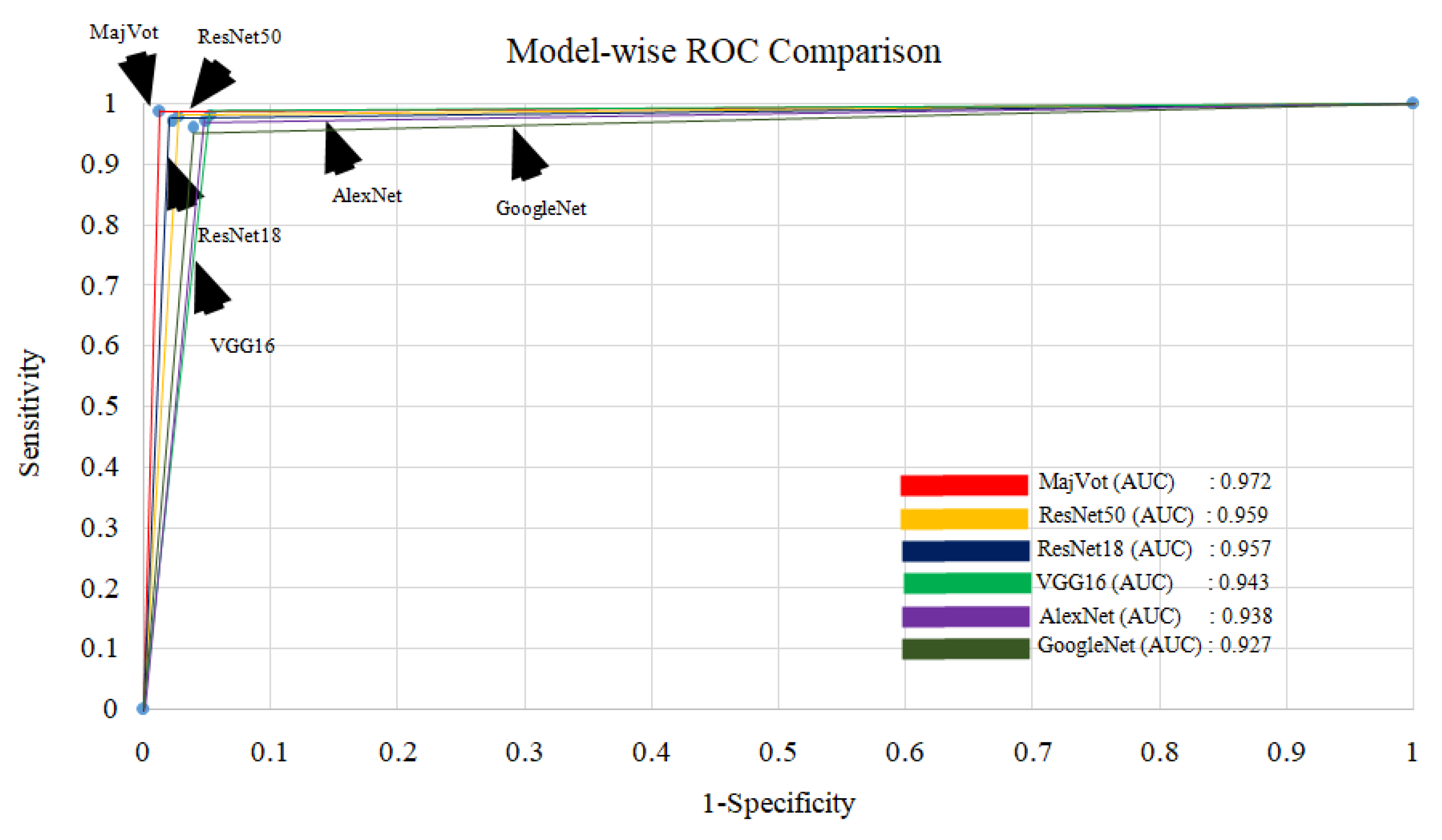
3.3. Model-Wise Performance Improvement
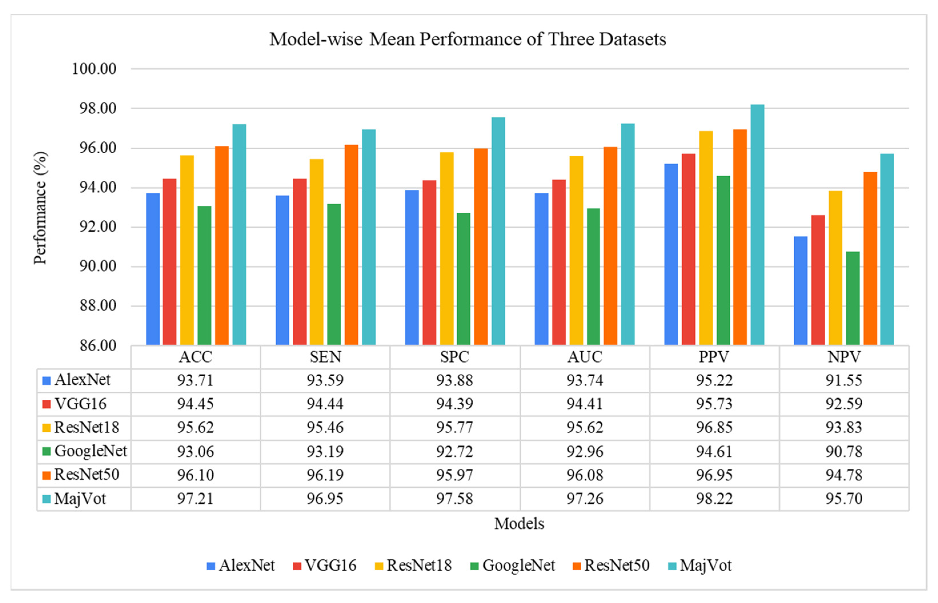
3.4. Experimental Protocol 4: Average Performance Analysis of Six Models and Three Datasets
4. Discussion
4.1. Special Note on Deep Learning Method
4.2. Clinical Applications of Magnetic Resonance Imaging
4.3. Strength, Weakness, and Future Extension
4.4. Benchmarking
5. Conclusions
Author Contributions
Funding
Institutional Review Board Statement
Informed Consent Statement
Data Availability Statement
Conflicts of Interest
Appendix A

| S.No. | Reference | Year | Summary | Novelty |
|---|---|---|---|---|
| 1 | Gupta et al. [78] | 2022 | A combined model with InceptionResNetV2 and Random Forest Tree was proposed for brain tumor classification. The model achieved 99% and 98% accuracy for the suggested tumor classification and detection models, respectively. | Two-model fusion |
| 2 | Haq E et al. [73] | 2022 | CNN and ML are combined to improve the accuracy of tumor segmentation and classification. The suggested technique attained the maximum classification accuracy of 98.3% between gliomas, meningiomas, and pituitary tumors. | Extracted features of CNN and ML models are fused |
| 3 | Srinivas et al. [74] | 2022 | Three CNN models are used in transfer learning mode for brain tumor classification: VGG16, ResNet50, and Inception-v3. The VGG16 has the best accuracy of 96% in classifying tumors as benign or malignant. | Compare three CNN models in transfer learning mode for brain tumor classification |
| 4 | Almalki et al. [75] | 2022 | Classified tumors using a linear machine learning classifiers (MLCs) model and a DL model. The proposed CNN with several layers (19, 22, and 25) is used to train the multiple MLCs in transfer learning to extract deep features. The accuracy of the CNN-SVM fused model was higher than that of previous MLC models. The fused model provided the highest accuracy (98%). | CNN-SVM mode fused for classification |
| 5 | Kibriya et al. [76] | 2022 | Suggested a new deep feature fusion-based multiclass brain tumor classification framework. Deep CNN features were extracted from transfer learning architectures such as AlexNet, GoogleNet, and ResNet18, and fused to create a single feature vector. SVM and KNN models are used as a classifier on this feature vector. The fused feature vector outperforms the individual vectors and system, achieving 99.7% highest accuracy. | Features of three CNNs are combined in a single feature vector |
| 6 | Gurunathan et al. [77] | 2022 | Suggested a CNN Deep net classifier for detecting brain tumors and classifying them into low and high grades. The suggested technique claims segmentation and classification accuracy of 99.4% and 99.5%, respectively. | Proposed a CNN Deep net classifier |
| Data | MRI (FLAIR) | MRI (T1W) | MRI (T2W) | |||
|---|---|---|---|---|---|---|
| #Fold | Training | Test | Training | Test | Training | Test |
| Fold 1 | 1143 | 287 | 717 | 180 | 991 | 249 |
| Fold 2 | 1143 | 287 | 717 | 180 | 991 | 249 |
| Fold 3 | 1143 | 287 | 717 | 180 | 991 | 249 |
| Fold 4 | 1143 | 287 | 717 | 180 | 991 | 249 |
| Fold 5 | 1143 | 287 | 717 | 180 | 991 | 249 |


Appendix B
| Experiment | Round# | ACC | SEN | SPC | AUC | PPV | NPV | ITR | TT (Minutes) |
|---|---|---|---|---|---|---|---|---|---|
| (AlexNet, T1W) | 1 | 90.16 | 90.91 | 88.89 | 89.90 | 93.33 | 85.11 | 9900 | 46.00 |
| 2 | 95.08 | 94.81 | 95.56 | 95.18 | 97.33 | 91.49 | 9900 | 45.00 | |
| 3 | 92.62 | 92.86 | 92.22 | 92.54 | 95.33 | 88.30 | 9900 | 47.00 | |
| 4 | 89.34 | 88.31 | 91.11 | 89.71 | 94.44 | 82.00 | 9900 | 55.00 | |
| 5 | 87.70 | 87.66 | 87.78 | 87.72 | 92.47 | 80.61 | 9900 | 54.00 | |
| MEAN | 90.98 | 90.91 | 91.11 | 91.01 | 94.58 | 85.50 | 9900 | 49.40 | |
| SD | 2.90 | 3.01 | 3.04 | 2.89 | 1.88 | 4.47 | 0.00 | 4.72 |
| Experiment | Round# | ACC | SEN | SPC | AUC | PPV | NPV | ITR | TT (Minutes) |
|---|---|---|---|---|---|---|---|---|---|
| (ResNet18, T1W) | 1 | 95.49 | 96.10 | 94.44 | 95.27 | 96.73 | 93.41 | 9900 | 315.00 |
| 2 | 90.98 | 90.91 | 91.11 | 91.01 | 94.59 | 85.42 | 9900 | 313.00 | |
| 3 | 91.39 | 90.26 | 93.33 | 91.80 | 95.86 | 84.85 | 9900 | 341.00 | |
| 4 | 90.57 | 92.21 | 87.78 | 89.99 | 92.81 | 86.81 | 9900 | 394.00 | |
| 5 | 88.52 | 88.96 | 87.78 | 88.37 | 92.57 | 82.29 | 9900 | 354.00 | |
| MEAN | 91.39 | 91.69 | 90.89 | 91.29 | 94.51 | 86.56 | 9900 | 343.40 | |
| SD | 2.54 | 2.73 | 3.08 | 2.57 | 1.83 | 4.17 | 0.00 | 33.20 |
| Experiment | Round# | ACC | SEN | SPC | AUC | PPV | NPV | ITR | TT (Minutes) |
|---|---|---|---|---|---|---|---|---|---|
| (ResNet18, T1W) | 1 | 91.39 | 91.56 | 91.11 | 91.33 | 94.63 | 86.32 | 9900 | 146.00 |
| 2 | 94.67 | 94.16 | 95.56 | 94.86 | 97.32 | 90.53 | 9900 | 92.00 | |
| 3 | 92.62 | 92.21 | 93.33 | 92.77 | 95.95 | 87.50 | 9900 | 117.00 | |
| 4 | 93.03 | 92.86 | 93.33 | 93.10 | 95.97 | 88.42 | 9900 | 86.00 | |
| 5 | 92.21 | 93.51 | 90.00 | 91.75 | 94.12 | 89.01 | 9900 | 112.00 | |
| MEAN | 92.79 | 92.86 | 92.67 | 92.76 | 95.60 | 88.35 | 9900 | 110.60 | |
| SD | 1.22 | 1.03 | 2.17 | 1.37 | 1.26 | 1.58 | 0.00 | 23.70 |
| Experiment | Round# | ACC | SEN | SPC | AUC | PPV | NPV | ITR | TT (Minutes) |
|---|---|---|---|---|---|---|---|---|---|
| (GoogleNet, T1W) | 1 | 90.16 | 90.26 | 90.00 | 90.13 | 93.92 | 84.38 | 9900 | 54.00 |
| 2 | 89.75 | 90.91 | 87.78 | 89.34 | 92.72 | 84.95 | 9900 | 98.00 | |
| 3 | 89.34 | 90.26 | 87.78 | 89.02 | 92.67 | 84.04 | 9900 | 112.00 | |
| 4 | 87.30 | 87.66 | 86.67 | 87.16 | 91.84 | 80.41 | 9900 | 141.00 | |
| 5 | 86.48 | 88.31 | 83.33 | 85.82 | 90.07 | 80.65 | 9900 | 121.00 | |
| MEAN | 88.61 | 89.48 | 87.11 | 88.30 | 92.24 | 82.88 | 9900 | 105.20 | |
| SD | 1.62 | 1.41 | 2.43 | 1.76 | 1.42 | 2.18 | 0.00 | 32.60 |
| Experiment | Round# | ACC | SEN | SPC | AUC | PPV | NPV | ITR | TT (Minutes) |
|---|---|---|---|---|---|---|---|---|---|
| (ResNet50, T1W) | 1 | 95.49 | 95.45 | 95.56 | 95.51 | 97.35 | 92.47 | 9900 | 230.00 |
| 2 | 95.08 | 95.45 | 94.44 | 94.95 | 96.71 | 92.39 | 9900 | 245.00 | |
| 3 | 94.67 | 94.16 | 95.56 | 94.86 | 97.32 | 90.53 | 9900 | 246.00 | |
| 4 | 92.21 | 92.86 | 91.11 | 91.98 | 94.70 | 88.17 | 9900 | 346.00 | |
| 5 | 91.80 | 92.21 | 91.11 | 91.66 | 94.67 | 87.23 | 9900 | 256.00 | |
| MEAN | 93.85 | 94.03 | 93.56 | 93.79 | 96.15 | 90.16 | 9900.00 | 264.60 | |
| SD | 1.71 | 1.48 | 2.28 | 1.82 | 1.36 | 2.40 | 0.00 | 46.44 |
| Experiment | Round# | ACC | SEN | SPC | AUC | PPV | NPV |
|---|---|---|---|---|---|---|---|
| (MajVot, T1W) | 1 | 95.08 | 94.81 | 95.56 | 95.18 | 97.33 | 91.49 |
| 2 | 94.67 | 94.16 | 95.56 | 94.86 | 97.32 | 90.53 | |
| 3 | 95.49 | 94.81 | 96.67 | 95.74 | 97.99 | 91.58 | |
| 4 | 94.67 | 94.16 | 95.56 | 94.86 | 97.32 | 90.53 | |
| 5 | 93.85 | 93.51 | 94.44 | 93.98 | 96.64 | 89.47 | |
| MEAN | 94.75 | 94.29 | 95.56 | 94.92 | 97.32 | 90.72 | |
| SD | 0.61 | 0.54 | 0.79 | 0.64 | 0.47 | 0.86 |
Appendix C
| Experiment | Round# | ACC | SEN | SPC | AUC | PPV | NPV | ITR | TT (Minutes) |
|---|---|---|---|---|---|---|---|---|---|
| (AlexNet, T2W) | 1 | 95.16 | 95.20 | 95.12 | 95.16 | 95.20 | 95.12 | 9900 | 46.00 |
| 2 | 94.35 | 94.40 | 94.31 | 94.35 | 94.40 | 94.31 | 9900 | 45.00 | |
| 3 | 94.76 | 96.00 | 93.50 | 94.75 | 93.75 | 95.83 | 9900 | 47.00 | |
| 4 | 94.35 | 94.40 | 94.31 | 94.35 | 94.40 | 94.31 | 9900 | 55.00 | |
| 5 | 93.15 | 92.80 | 93.50 | 93.15 | 93.55 | 92.74 | 9900 | 54.00 | |
| MEAN | 94.35 | 94.56 | 94.15 | 94.35 | 94.26 | 94.46 | 9900.00 | 49.40 | |
| SD | 0.75 | 1.19 | 0.68 | 0.75 | 0.65 | 1.15 | 0.00 | 4.72 |
| Experiment | Round# | ACC | SEN | SPC | AUC | PPV | NPV | ITR | TT (Minutes) |
|---|---|---|---|---|---|---|---|---|---|
| (ResNet18, T2W) | 1 | 97.18 | 96.80 | 97.56 | 97.18 | 97.58 | 96.77 | 9900 | 315.00 |
| 2 | 95.97 | 96.00 | 95.93 | 95.97 | 96.00 | 95.93 | 9900 | 313.00 | |
| 3 | 95.97 | 96.00 | 95.93 | 95.97 | 96.00 | 95.93 | 9900 | 341.00 | |
| 4 | 93.95 | 92.80 | 95.12 | 93.96 | 95.08 | 92.86 | 9900 | 394.00 | |
| 5 | 90.73 | 89.60 | 91.87 | 90.73 | 91.80 | 89.68 | 9900 | 354.00 | |
| MEAN | 94.76 | 94.24 | 95.28 | 94.76 | 95.29 | 94.24 | 9900.00 | 343.40 | |
| SD | 2.53 | 3.01 | 2.10 | 2.53 | 2.15 | 2.95 | 0.00 | 33.20 |
| Round# | ACC | SEN | SPC | AUC | PPV | NPV | ITR | TT (Minutes) | |
|---|---|---|---|---|---|---|---|---|---|
| (ResNet18, T2W) | 1 | 96.77 | 96.00 | 97.56 | 96.78 | 97.56 | 96.00 | 9900 | 146.00 |
| 2 | 96.37 | 96.00 | 96.75 | 96.37 | 96.77 | 95.97 | 9900 | 92.00 | |
| 3 | 97.18 | 96.80 | 97.56 | 97.18 | 97.58 | 96.77 | 9900 | 117.00 | |
| 4 | 95.56 | 95.20 | 95.93 | 95.57 | 95.97 | 95.16 | 9900 | 86.00 | |
| 5 | 96.37 | 96.00 | 96.75 | 96.37 | 96.77 | 95.97 | 9900 | 112.00 | |
| MEAN | 96.45 | 96.00 | 96.91 | 96.46 | 96.93 | 95.97 | 9900.00 | 110.60 | |
| SD | 0.60 | 0.57 | 0.68 | 0.60 | 0.67 | 0.57 | 0.00 | 23.70 |
| Experiment | Round# | ACC | SEN | SPC | AUC | PPV | NPV | ITR | TT (Minutes) |
|---|---|---|---|---|---|---|---|---|---|
| (GoogleNet, T2W) | 1 | 96.37 | 96.00 | 96.75 | 96.37 | 96.77 | 95.97 | 9900 | 315.00 |
| 2 | 94.76 | 94.40 | 95.12 | 94.76 | 95.16 | 94.35 | 9900 | 313.00 | |
| 3 | 93.95 | 93.60 | 94.31 | 93.95 | 94.35 | 93.55 | 9900 | 341.00 | |
| 4 | 95.97 | 96.00 | 95.93 | 95.97 | 96.00 | 95.93 | 9900 | 394.00 | |
| 5 | 92.74 | 92.00 | 93.50 | 92.75 | 93.50 | 92.00 | 9900 | 354.00 | |
| MEAN | 94.76 | 94.40 | 95.12 | 94.76 | 95.16 | 94.36 | 9900.00 | 343.40 | |
| SD | 1.48 | 1.70 | 1.29 | 1.48 | 1.30 | 1.68 | 0.00 | 33.20 |
| Experiment | Round# | ACC | SEN | SPC | AUC | PPV | NPV | ITR | TT (Minutes) |
|---|---|---|---|---|---|---|---|---|---|
| (ResNet50, T2W) | 1 | 97.18 | 96.80 | 97.56 | 97.18 | 97.58 | 96.77 | 9900 | 315.00 |
| 2 | 96.37 | 96.00 | 96.75 | 96.37 | 96.77 | 95.97 | 9900 | 313.00 | |
| 3 | 97.18 | 97.60 | 96.75 | 97.17 | 96.83 | 97.54 | 9900 | 341.00 | |
| 4 | 95.97 | 96.00 | 95.93 | 95.97 | 96.00 | 95.93 | 9900 | 394.00 | |
| 5 | 96.77 | 96.80 | 96.75 | 96.77 | 96.80 | 96.75 | 9900 | 354.00 | |
| MEAN | 96.69 | 96.64 | 96.75 | 96.69 | 96.80 | 96.59 | 9900.00 | 343.40 | |
| SD | 0.53 | 0.67 | 0.57 | 0.53 | 0.56 | 0.67 | 0.00 | 33.20 |
| Experiment | Round# | ACC | SEN | SPC | AUC | PPV | NPV |
|---|---|---|---|---|---|---|---|
| (MajVot, T2W) | 1 | 98.79 | 98.40 | 99.19 | 98.79 | 99.19 | 98.39 |
| 2 | 97.98 | 97.60 | 98.37 | 97.99 | 98.39 | 97.58 | |
| 3 | 98.79 | 98.40 | 99.19 | 98.79 | 99.19 | 98.39 | |
| 4 | 96.77 | 96.00 | 97.56 | 96.78 | 97.56 | 96.00 | |
| 5 | 97.58 | 97.60 | 97.56 | 97.58 | 97.60 | 97.56 | |
| MEAN | 97.98 | 97.60 | 98.37 | 97.99 | 98.39 | 97.58 | |
| SD | 0.86 | 0.98 | 0.81 | 0.85 | 0.81 | 0.97 |
Appendix D
| Experiment | Round# | ACC | SEN | SPC | AUC | PPV | NPV | ITR | TT (Minutes) |
|---|---|---|---|---|---|---|---|---|---|
| (AlexNet, FLAIR) | 1 | 96.50 | 96.73 | 96.24 | 96.49 | 96.73 | 96.24 | 9900 | 46.00 |
| 2 | 96.15 | 94.77 | 97.74 | 96.26 | 97.97 | 94.20 | 9900 | 45.00 | |
| 3 | 96.15 | 95.42 | 96.99 | 96.21 | 97.33 | 94.85 | 9900 | 47.00 | |
| 4 | 93.71 | 93.46 | 93.98 | 93.72 | 94.70 | 92.59 | 9900 | 55.00 | |
| 5 | 96.50 | 96.08 | 96.99 | 96.54 | 97.35 | 95.56 | 9900 | 54.00 | |
| MEAN | 95.80 | 95.29 | 96.39 | 95.84 | 96.82 | 94.69 | 9900.00 | 49.40 | |
| SD | 1.19 | 1.26 | 1.45 | 1.19 | 1.26 | 1.40 | 0.00 | 4.72 |
| Experiment | Round# | ACC | SEN | SPC | AUC | PPV | NPV | ITR | TT (Minutes) |
|---|---|---|---|---|---|---|---|---|---|
| (ResNet18, FLAIR) | 1 | 97.90 | 98.04 | 97.74 | 97.89 | 98.04 | 97.74 | 9900 | 315.00 |
| 2 | 97.55 | 97.39 | 97.74 | 97.56 | 98.03 | 97.01 | 9900 | 313.00 | |
| 3 | 97.20 | 97.39 | 96.99 | 97.19 | 97.39 | 96.99 | 9900 | 341.00 | |
| 4 | 96.15 | 96.73 | 95.49 | 96.11 | 96.10 | 96.21 | 9900 | 394.00 | |
| 5 | 97.20 | 97.39 | 96.99 | 97.19 | 97.39 | 96.99 | 9900 | 354.00 | |
| MEAN | 97.20 | 97.39 | 96.99 | 97.19 | 97.39 | 96.99 | 9900.00 | 343.40 | |
| SD | 0.65 | 0.46 | 0.92 | 0.67 | 0.79 | 0.54 | 0.00 | 33.20 |
| Experiment | Round# | ACC | SEN | SPC | AUC | PPV | NPV | ITR | TT (Minutes) |
|---|---|---|---|---|---|---|---|---|---|
| (ResNet18, FLAIR) | 1 | 98.60 | 98.69 | 98.50 | 98.59 | 98.69 | 98.50 | 9900 | 146.00 |
| 2 | 97.90 | 98.04 | 97.74 | 97.89 | 98.04 | 97.74 | 9900 | 92.00 | |
| 3 | 97.20 | 97.39 | 96.99 | 97.19 | 97.39 | 96.99 | 9900 | 117.00 | |
| 4 | 97.20 | 96.73 | 97.74 | 97.24 | 98.01 | 96.30 | 9900 | 86.00 | |
| 5 | 97.20 | 96.73 | 97.74 | 97.24 | 98.01 | 96.30 | 9900 | 112.00 | |
| MEAN | 97.62 | 97.52 | 97.74 | 97.63 | 98.03 | 97.17 | 9900.00 | 110.60 | |
| SD | 0.63 | 0.85 | 0.53 | 0.61 | 0.46 | 0.95 | 0.00 | 23.70 |
| Experiment | Round# | ACC | SEN | SPC | AUC | PPV | NPV | ITR | TT (Minutes) |
|---|---|---|---|---|---|---|---|---|---|
| (GoogleNet, FLAIR) | 1 | 96.15 | 96.08 | 96.24 | 96.16 | 96.71 | 95.52 | 9900 | 146.00 |
| 2 | 95.45 | 95.42 | 95.49 | 95.46 | 96.05 | 94.78 | 9900 | 92.00 | |
| 3 | 97.20 | 96.73 | 97.74 | 97.24 | 98.01 | 96.30 | 9900 | 117.00 | |
| 4 | 94.76 | 94.77 | 94.74 | 94.75 | 95.39 | 94.03 | 9900 | 86.00 | |
| 5 | 95.45 | 95.42 | 95.49 | 95.46 | 96.05 | 94.78 | 9900 | 112.00 | |
| MEAN | 95.80 | 95.69 | 95.94 | 95.81 | 96.44 | 95.08 | 9900.00 | 110.60 | |
| SD | 0.93 | 0.75 | 1.14 | 0.94 | 0.99 | 0.86 | 0.00 | 23.70 |
| Experiment | Round# | ACC | SEN | SPC | AUC | PPV | NPV | ITR | TT (Minutes) |
|---|---|---|---|---|---|---|---|---|---|
| (ResNet50, FLAIR) | 1 | 98.60 | 98.69 | 98.50 | 98.59 | 98.69 | 98.50 | 9900 | 146.00 |
| 2 | 97.90 | 98.04 | 97.74 | 97.89 | 98.04 | 97.74 | 9900 | 92.00 | |
| 3 | 97.20 | 97.39 | 96.99 | 97.19 | 97.39 | 96.99 | 9900 | 117.00 | |
| 4 | 97.90 | 98.04 | 97.74 | 97.89 | 98.04 | 97.74 | 9900 | 86.00 | |
| 5 | 97.20 | 97.39 | 96.99 | 97.19 | 97.39 | 96.99 | 9900 | 112.00 | |
| MEAN | 97.76 | 97.91 | 97.59 | 97.75 | 97.91 | 97.59 | 9900.00 | 110.60 | |
| SD | 0.59 | 0.55 | 0.63 | 0.59 | 0.55 | 0.63 | 0.00 | 23.70 |
| Experiment | Round# | ACC | SEN | SPC | AUC | PPV | NPV |
|---|---|---|---|---|---|---|---|
| (MajVot, FLAIR) | 1 | 99.30 | 99.35 | 99.25 | 99.30 | 99.35 | 99.25 |
| 2 | 98.60 | 98.69 | 98.50 | 98.59 | 98.69 | 98.50 | |
| 3 | 99.30 | 99.35 | 99.25 | 99.30 | 99.35 | 99.25 | |
| 4 | 99.30 | 99.35 | 99.25 | 99.30 | 99.35 | 99.25 | |
| 5 | 97.90 | 98.04 | 97.74 | 97.89 | 98.04 | 97.74 | |
| MEAN | 98.88 | 98.95 | 98.80 | 98.88 | 98.95 | 98.80 | |
| SD | 0.63 | 0.58 | 0.67 | 0.63 | 0.58 | 0.67 |
References
- Cancer Statistics. 2022. Available online: https://www.cancer.net/cancer-types/brain-tumor/statistics (accessed on 17 November 2022).
- Tandel, G.S.; Biswas, M.; Kakde, O.G.; Tiwari, A.; Suri, H.S.; Turk, M.; Laird, J.R.; Asare, C.K.; Ankrah, A.A.; Khanna, N.N.; et al. A Review on a Deep Learning Perspective in Brain Cancer Classification. Cancers 2019, 11, 111. [Google Scholar] [CrossRef] [PubMed] [Green Version]
- Gritsch, S.; Batchelor, T.T.; Castro, L.N.G. Diagnostic, therapeutic, and prognostic implications of the 2021 World Health Organization classification of tumors of the central nervous system. Cancer 2022, 128, 47–58. [Google Scholar] [CrossRef]
- Pereira, S.; Pinto, A.; Alves, V.; Silva, C.A. Brain Tumor Segmentation Using Convolutional Neural Networks in MRI Images. IEEE Trans. Med. Imaging 2016, 35, 1240–1251. [Google Scholar] [CrossRef]
- Xie, Y.; Zaccagna, F.; Rundo, L.; Testa, C.; Agati, R.; Lodi, R.; Manners, D.N.; Tonon, C. Convolutional Neural Network Techniques for Brain Tumor Classification (from 2015 to 2022): Review, Challenges, and Future Perspectives. Diagnostics 2022, 12, 1850. [Google Scholar] [CrossRef] [PubMed]
- American Society of Clinical Oncology. Brain Tumor Diagnosis. 2021. Available online: https://www.cancer.net/cancer-types/brain-tumor/diagnosis (accessed on 5 November 2021).
- Bauer, S.; Wiest, R.; Nolte, L.-P.; Reyes, M. A survey of MRI-based medical image analysis for brain tumor studies. Phys. Med. Biol. 2013, 58, R97. [Google Scholar] [CrossRef] [PubMed] [Green Version]
- Işın, A.; Direkoğlu, C.; Şah, M. Review of MRI-based Brain Tumor Image Segmentation Using Deep Learning Methods. Procedia Comput. Sci. 2016, 102, 317–324. [Google Scholar] [CrossRef] [Green Version]
- Balafar, M.A.; Ramli, A.R.; Saripan, M.I.; Mashohor, S. Review of brain MRI image segmentation methods. Artif. Intell. Rev. 2010, 33, 261–274. [Google Scholar] [CrossRef]
- Leung, D.; Han, X.; Mikkelsen, T.; Nabors, L.B. Role of MRI in Primary Brain Tumor Evaluation. J. Natl. Compr. Cancer Netw. 2014, 12, 1561–1568. [Google Scholar] [CrossRef] [PubMed] [Green Version]
- Kumar, R.; Srivastava, R.; Srivastava, S.K. Detection and Classification of Cancer from Microscopic Biopsy Images Using Clinically Significant and Biologically Interpretable Features. J. Med. Eng. 2015, 2015, 457906. [Google Scholar] [CrossRef] [PubMed]
- Veta, M.M.; Van Diest, P.J.; Kornegoor, R.; Huisman, A.; Viergever, M.A.; Pluim, J.P.W. Automatic Nuclei Segmentation in H&E Stained Breast Cancer Histopathology Images. PLoS ONE 2013, 8, e70221. [Google Scholar] [CrossRef]
- Gurcan, M.N.; Boucheron, L.E.; Can, A.; Madabhushi, A.; Rajpoot, N.M.; Yener, B. Histopathological Image Analysis: A Review. IEEE Rev. Biomed. Eng. 2009, 2, 147–171. [Google Scholar] [CrossRef] [PubMed] [Green Version]
- Wang, M.; He, X.; Chang, Y.; Sun, G.; Thabane, L. A sensitivity and specificity comparison of fine needle aspiration cytology and core needle biopsy in evaluation of suspicious breast lesions: A systematic review and meta-analysis. Breast 2017, 31, 157–166. [Google Scholar] [CrossRef] [PubMed]
- Moiin, A.; Neill, B.C. A novel punch biopsy technique without scissors or forceps. J. Am. Acad. Dermatol. 2021, 85, e71–e72. [Google Scholar] [CrossRef]
- Shives, T.C. Biopsy of soft-tissue tumors. Clin. Orthop. Relat. Res. 1993, 289, 32–35. [Google Scholar] [CrossRef]
- Tytgat, G.N.J.; Ignacio, J.-G. Technicalities of Endoscopic Biopsy. Endoscopy 1995, 27, 683–688. [Google Scholar] [CrossRef]
- Poulet, G.; Massias, J.; Taly, V. Liquid Biopsy: General Concepts. Acta Cytol. 2019, 63, 449–455. [Google Scholar] [CrossRef] [PubMed]
- Miller-Ocuin, J.L.; Fowler, B.B.; Coldren, D.L.; Chiba, A.; Levine, E.A.; Howard-McNatt, M. Is Excisional Biopsy Needed for Pure FEA Diagnosed on a Core Biopsy? Am. Surg. 2020, 86, 1088–1090. [Google Scholar] [CrossRef]
- Suri, J.S.; Puvvula, A.; Biswas, M.; Majhail, M.; Saba, L.; Faa, G.; Singh, I.M.; Oberleitner, R.; Turk, M.; Chadha, P.S.; et al. COVID-19 pathways for brain and heart injury in comorbidity patients: A role of medical imaging and artificial intelligence-based COVID severity classification: A review. Comput. Biol. Med. 2020, 124, 103960. [Google Scholar] [CrossRef] [PubMed]
- El-Baz, A.; Gimel’farb, G.; Suri, J.S. Stochastic Modeling for Medical Image Analysis; CRC Press: Boca Raton, FL, USA, 2015. [Google Scholar]
- Saba, L.; Biswas, M.; Kuppili, V.; Godia, E.C.; Suri, H.S.; Edla, D.R.; Omerzu, T.; Laird, J.R.; Khanna, N.N.; Mavrogeni, S.; et al. The present and future of deep learning in radiology. Eur. J. Radiol. 2019, 114, 14–24. [Google Scholar] [CrossRef] [PubMed]
- Suri, J.S.; Biswas, M.; Kuppili, V.; Saba, L.; Edla, D.R.; Suri, H.S.; Cuadrado-Godia, E.; Laird, J.R.; Marinhoe, R.T.; Sanches, J.M.; et al. State-of-the-art review on deep learning in medical imaging. Front. Biosci. 2019, 24, 380–406. [Google Scholar] [CrossRef] [PubMed]
- Maniruzzaman; Rahman, J.; Hasan, A.M.; Suri, H.S.; Abedin, M.; El-Baz, A.; Suri, J.S. Accurate Diabetes Risk Stratification Using Machine Learning: Role of Missing Value and Outliers. J. Med. Syst. 2018, 42, 92. [Google Scholar] [CrossRef] [PubMed] [Green Version]
- Zhou, M.; Scott, J.; Chaudhury, B.; Hall, L.; Goldgof, D.; Yeom, K.W.; Iv, M.; Ou, Y.; Kalpathy-Cramer, J.; Napel, S.; et al. Radiomics in Brain Tumor: Image Assessment, Quantitative Feature Descriptors, and Machine-Learning Approaches. Am. J. Neuroradiol. 2018, 39, 208–216. [Google Scholar] [CrossRef] [PubMed] [Green Version]
- Erickson, B.J.; Korfiatis, P.; Akkus, Z.; Kline, T.L. Machine Learning for Medical Imaging. Radiographics 2017, 37, 505–515. [Google Scholar] [CrossRef] [Green Version]
- Wang, Q.; Shi, Y.; Shen, D. Machine Learning in Medical Imaging. IEEE J. Biomed. Health Inform. 2019, 23, 1361–1362. [Google Scholar] [CrossRef] [Green Version]
- Litjens, G.; Kooi, T.; Bejnordi, B.E.; Setio, A.A.A.; Ciompi, F.; Ghafoorian, M.; van der Laak, J.A.W.M.; van Ginneken, B.; Sánchez, C.I. A survey on deep learning in medical image analysis. Med. Image Anal. 2017, 42, 60–88. [Google Scholar] [CrossRef] [PubMed] [Green Version]
- Chang, P.; Grinband, J.; Weinberg, B.D.; Bardis, M.; Khy, M.; Cadena, G.; Su, M.-Y.; Cha, S.; Filippi, C.G.; Bota, D.; et al. Deep-Learning Convolutional Neural Networks Accurately Classify Genetic Mutations in Gliomas. Am. J. Neuroradiol. 2018, 39, 1201–1207. [Google Scholar] [CrossRef] [PubMed] [Green Version]
- Nalawade, S.; Murugesan, G.K.; Vejdani-Jahromi, M.; Fisicaro, R.A.; Yogananda, C.G.B.; Wagner, B.; Mickey, B.; Maher, E.; Pinho, M.C.; Fei, B.; et al. Classification of brain tumor isocitrate dehydrogenase status using MRI and deep learning. J. Med. Imaging 2019, 6, 046003. [Google Scholar] [CrossRef]
- Ghiasi, M.M.; Zendehboudi, S.; Mohsenipour, A.A. Decision tree-based diagnosis of coronary artery disease: CART model. Comput. Methods Programs Biomed. 2020, 192, 105400. [Google Scholar] [CrossRef] [PubMed]
- Araki, T.; Ikeda, N.; Shukla, D.; Jain, P.K.; Londhe, N.D.; Shrivastava, V.K.; Banchhor, S.K.; Saba, L.; Nicolaides, A.; Shafique, S.; et al. PCA-based polling strategy in machine learning framework for coronary artery disease risk assessment in intravascular ultrasound: A link between carotid and coronary grayscale plaque morphology. Comput. Methods Programs Biomed. 2016, 128, 137–158. [Google Scholar] [CrossRef] [PubMed]
- Dagliati, A.; Marini, S.; Sacchi, L.; Cogni, G.; Teliti, M.; Tibollo, V.; De Cata, P.; Chiovato, L.; Bellazzi, R. Machine Learning Methods to Predict Diabetes Complications. J. Diabetes Sci. Technol. 2018, 12, 295–302. [Google Scholar] [CrossRef]
- Wu, Y.-T.; Zhang, C.-J.; Mol, B.W.; Kawai, A.; Li, C.; Chen, L.; Wang, Y.; Sheng, J.-Z.; Fan, J.-X.; Shi, Y.; et al. Early Prediction of Gestational Diabetes Mellitus in the Chinese Population via Advanced Machine Learning. J. Clin. Endocrinol. Metab. 2021, 106, e1191–e1205. [Google Scholar] [CrossRef] [PubMed]
- Shrivastava, V.K.; Londhe, N.D.; Sonawane, R.S.; Suri, J.S. A novel and robust Bayesian approach for segmentation of psoriasis lesions and its risk stratification. Comput. Methods Programs Biomed. 2017, 150, 9–22. [Google Scholar] [CrossRef] [PubMed]
- Shrivastava, V.; Londhe, N.D.; Sonawane, R.; Suri, J.S. Reliable and accurate psoriasis disease classification in dermatology images using comprehensive feature space in machine learning paradigm. Expert Syst. Appl. 2015, 42, 6184–6195. [Google Scholar] [CrossRef]
- Acharya, U.R.; Faust, O.; Sree, S.V.; Molinari, F.; Garberoglio, R.; Suri, J.S. Cost-Effective and Non-Invasive Automated Benign & Malignant Thyroid Lesion Classification in 3D Contrast-Enhanced Ultrasound Using Combination of Wavelets and Textures: A Class of ThyroScan™ Algorithms. Technol. Cancer Res. Treat. 2011, 10, 371–380. [Google Scholar] [CrossRef] [PubMed] [Green Version]
- Acharya, U.R.; Sree, S.V.; Krishnan, M.M.R.; Molinari, F.; Garberoglio, R.; Suri, J.S. Non-invasive automated 3D thyroid lesion classification in ultrasound: A class of ThyroScan™ systems. Ultrasonics 2012, 52, 508–520. [Google Scholar] [CrossRef]
- Acharya, U.R.; Sree, S.V.; Ribeiro, R.; Krishnamurthi, G.; Marinho, R.; Sanches, J.; Suri, J.S. Data mining framework for fatty liver disease classification in ultrasound: A hybrid feature extraction paradigm. Med. Phys. 2012, 39, 4255–4264. [Google Scholar] [CrossRef] [Green Version]
- Kuppili, V.; Biswas, M.; Sreekumar, A.; Suri, H.S.; Saba, L.; Edla, D.R.; Marinhoe, R.T.; Sanches, J.; Suri, J.S. Extreme Learning Machine Framework for Risk Stratification of Fatty Liver Disease Using Ultrasound Tissue Characterization. J. Med. Syst. 2017, 41, 152. [Google Scholar] [CrossRef] [PubMed]
- Biswas, M.; Kuppili, V.; Edla, D.R.; Suri, H.S.; Saba, L.; Marinhoe, R.T.; Sanches, J.M.; Suri, J.S. Symtosis: A liver ultrasound tissue characterization and risk stratification in optimized deep learning paradigm. Comput. Methods Programs Biomed. 2018, 155, 165–177. [Google Scholar] [CrossRef] [PubMed]
- Acharya, U.R.; Sree, S.V.; Krishnan, M.M.R.; Saba, L.; Molinari, F.; Guerriero, S.; Suri, J.S. Ovarian Tumor Characterization using 3D Ultrasound. Technol. Cancer Res. Treat. 2012, 11, 543–552. [Google Scholar] [CrossRef]
- Acharya, U.R.; Saba, L.; Molinari, F.; Guerriero, S.; Suri, J.S. Ovarian tumor characterization and classification: A class of GyneScan™ systems. In Proceedings of the 2012 Annual International Conference of the IEEE Engineering in Medicine and Biology Society, San Diego, CA, USA, 28 August–1 September 2012; pp. 4446–4449. [Google Scholar] [CrossRef]
- Acharya, U.R.; Sree, S.V.; Saba, L.; Molinari, F.; Guerriero, S.; Suri, J.S. Ovarian Tumor Characterization and Classification Using Ultrasound—A New Online Paradigm. J. Digit. Imaging 2013, 26, 544–553. [Google Scholar] [CrossRef] [Green Version]
- Pareek, G.; Acharya, U.R.; Sree, S.V.; Swapna, G.; Yantri, R.; Martis, R.J.; Saba, L.; Krishnamurthi, G.; Mallarini, G.; El-Baz, A.; et al. Prostate Tissue Characterization/Classification in 144 Patient Population Using Wavelet and Higher Order Spectra Features from Transrectal Ultrasound Images. Technol. Cancer Res. Treat. 2013, 12, 545–557. [Google Scholar] [CrossRef]
- Srivastava, S.K.; Singh, S.K.; Suri, J.S. Effect of incremental feature enrichment on healthcare text classification system: A machine learning paradigm. Comput. Methods Programs Biomed. 2019, 172, 35–51. [Google Scholar] [CrossRef] [PubMed]
- Saba, L.; Jain, P.K.; Suri, H.S.; Ikeda, N.; Araki, T.; Singh, B.K.; Nicolaides, A.; Shafique, S.; Gupta, A.; Laird, J.R.; et al. Plaque Tissue Morphology-Based Stroke Risk Stratification Using Carotid Ultrasound: A Polling-Based PCA Learning Paradigm. J. Med. Syst. 2017, 41, 98. [Google Scholar] [CrossRef]
- Wang, H.-N.; Liu, N.; Zhang, Y.-Y.; Feng, D.-W.; Huang, F.; Li, D.-S. Deep reinforcement learning: A survey. Front. Inf. Technol. Electron. Eng. 2020, 21, 1726–1744. [Google Scholar] [CrossRef]
- Mansour, R.F. Deep-learning-based automatic computer-aided diagnosis system for diabetic retinopathy. Biomed. Eng. Lett. 2017, 8, 41–57. [Google Scholar] [CrossRef] [PubMed]
- Rehman, A.; Naz, S.; Razzak, M.I.; Akram, F.; Imran, M. A Deep Learning-Based Framework for Automatic Brain Tumors Classification Using Transfer Learning. Circuits Syst. Signal Process. 2020, 39, 757–775. [Google Scholar] [CrossRef]
- Das, N.N.; Kumar, N.; Kaur, M.; Kumar, V.; Singh, D. Automated Deep Transfer Learning-Based Approach for Detection of COVID-19 Infection in Chest X-rays. IRBM 2020, 43, 114–119. [Google Scholar] [CrossRef]
- LeCun, Y.; Bengio, Y.; Hinton, G. Deep learning. Nature 2015, 521, 436–444. [Google Scholar] [CrossRef]
- Alam, F.; Rahman, S.U.; Ullah, S.; Gulati, K. ScienceDirect Medical image registration in image guided surgery: Issues, challenges and research opportunities. Biocybern. Biomed. Eng. 2018, 38, 71–89. [Google Scholar] [CrossRef]
- Havaei, M.; Davy, A.; Warde-Farley, D.; Biard, A.; Courville, A.; Bengio, Y.; Pal, C.; Jodoin, P.-M.; Larochelle, H. Brain tumor segmentation with Deep Neural Networks. Med. Image Anal. 2017, 35, 18–31. [Google Scholar] [CrossRef] [Green Version]
- AlBadawy, E.A.; Saha, A.; Mazurowski, M.A. Deep learning for segmentation of brain tumors: Impact of cross–institutional training and testing. Med. Phys. 2018, 45, 1150–1158. [Google Scholar] [CrossRef]
- Suri, J.S.; Agarwal, S.; Saba, L.; Chabert, G.L.; Carriero, A.; Paschè, A.; Danna, P.; Mehmedović, A.; Faa, G.; Jujaray, T.; et al. Multicenter Study on COVID-19 Lung Computed Tomography Segmentation with varying Glass Ground Opacities using Unseen Deep Learning Artificial Intelligence Paradigms: COVLIAS 1.0 Validation. J. Med. Syst. 2022, 46, 62. [Google Scholar] [CrossRef]
- Nillmani; Sharma, N.; Saba, L.; Khanna, N.N.; Kalra, M.K.; Fouda, M.M.; Suri, J.S. Segmentation-Based Classification Deep Learning Model Embedded with Explainable AI for COVID-19 Detection in Chest X-ray Scans. Diagnostics 2022, 12, 2132. [Google Scholar] [CrossRef]
- Abiwinanda, N.; Hanif, M.; Hesaputra, S.T.; Handayani, A.; Mengko, T.R. Brain Tumor Classification Using Convolutional Neural Network. In World Congress on Medical Physics and Biomedical Engineering 2018: IFMBE Proceedings; Springer: Singapore, 2019; Volume 68, pp. 183–189. [Google Scholar] [CrossRef]
- Mohsen, H.; El-Dahshan, E.-S.A.; El-Horbaty, E.-S.M.; Salem, A.-B.M. Classification using deep learning neural networks for brain tumors. Futur. Comput. Inform. J. 2018, 3, 68–71. [Google Scholar] [CrossRef]
- Pereira, S.; Meier, R.; Alves, V.; Reyes, M.; Silva, C.A. Automatic Brain Tumor Grading from MRI Data Using Convolutional Neural Networks and Quality Assessment. In Understanding and Interpreting Machine Learning in Medical Image Computing Applications: MLCN 2018, DLF 2018 and IMIMIC 2018; Lecture Notes in Computer Science; Springer: Cham, Switzerland, 2018; Volume 11038, pp. 106–114. [Google Scholar] [CrossRef] [Green Version]
- Nillmani; Jain, P.K.; Sharma, N.; Kalra, M.K.; Viskovic, K.; Saba, L.; Suri, J.S. Four Types of Multiclass Frameworks for Pneumonia Classification and Its Validation in X-ray Scans Using Seven Types of Deep Learning Artificial Intelligence Models. Diagnostics 2022, 12, 652. [Google Scholar] [CrossRef] [PubMed]
- Saba, L.; Sanagala, S.S.; Gupta, S.K.; Koppula, V.K.; Johri, A.M.; Sharma, A.M.; Kolluri, R.; Bhatt, D.L.; Nicolaides, A.; Suri, J.S. Ultrasound-based internal carotid artery plaque characterization using deep learning paradigm on a supercomputer: A cardiovascular disease/stroke risk assessment system. Int. J. Cardiovasc. Imaging 2021, 37, 1511–1528. [Google Scholar] [CrossRef]
- Tandel, G.S.; Balestrieri, A.; Jujaray, T.; Khanna, N.N.; Saba, L.; Suri, J.S. Multiclass magnetic resonance imaging brain tumor classification using artificial intelligence paradigm. Comput. Biol. Med. 2020, 122, 103804. [Google Scholar] [CrossRef]
- Tandel, G.S.; Tiwari, A.; Kakde, O. Performance optimisation of deep learning models using majority voting algorithm for brain tumour classification. Comput. Biol. Med. 2021, 135, 104564. [Google Scholar] [CrossRef] [PubMed]
- Nadeem, M.W.; Al Ghamdi, M.A.; Hussain, M.; Khan, M.A.; Khan, K.M.; Almotiri, S.H.; Butt, S.A. Brain Tumor Analysis Empowered with Deep Learning: A Review, Taxonomy, and Future Challenges. Brain Sci. 2020, 10, 118. [Google Scholar] [CrossRef] [Green Version]
- Chen, L.; Bentley, P.; Rueckert, D. Fully automatic acute ischemic lesion segmentation in DWI using convolutional neural networks. NeuroImage Clin. 2017, 15, 633–643. [Google Scholar] [CrossRef] [PubMed]
- Xu, Y.; Jia, Z.; Wang, L.-B.; Ai, Y.; Zhang, F.; Lai, M.; Chang, E.I.-C. Large scale tissue histopathology image classification, segmentation, and visualization via deep convolutional activation features. BMC Bioinform. 2017, 18, 281. [Google Scholar] [CrossRef] [PubMed] [Green Version]
- Sharma, H.; Zerbe, N.; Klempert, I.; Hellwich, O.; Hufnagl, P. Deep convolutional neural networks for automatic classification of gastric carcinoma using whole slide images in digital histopathology. Comput. Med. Imaging Graph. 2017, 61, 2–13. [Google Scholar] [CrossRef] [PubMed]
- Yang, Y.; Yan, L.-F.; Zhang, X.; Han, Y.; Nan, H.-Y.; Hu, Y.-C.; Hu, B.; Yan, S.-L.; Zhang, J.; Cheng, D.-L.; et al. Glioma Grading on Conventional MR Images: A Deep Learning Study with Transfer Learning. Front. Neurosci. 2018, 12, 804. [Google Scholar] [CrossRef] [PubMed] [Green Version]
- Russakovsky, O.; Deng, J.; Su, H.; Krause, J.; Satheesh, S.; Ma, S.; Huang, Z.; Karpathy, A.; Khosla, A.; Bernstein, M.; et al. ImageNet Large Scale Visual Recognition Challenge. arXiv 2014, arXiv:1409.0575. [Google Scholar] [CrossRef] [Green Version]
- Morid, M.A.; Borjali, A.; Del Fiol, G. A scoping review of transfer learning research on medical image analysis using ImageNet. Comput. Biol. Med. 2021, 128, 104115. [Google Scholar] [CrossRef]
- Gupta, R.K.; Bharti, S.; Kunhare, N.; Sahu, Y.; Pathik, N. Brain Tumor Detection and Classification Using Cycle Generative Adversarial Networks. Interdiscip. Sci. Comput. Life Sci. 2022, 14, 485–502. [Google Scholar] [CrossRef]
- Haq, E.U.; Jianjun, H.; Huarong, X.; Li, K.; Weng, L. A Hybrid Approach Based on Deep CNN and Machine Learning Classifiers for the Tumor Segmentation and Classification in Brain MRI. Comput. Math. Methods Med. 2022, 2022, 6446680. [Google Scholar] [CrossRef] [PubMed]
- Srinivas, C.; Prasad, N.K.S.; Zakariah, M.; Alothaibi, Y.A.; Shaukat, K.; Partibane, B.; Awal, H. Deep Transfer Learning Approaches in Performance Analysis of Brain Tumor Classification Using MRI Images. J. Healthc. Eng. 2022, 2022, 3264367. [Google Scholar] [CrossRef] [PubMed]
- Almalki, Y.E.; Ali, M.U.; Kallu, K.D.; Masud, M.; Zafar, A.; Alduraibi, S.K.; Irfan, M.; Basha, M.A.A.; Alshamrani, H.A.; Alduraibi, A.K.; et al. Isolated Convolutional-Neural-Network-Based Deep-Feature Extraction for Brain Tumor Classification Using Shallow Classifier. Diagnostics 2022, 12, 1793. [Google Scholar] [CrossRef]
- Kibriya, H.; Amin, R.; Alshehri, A.H.; Masood, M.; Alshamrani, S.S.; Alshehri, A. A Novel and Effective Brain Tumor Classification Model Using Deep Feature Fusion and Famous Machine Learning Classifiers. Comput. Intell. Neurosci. 2022, 2022, 7897669. [Google Scholar] [CrossRef]
- Gurunathan, A.; Krishnan, B. A Hybrid CNN-GLCM Classifier For Detection And Grade Classification Of Brain Tumor. Brain Imaging Behav. 2022, 16, 1410–1427. [Google Scholar] [CrossRef]
- Alis, D.; Bagcilar, O.; Senli, Y.; Isler, C.; Yergin, M.; Kocer, N.; Islak, C.; Kizilkilic, O. The diagnostic value of quantitative texture analysis of conventional MRI sequences using artificial neural networks in grading gliomas. Clin. Radiol. 2020, 75, 351–357. [Google Scholar] [CrossRef]
- Khawaldeh, S.; Pervaiz, U.; Rafiq, A.; Alkhawaldeh, R.S. Noninvasive Grading of Glioma Tumor Using Magnetic Resonance Imaging with Convolutional Neural Networks. Appl. Sci. 2017, 8, 27. [Google Scholar] [CrossRef] [Green Version]
- Anaraki, A.K.; Ayati, M.; Kazemi, F. Magnetic resonance imaging-based brain tumor grades classification and grading via convolutional neural networks and genetic algorithms. Biocybern. Biomed. Eng. 2019, 39, 63–74. [Google Scholar] [CrossRef]
- Swati, Z.N.K.; Zhao, Q.; Kabir, M.; Ali, F.; Ali, Z.; Ahmed, S.; Lu, J. Brain tumor classification for MR images using transfer learning and fine-tuning. Comput. Med. Imaging Graph. 2019, 75, 34–46. [Google Scholar] [CrossRef]
- Badža, M.M.; Barjaktarović, M. Classification of Brain Tumors from MRI Images Using a Convolutional Neural Network. Appl. Sci. 2020, 10, 1999. [Google Scholar] [CrossRef] [Green Version]
- Swati, Z.N.K.; Zhao, Q.; Kabir, M.; Ali, F.; Ali, Z.; Ahmed, S.; Lu, J. Content-Based Brain Tumor Retrieval for MR Images Using Transfer Learning. IEEE Access 2019, 7, 17809–17822. [Google Scholar] [CrossRef]
- Kumar, S.; Mankame, D.P. Optimization driven Deep Convolution Neural Network for brain tumor classification. Biocybern. Biomed. Eng. 2020, 40, 1190–1204. [Google Scholar] [CrossRef]
- Sharif, M.I.; Li, J.P.; Khan, M.A.; Saleem, M.A. Active deep neural network features selection for segmentation and recognition of brain tumors using MRI images. Pattern Recognit. Lett. 2020, 129, 181–189. [Google Scholar] [CrossRef]
- Alqudah, A.M.; Alquraan, H.; Qasmieh, I.A.; Alqudah, A.; Al-Sharu, W. Brain Tumor Classification Using Deep Learning Technique—A Comparison between Cropped, Uncropped, and Segmented Lesion Images with Different Sizes. Int. J. Adv. Trends Comput. Sci. Eng. 2019, 8, 3684–3691. [Google Scholar] [CrossRef]
- Clark, K.; Vendt, B.; Smith, K.; Freymann, J.; Kirby, J.; Koppel, P.; Moore, S.; Phillips, S.; Maffitt, D.; Pringle, M.; et al. The Cancer Imaging Archive (TCIA): Maintaining and Operating a Public Information Repository. J. Digit. Imaging 2013, 26, 1045–1057. [Google Scholar] [CrossRef] [Green Version]
- Scarpace, D.W.; Flanders, L.; Jain, A.E.; Mikkelsen, R.; Andrews, T. Brain Tumor data (REMBRANDT). 2015. Available online: https://wiki.cancerimagingarchive.net/display/Public/REMBRANDT/ (accessed on 20 January 2022).
- Banerjee, S.; Mitra, S.; Masulli, F.; Rovetta, S. Deep Radiomics for Brain Tumor Detection and Classification from Multi-Sequence MRI. arXiv 2019, arXiv:1903.09240. [Google Scholar]
- Skogen, K.; Schulz, A.; Dormagen, J.B.; Ganeshan, B.; Helseth, E.; Server, A. Diagnostic performance of texture analysis on MRI in grading cerebral gliomas. Eur. J. Radiol. 2016, 85, 824–829. [Google Scholar] [CrossRef]
- Villanueva-Meyer, J.E.; Mabray, M.C.; Cha, S. Current Clinical Brain Tumor Imaging. Neurosurgery 2017, 81, 397–415. [Google Scholar] [CrossRef] [Green Version]
- Cha, S. Update on Brain Tumor Imaging: From Anatomy to Physiology. Am. J. Neuroradiol. 2006, 27, 475–487. [Google Scholar]
- Szegedy, C.; Liu, W.; Jia, Y.; Sermanet, P.; Reed, S.; Anguelov, D.; Erhan, D.; Vanhoucke, V.; Rabinovich, A.; Liu, W.; et al. Going deeper with convolutions. In Proceedings of the 2015 IEEE Conference on Computer Vision and Pattern Recognition (CVPR), Boston, MA, USA, 7–12 June 2015; pp. 1–9. [Google Scholar] [CrossRef] [Green Version]
- Tajbakhsh, N.; Shin, J.Y.; Gurudu, S.R.; Hurst, R.T.; Kendall, C.B.; Gotway, M.B.; Liang, J. Convolutional Neural Networks for Medical Image Analysis: Full Training or Fine Tuning? IEEE Trans. Med. Imaging 2016, 35, 1299–1312. [Google Scholar] [CrossRef] [PubMed] [Green Version]
- Paul, J.S.; Plassard, A.J.; Landman, B.A.; Fabbri, D. Deep learning for brain tumor classification. In Proceedings of the Medical Imaging 2017: Biomedical Applications in Molecular, Structural, and Functional Imaging, Orlando, FL, USA, 13–16 February 2017; Volume 10137, p. 1013710. [Google Scholar] [CrossRef] [Green Version]
- Sultan, H.H.; Salem, N.M.; Al-Atabany, W. Multi-Classification of Brain Tumor Images Using Deep Neural Network. IEEE Access 2019, 7, 69215–69225. [Google Scholar] [CrossRef]
- Sajjad, M.; Khan, S.; Muhammad, K.; Wu, W.; Ullah, A.; Baik, S.W. Multi-grade brain tumor classification using deep CNN with extensive data augmentation. J. Comput. Sci. 2019, 30, 174–182. [Google Scholar] [CrossRef]
- Yang, C.; Deng, Z.; Choi, K.-S.; Jiang, Y.; Wang, S. Transductive domain adaptive learning for epileptic electroencephalogram recognition. Artif. Intell. Med. 2014, 62, 165–177. [Google Scholar] [CrossRef]
- Dawud, A.M.; Yurtkan, K.; Oztoprak, H. Application of Deep Learning in Neuroradiology: Brain Haemorrhage Classification Using Transfer Learning. Comput. Intell. Neurosci. 2019, 2019, 4629859. [Google Scholar] [CrossRef] [PubMed] [Green Version]
- Nishio, M.; Sugiyama, O.; Yakami, M.; Ueno, S.; Kubo, T.; Kuroda, T.; Togashi, K. Computer-aided diagnosis of lung nodule classification between benign nodule, primary lung cancer, and metastatic lung cancer at different image size using deep convolutional neural network with transfer learning. PLoS ONE 2018, 13, e0200721. [Google Scholar] [CrossRef] [PubMed] [Green Version]
- Yuan, Y.; Qin, W.; Buyyounouski, M.; Ibragimov, B.; Hancock, S.; Han, B.; Xing, L. Prostate cancer classification with multiparametric MRI transfer learning model. Med. Phys. 2019, 46, 756–765. [Google Scholar] [CrossRef] [PubMed]
- Krizhevsky, A.; Sutskever, I.; Hinton, G.E. 2012 AlexNet. Adv. Neural Inf. Process. Syst. 2012, 25, 1–9. [Google Scholar] [CrossRef] [Green Version]
- Simonyan, K.; Zisserman, A. Very deep convolutional networks for large-scale image recognition. In Proceedings of the 3rd International Conference on Learning Representations, ICLR 2015, San Diego, CA, USA, 7–9 May 2015; pp. 1–14. [Google Scholar]
- Bae, H.-S.; Lee, H.-J.; Lee, S.-G. Voice recognition based on adaptive MFCC and deep learning. In Proceedings of the 2016 IEEE 11th Conference on Industrial Electronics and Applications (ICIEA), Hefei, China, 5–7 June 2016; pp. 1542–1546. [Google Scholar] [CrossRef]
- Nebiker, S.; Meyer, J.; Blaser, S.; Ammann, M.; Rhyner, S. Outdoor Mobile Mapping and AI-Based 3D Object Detection with Low-Cost RGB-D Cameras: The Use Case of On-Street Parking Statistics. Remote Sens. 2021, 13, 3099. [Google Scholar] [CrossRef]
- Skinner, G.; Walmsley, T. Artificial Intelligence and Deep Learning in Video Games A Brief Review. In Proceedings of the 2019 IEEE 4th International Conference on Computer and Communication Systems (ICCCS), Singapore, 23–25 February 2019; pp. 404–408. [Google Scholar] [CrossRef]
- Da’u, A.; Salim, N. Recommendation system based on deep learning methods: A systematic review and new directions. Artif. Intell. Rev. 2020, 53, 2709–2748. [Google Scholar] [CrossRef]
- Zaharchuk, G.; Gong, E.; Wintermark, M.; Rubin, D.; Langlotz, C. Deep Learning in Neuroradiology. Am. J. Neuroradiol. 2018, 39, 1776–1784. [Google Scholar] [CrossRef] [PubMed] [Green Version]
- He, K.; Zhang, X.; Ren, S.; Sun, J. Deep Residual Learning for Image Recognition. Available online: http://image-net.org/challenges/LSVRC/2015/ (accessed on 29 November 2019).
- Allah, A.M.G.; Sarhan, A.M.; Elshennawy, N.M. Classification of Brain MRI Tumor Images Based on Deep Learning PGGAN Augmentation. Diagnostics 2021, 11, 2343. [Google Scholar] [CrossRef]
- Taylor, M.E.; Stone, P. Transfer Learning for Reinforcement Learning Domains: A Survey. J. Mach. Learn. Res. 2009, 10, 1633–1685. [Google Scholar]
- Pan, S.J.; Yang, Q. A Survey on Transfer Learning. IEEE Trans. Knowl. Data Eng. 2010, 22, 1345–1359. [Google Scholar] [CrossRef]
- Bulla, P.; Anantha, L.; Peram, S. Deep Neural Networks with Transfer Learning Model for Brain Tumors Classification. Trait. Signal 2020, 37, 593–601. [Google Scholar] [CrossRef]
- Yamashita, R.; Nishio, M.; Do, R.K.G.; Togashi, K. Convolutional neural networks: An overview and application in radiology. Insights Imaging 2018, 9, 611–629. [Google Scholar] [CrossRef] [Green Version]
- Kouretas, I.; Paliouras, V. Hardware Implementation of a Softmax-Like Function for Deep Learning. Technologies 2020, 8, 46. [Google Scholar] [CrossRef]
- Cardarilli, G.C.; Di Nunzio, L.; Fazzolari, R.; Giardino, D.; Nannarelli, A.; Re, M.; Spanò, S. A pseudo-softmax function for hardware-based high speed image classification. Sci. Rep. 2021, 11, 15307. [Google Scholar] [CrossRef] [PubMed]
- Ding, B.; Qian, H.; Zhou, J. Activation functions and their characteristics in deep neural networks. In Proceedings of the 2018 Chinese Control And Decision Conference (CCDC), Shenyang, China, 9–11 June 2018; pp. 1836–1841. [Google Scholar] [CrossRef]
- Feng, J.; Lu, S. Performance analysis of various activation functions in artificial neural networks. J. Phys. Conf. Ser. 2019, 1237, 022030. [Google Scholar] [CrossRef]
- Buonanno, F.S.; Kistler, J.P.; DeWitt, L.D.; Davis, K.R.; DeLaPaz, R.; New, P.F.J.; Burt, C.T.; Brady, T.J. Nuclear magnetic resonance imaging in central nervous system disease. In Seminars in Nuclear Medicine; WB Saunders: Philadelphia, PA, USA, 1983; pp. 329–338. [Google Scholar]
- Saunders, D.E.; Thompson, C.; Gunny, R.; Jones, R.; Cox, T.; Chong, W.K. Magnetic resonance imaging protocols for paediatric neuroradiology. Pediatr. Radiol. 2007, 37, 789–797. [Google Scholar] [CrossRef]
- Barkovich, A.J. Pediatric Neuroimaging; Lippincott Williams & Wilkins: Philadelphia, PA, USA, 2005. [Google Scholar]
- Tandel, G.S.; Tiwari, A.; Kakde, O. Performance enhancement of MRI-based brain tumor classification using suitable segmentation method and deep learning-based ensemble algorithm. Biomed. Signal Process. Control 2022, 78, 104018. [Google Scholar] [CrossRef]
- Ben Ammar, L.; Gasmi, K.; Ben Ltaifa, I. ViT-TB: Ensemble Learning Based ViT Model for Tuberculosis Recognition. Cybern. Syst. 2022, 1–20. [Google Scholar] [CrossRef]


| Dataset | MRI Sequence | Class Samples | Training Set (80%) | Test Set (20%) | Total Samples | |||
|---|---|---|---|---|---|---|---|---|
| LGG | HGG | LGG (80%) | HGG (80%) | LGG (20%) | HGG (20%) | |||
| Dataset-1 | FLAIR | 663 | 767 | 530 | 613 | 133 | 154 | 1430 |
| Dataset-2 | T1W | 337 | 560 | 269 | 448 | 68 | 112 | 897 |
| Dataset-3 | T2W | 617 | 623 | 493 | 498 | 124 | 125 | 1240 |
| Attributes | AlexNet | VGG16 | GoogleNet | ResNet18 | ResNet50 |
|---|---|---|---|---|---|
| Layers count | 8 | 16 | 22 | 18 | 50 |
| Input size | 227 × 227 × 3 | 224 × 224 × 3 | 224 × 224 × 3 | 224 × 224 × 3 | 224 × 224 × 3 |
| Model description | Conv: 5, FC: 3 | Conv: 13, FC: 3 | Conv: 21, FC: 1 | Conv: 17, FC: 1 | Conv: 49, FC: 1 |
| Special feature |
|
|
|
|
|
| Top-5 error rate | 15.3% | 7.3% | 6.67% | 3.57% | 3.57% |
| Parameters (Million) | 60 | 138 | 4 | 11.4 | 23.9 |
| Models\DataSets | DS1 | DS2 | DS3 |
|---|---|---|---|
| M1 | (DS1, M1) | (DS2, M1) | (DS3, M1) |
| M2 | (DS1, M2) | (DS2, M2) | (DS3, M2) |
| M3 | (DS1, M3) | (DS2, M3) | (DS3, M3) |
| M4 | (DS1, M4) | (DS2, M4) | (DS3, M4) |
| M5 | (DS1, M5) | (DS2, M5) | (DS3, M5) |
| M6 | (DS1, M6) | (DS2, M6) | (DS3, M6) |
| Training Parameter | Values |
|---|---|
| Epochs | 100 |
| Batch Size | 10 |
| Mean Iterations | 5000 |
| Learning Rate | 0.0001 |
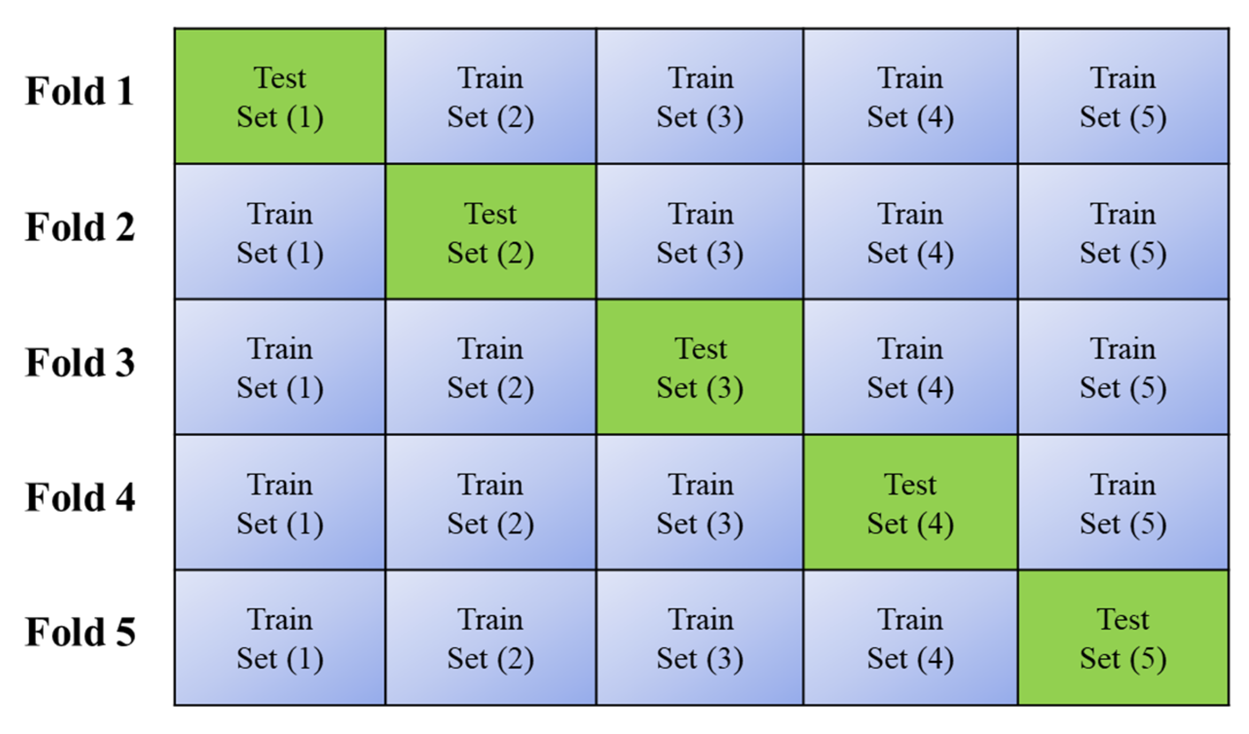
| Training Protocol | Five-fold cross-validation |
| Parameters (Mean of Five Trails) | Mathematical Expression |
|---|---|
| Mean Accuracy | |
| Mean Sensitivity | |
| Mean Specificity | |
| Mean Positive Predicted Value | |
| Mean Negative Predicted Value | |
| Mean Areas Under the Curve |
| Models | ||||||
|---|---|---|---|---|---|---|
| Mean ± SD | Mean ± SD | Mean ± SD | Mean ± SD | Mean ± SD | Mean ± SD | |
| AlexNet | 90.98 ± 2.90 | 90.91 ± 3.01 | 91.11 ± 3.04 | 91.01 ± 2.89 | 94.58 ± 1.88 | 85.50 ± 4.47 |
| VGG16 | 91.39 ± 2.54 | 91.69 ± 2.73 | 90.89 ± 3.08 | 91.29 ± 2.57 | 94.51 ± 1.83 | 86.56 ± 4.17 |
| ResNet18 | 92.79 ± 1.22 | 92.86 ± 1.03 | 92.67 ± 2.17 | 92.76 ± 1.37 | 95.60 ± 1.26 | 88.35 ± 1.58 |
| GoogleNet | 88.61 ± 1.62 | 89.48 ± 1.41 | 87.11 ± 2.43 | 88.30 ± 1.76 | 92.24 ± 1.42 | 82.88 ± 2.18 |
| ResNet50 | 93.85 ± 1.71 | 94.03 ± 1.48 | 93.56 ± 2.28 | 93.79 ± 1.82 | 96.15 ± 1.36 | 90.16 ± 2.40 |
| MajVot Algorithm | 94.75 ± 0.61 | 94.29 ± 0.54 | 95.56 ± 0.79 | 94.92 ± 0.64 | 97.32 ± 0.47 | 90.72 ± 0.86 |
| Models | ||||||
|---|---|---|---|---|---|---|
| Mean ± SD | Mean ± SD | Mean ± SD | Mean ± SD | Mean ± SD | Mean ± SD | |
| AlexNet | 94.35 ± 0.75 | 94.56 ± 1.19 | 94.15 ± 0.68 | 94.35 ± 0.75 | 94.26 ± 0.65 | 94.46 ± 1.15 |
| VGG16 | 94.76 ± 2.53 | 94.24 ± 3.01 | 95.28 ± 2.10 | 94.76 ± 2.53 | 95.29 ± 2.15 | 94.24 ± 2.95 |
| ResNet18 | 96.45 ± 0.60 | 96.00 ± 0.57 | 96.91 ± 0.68 | 96.46 ± 0.60 | 96.93 ± 0.67 | 95.97 ± 0.57 |
| GoogleNet | 94.76 ± 1.48 | 94.40 ± 1.70 | 95.12 ± 1.29 | 94.76 ± 1.48 | 95.16 ± 1.30 | 94.36 ± 1.68 |
| ResNet50 | 96.69 ± 0.53 | 96.64 ± 0.67 | 96.75 ± 0.57 | 96.69 ± 0.53 | 96.80 ± 0.56 | 96.59 ± 0.67 |
| MajVot Algorithm | 97.98 ± 0.86 | 97.60 ± 0.98 | 98.37 ± 0.81 | 97.99 ± 0.85 | 98.39 ± 0.81 | 97.58 ± 0.97 |
| Models | ||||||
|---|---|---|---|---|---|---|
| Mean ± SD | Mean ± SD | Mean ± SD | Mean ± SD | Mean ± SD | Mean ± SD | |
| AlexNet | 95.80 ± 1.19 | 95.29 ± 1.26 | 96.39 ± 1.45 | 95.84 ± 1.19 | 96.82 ± 1.26 | 94.69 ± 1.40 |
| VGG16 | 97.20 ± 0.65 | 97.39 ± 0.46 | 96.99 ± 0.92 | 97.19 ± 0.67 | 97.39 ± 0.79 | 96.99 ± 0.54 |
| ResNet18 | 97.62 ± 0.63 | 97.52 ± 0.85 | 97.74 ± 0.53 | 97.63 ± 0.61 | 98.03 ± 0.46 | 97.17 ± 0.95 |
| GoogleNet | 95.80 ± 0.93 | 95.69 ± 0.75 | 95.94 ± 1.14 | 95.81 ± 0.94 | 96.44 ± 0.99 | 95.08 ± 0.86 |
| ResNet50 | 97.76 ± 0.59 | 97.91 ± 0.55 | 97.59 ± 0.63 | 97.75 ± 0.59 | 97.91 ± 0.55 | 97.59 ± 0.63 |
| MajVot Algorithm | 98.88 ± 0.63 | 98.95 ± 0.58 | 98.80 ± 0.67 | 98.88 ± 0.63 | 98.95 ± 0.58 | 98.80 ± 0.67 |
| DataSet | ACC | SEN | SPC | AUC | PPV | NPV |
|---|---|---|---|---|---|---|
| Mean ± SD | Mean ± SD | Mean ± SD | Mean ± SD | Mean ± SD | Mean ± SD | |
| T1W-MRI | 94.75 ± 0.61 | 94.29 ± 0.54 | 95.56 ± 0.79 | 94.92 ± 0.64 | 97.32 ± 0.47 | 90.72 ± 0.86 |
| T2W-MRI | 97.98 ± 0.86 | 97.60 ± 0.98 | 98.37 ± 0.81 | 97.99 ± 0.85 | 98.39 ± 0.81 | 97.58 ± 0.97 |
| FLAIR-MRI | 98.88 ± 0.63 | 98.95 ± 0.58 | 98.80 ± 0.67 | 98.88 ± 0.63 | 98.95 ± 0.58 | 98.80 ± 0.67 |
| IMP (%) of FLAIR-MRI Data | ACC | SEN | SPC | AUC | PPV | NPV |
|---|---|---|---|---|---|---|
| T1W-MRI Data | 4.17% | 4.72 | 3.28 | 4.00 | 1.65 | 8.18 |
| T2W-MRI Data | 0.91% | 1.37 | 0.43 | 0.90 | 0.57 | 1.23 |
| Model | T1W-MRI | T2W-MRI | FLAIR-MRI |
|---|---|---|---|
| AlexNet | 90.98 | 94.35 | 95.80 |
| VGG16 | 91.39 | 94.76 | 97.20 |
| ResNet18 | 92.79 | 96.45 | 97.62 |
| GoogleNet | 88.61 | 94.76 | 95.80 |
| ResNet50 | 93.85 | 96.69 | 97.76 |
| MajVot-Algorithm | 94.75 | 97.98 | 98.88 |
| Dataset | ACC | SEN | SPC | AUC | PPV | NPV |
|---|---|---|---|---|---|---|
| T1W-MRI | 92.06 ± 2.02 | 92.21 ± 1.70 | 91.81 ± 2.62 | 92.01 ± 2.14 | 95.07 ± 1.58 | 87.36 ± 2.72 |
| T2W-MRI | 95.83 ± 1.31 | 95.57 ± 1.27 | 96.10 ± 1.40 | 95.84 ± 1.31 | 96.14 ± 1.37 | 95.54 ± 1.27 |
| FLAIR-MRI | 97.18 ± 1.10 | 97.12 ± 1.27 | 97.24 ± 0.94 | 97.18 ± 1.08 | 97.59 ± 0.83 | 96.72 ± 1.42 |
| Model | ACC | SEN | SPC | AUC | PPV | NPV |
|---|---|---|---|---|---|---|
| AlexNet | 93.71 ± 2.47 | 93.59 ± 2.35 | 93.88 ± 2.65 | 93.74 ± 2.47 | 95.22 ± 1.39 | 91.55 ± 5.24 |
| VGG16 | 94.45 ± 2.92 | 94.44 ± 2.85 | 94.39 ± 3.15 | 94.41 ± 2.97 | 95.73 ± 1.49 | 92.59 ± 5.41 |
| ResNet18 | 95.62 ± 2.52 | 95.46 ± 2.38 | 95.77 ± 2.72 | 95.62 ± 2.54 | 96.85 ± 1.22 | 93.83 ± 4.78 |
| GoogleNet | 93.06 ± 3.89 | 93.19 ± 3.28 | 92.72 ± 4.88 | 92.96 ± 4.07 | 94.61 ± 2.15 | 90.78 ± 6.84 |
| ResNet50 | 96.10 ± 2.02 | 96.19 ± 1.98 | 95.97 ± 2.13 | 96.08 ± 2.05 | 96.95 ± 0.89 | 94.78 ± 4.03 |
| MajVot Algorithm | 97.21 ± 2.17 | 96.95 ± 2.40 | 97.58 ± 1.76 | 97.26 ± 2.08 | 98.22 ± 0.83 | 95.70 ± 4.36 |
| SN | Reference | Data Source | Class | MRI-Sequence | Preprocessing | Model | CV | Highest Accuracy (%) |
|---|---|---|---|---|---|---|---|---|
| 1 | Yang et al. [69] | TCIA (REMBRANDT) | 2 | T1W | ROI | AlexNet and GoogleNet | K5 | 94.5% |
| 2 | Khawaldeh et al. [79] | TCIA (REMBRANDT) | 3 | FLAIR | Whole image | Modified AlexNet | NA | 91.16% |
| 3 | Alies et al. [78] | NA | 2 | T1W-c T2W FLAIR | ROI/Whole image | ANN | NA | 88.3% |
| 4 | Anaraki et al. [80] | TCIA (REMBRANDT) and Others | 3/4 | T1W | ROI Segmented | Proposed CNN | NA | 94.2% |
| 5 | Swati et al. [81] | Figshar Data | 3 | T1W | Whole image | VGG19 | K5 | 94.82% |
| 6 | Badža et al. [82] | Tianjin Medical University, China | 3 | T1W | Whole image | Proposed CNN | K10 | 96.56% |
| 7 | Our method | TCIA (REMBRANDT) | 2 | T1W T2W FLAIR | Whole image | MajVot (AlexNet, VGG16, ResNet18, GoogleNet, ResNet50) | K5 | FLAIR-MRI (98.88%) T2W-MRI (97.98%) T1W-MRI (94.75%) |
Disclaimer/Publisher’s Note: The statements, opinions and data contained in all publications are solely those of the individual author(s) and contributor(s) and not of MDPI and/or the editor(s). MDPI and/or the editor(s) disclaim responsibility for any injury to people or property resulting from any ideas, methods, instructions or products referred to in the content. |
© 2023 by the authors. Licensee MDPI, Basel, Switzerland. This article is an open access article distributed under the terms and conditions of the Creative Commons Attribution (CC BY) license (https://creativecommons.org/licenses/by/4.0/).
Share and Cite
Tandel, G.S.; Tiwari, A.; Kakde, O.G.; Gupta, N.; Saba, L.; Suri, J.S. Role of Ensemble Deep Learning for Brain Tumor Classification in Multiple Magnetic Resonance Imaging Sequence Data. Diagnostics 2023, 13, 481. https://doi.org/10.3390/diagnostics13030481
Tandel GS, Tiwari A, Kakde OG, Gupta N, Saba L, Suri JS. Role of Ensemble Deep Learning for Brain Tumor Classification in Multiple Magnetic Resonance Imaging Sequence Data. Diagnostics. 2023; 13(3):481. https://doi.org/10.3390/diagnostics13030481
Chicago/Turabian StyleTandel, Gopal S., Ashish Tiwari, Omprakash G. Kakde, Neha Gupta, Luca Saba, and Jasjit S. Suri. 2023. "Role of Ensemble Deep Learning for Brain Tumor Classification in Multiple Magnetic Resonance Imaging Sequence Data" Diagnostics 13, no. 3: 481. https://doi.org/10.3390/diagnostics13030481