
Classification of Atypical White Blood Cells in Acute Myeloid Leukemia Using a Two-Stage Hybrid Model Based on Deep Convolutional Autoencoder and Deep Convolutional Neural Network

 and
and
Abstract
:1. Introduction
- A new WBC augmentation model called “the GT-DCAE WBC augmentation model” is developed by combining a geometric transformation model and a generative model by using deep convolutional autoencoder.
- A new model for classifying atypical white blood cells (WBCs) that includes immature WBCs and atypical lymphocytes is created. This model is called “the Two-stage DCAE-CNN atypical WBC classification model”, and it uses a combination of a deep convolutional autoencoder and a convolutional neural network.
- The newly proposed model is a context-free generalized model that incorporates only features associated with WBCs and excludes other blood components.
2. Related Work
3. Materials and Methods
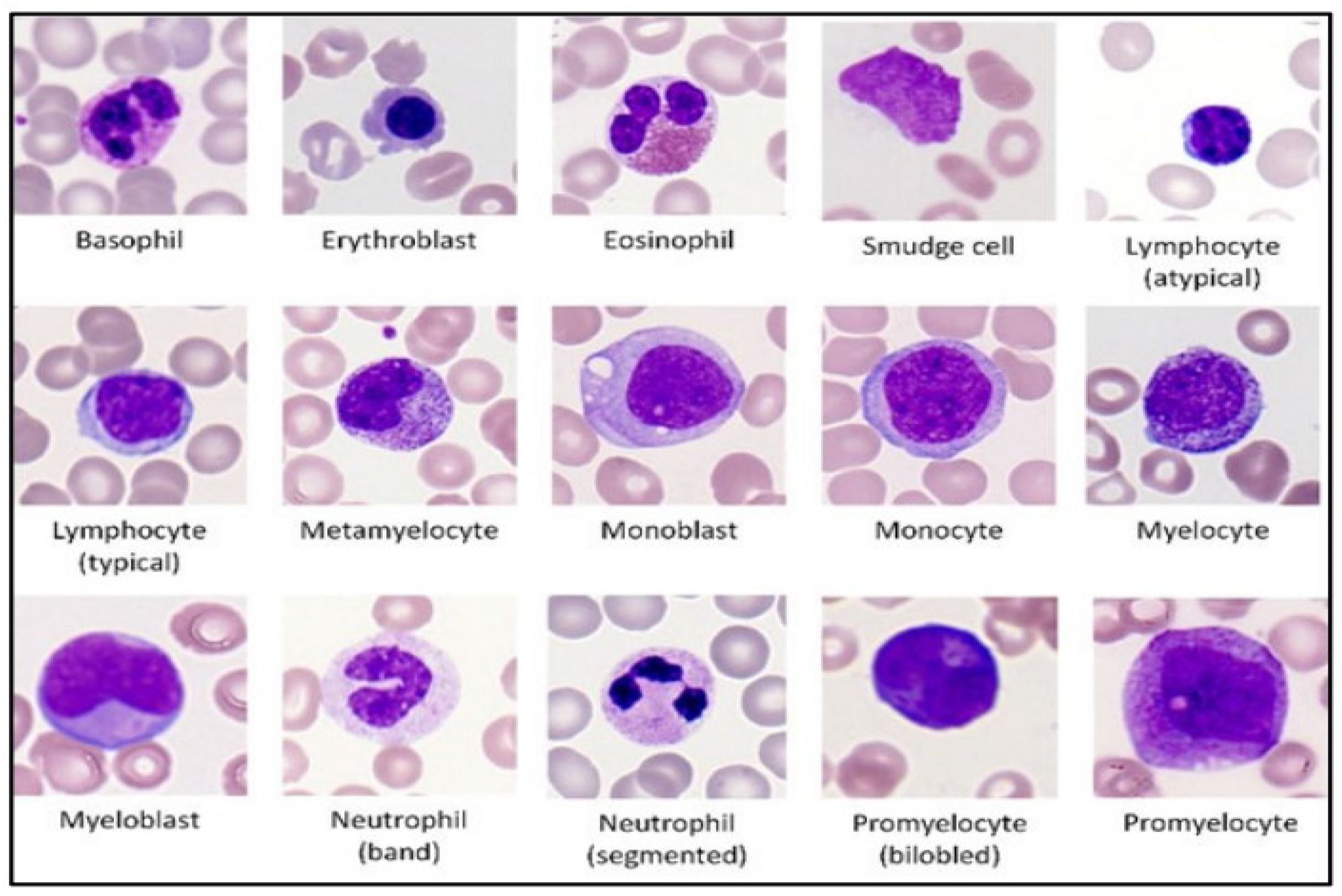
3.1. Dataset
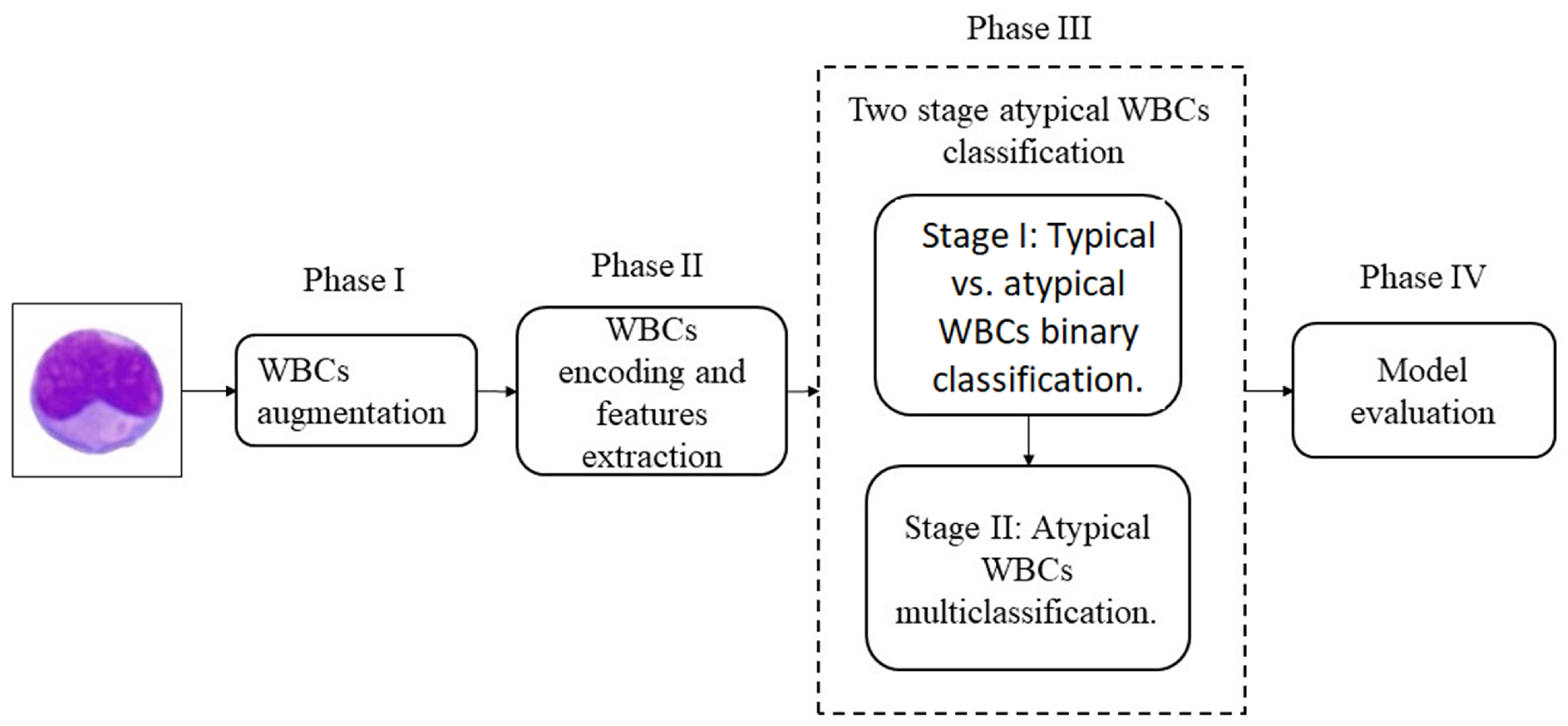
3.2. The Proposed Model
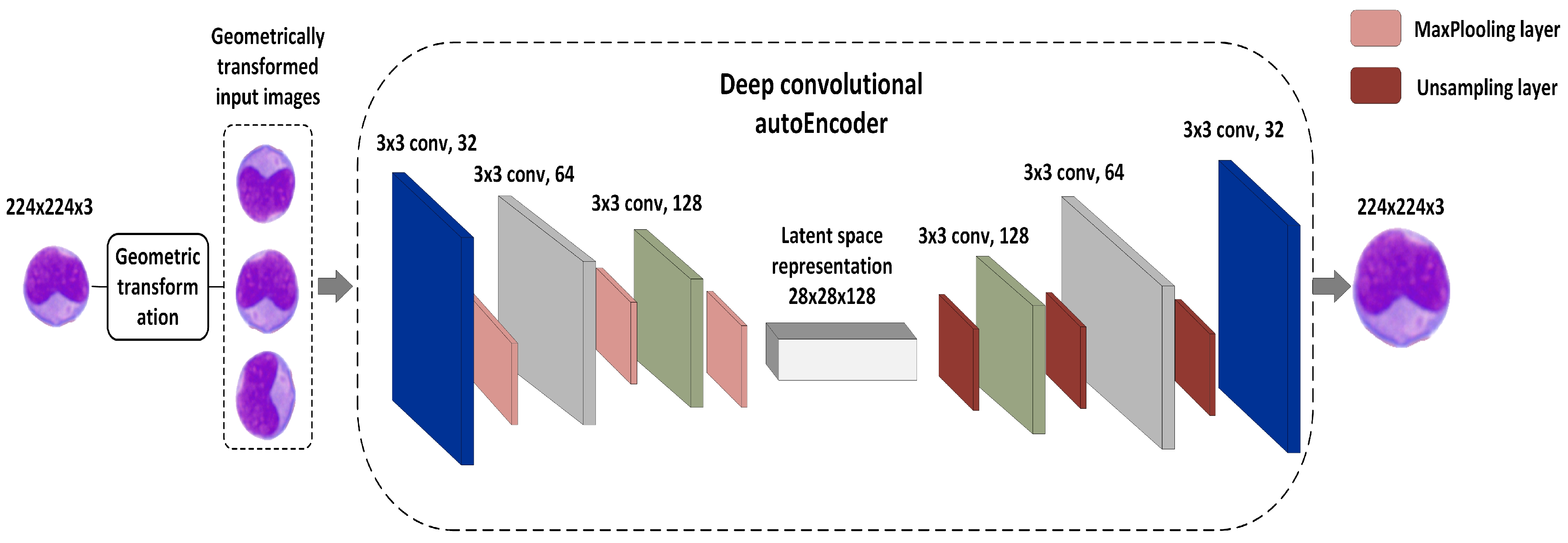
3.2.1. Phase I: WBC Augmentation
- The encoder network: Using filter banks, the encoder network performed several convolutional operations to generate a new set of feature maps. The encoder network comprised three convolutional layers of 32, 64, and 128 filters using a 3 × 3 kernel and a LeakyReLU activation function. Following every convolutional layer was a maximum pooling layer of size 2 × 2 and a one-step stride. This method yielded a collection of pooled feature maps with the greatest weights. In this situation, the maximum pooling layer could be viewed as a feature selection strategy analogous to the feature selection algorithms used in conventional ML approaches.
- Latent vector space: This was expressed as 28 × 28 × 128, with 28 × 28 being the image size and 128 representing the number of compressed feature mappings. To retain the semantics across the encoder and decoder units, we built a latent vector space by using convolutional layers as opposed to dense layers [22]. The latent vector could be obtained by using the following equation:where Z denotes the latent vector, X is the WBC input image, and W and b are the weights and bias, respectively. denotes the activation function.
- The decoder network: This consisted of three convolutional layers of 128, 64, and 32 filters using a 3 × 3 kernel and a LeakyReLU activation function. To reconstruct the compressed image into the original, each convolutional layer was up-sampled by using a subsampling layer. The reconstruction process of the encoded image shown in Equation (1) can be expresses as follows:where identifies the inverse operation across both weight dimensions of the kth feature map. C denotes the bias. Algorithm 1 shows the details of the GT-DCAE augmentation model.
| Algorithm 1 The GT-DCAE WBC augmentation algorithm. |
|
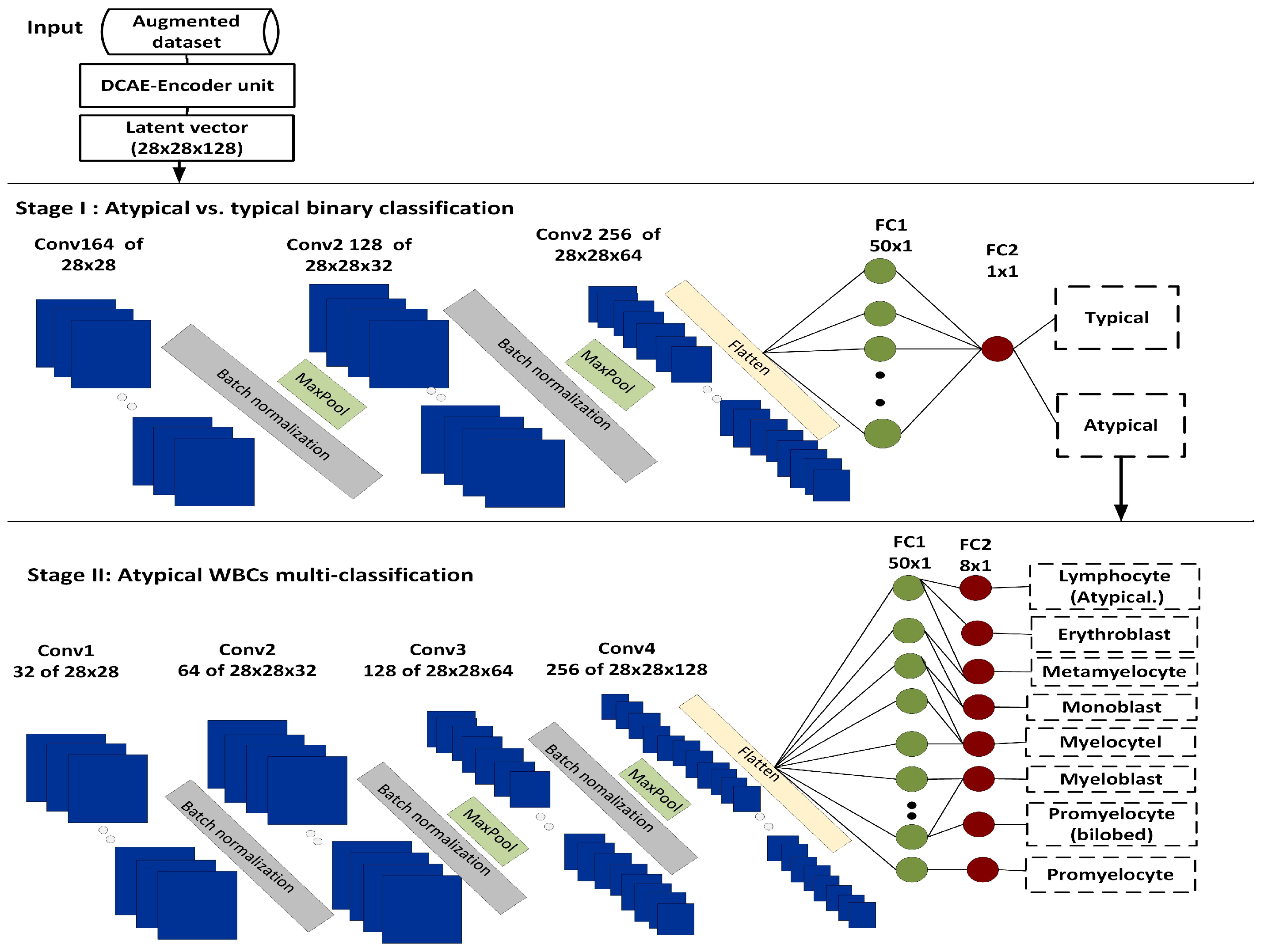
3.2.2. Phase II: WBC Encoding and Feature Extraction
3.2.3. Phase III: The Two-Stage Atypical WBC Classification
| Algorithm 2 The two-Stage DCAE-CNN atypical WBC classification algorithm. |
|
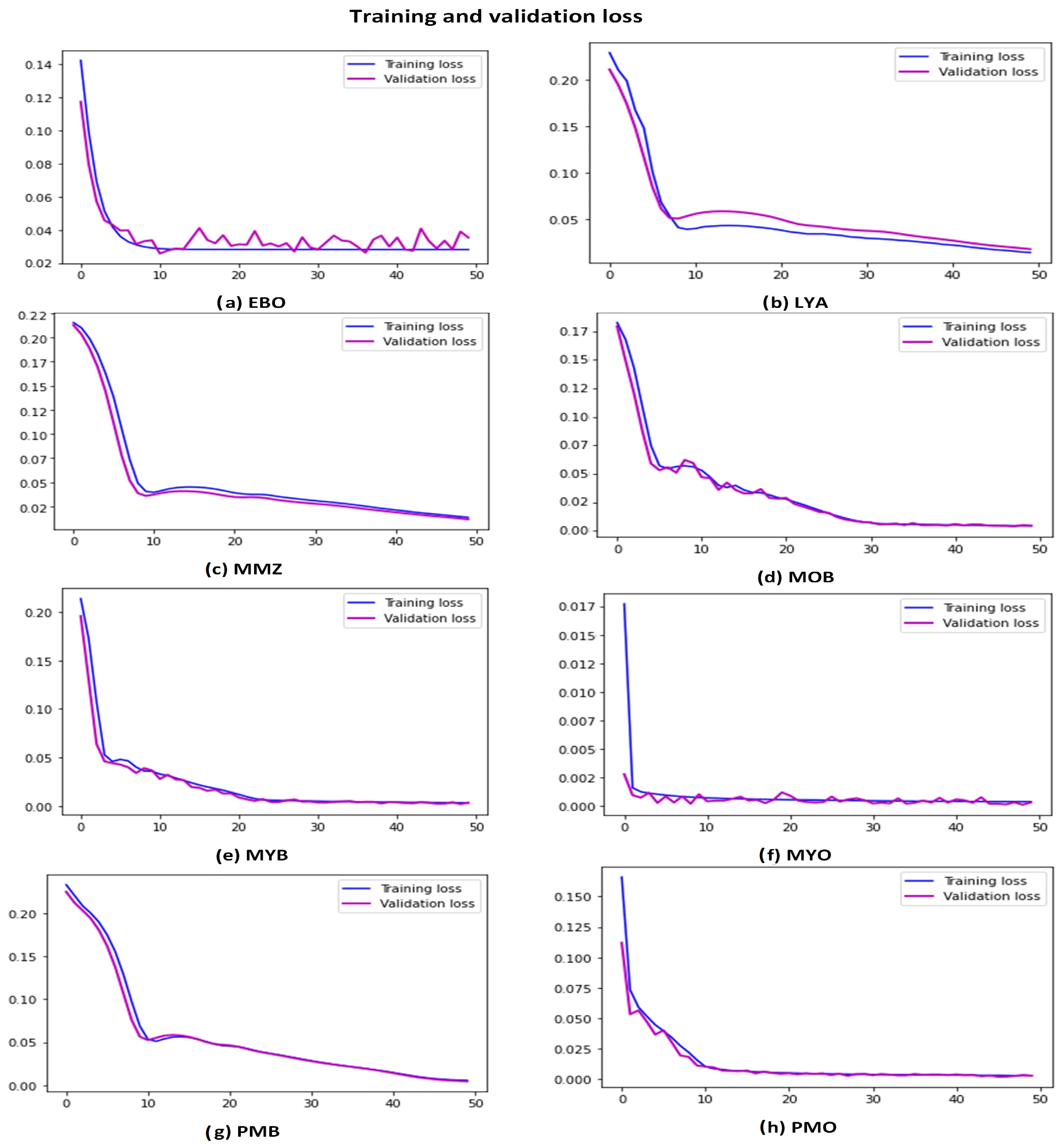
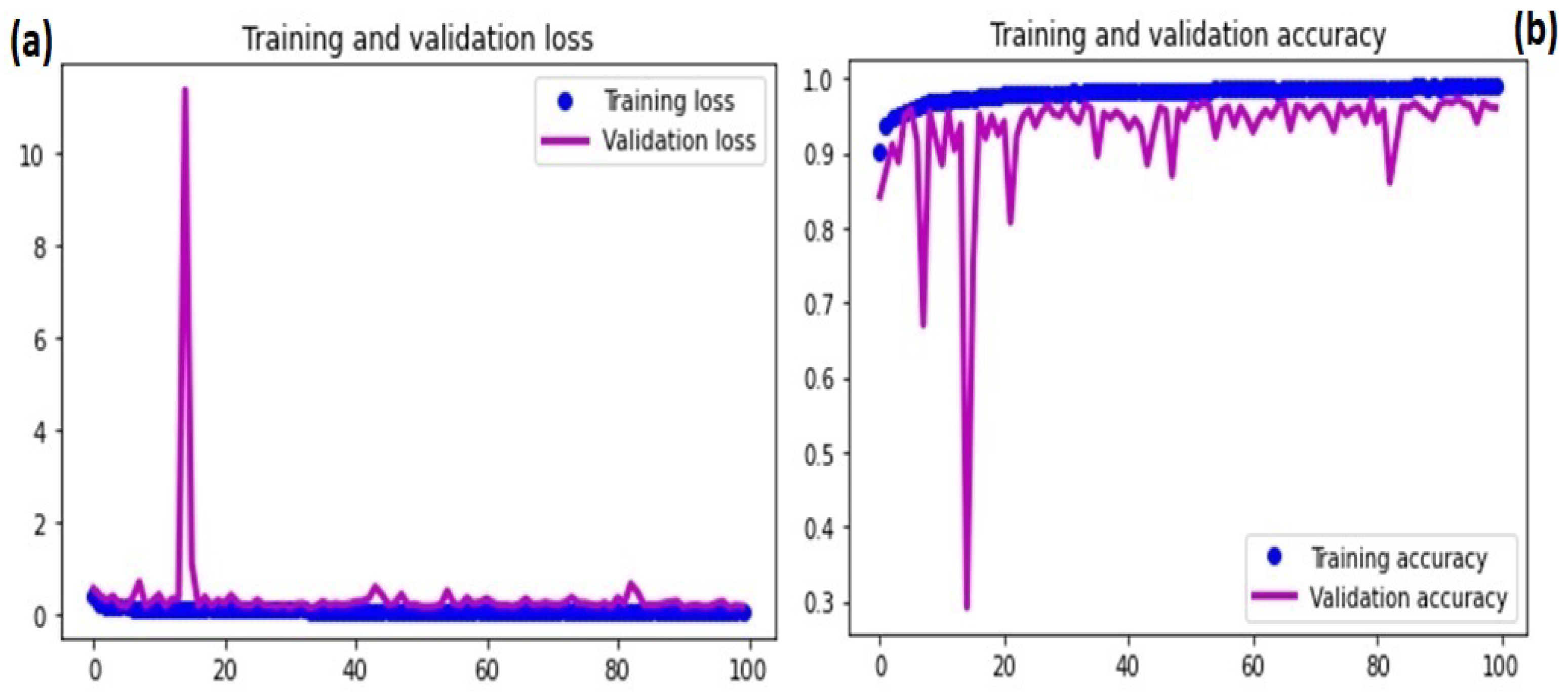
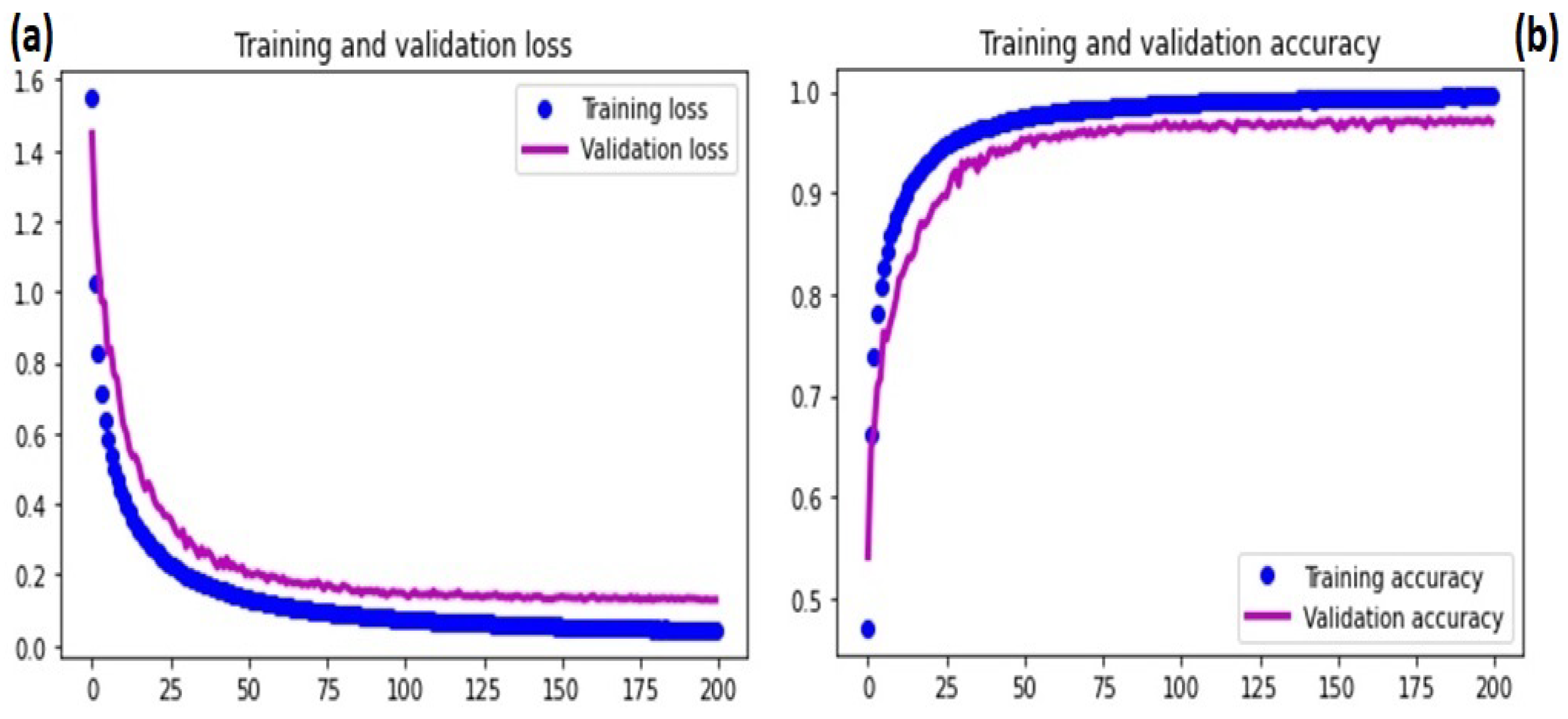
3.2.4. Model Training
3.2.5. Phase III: Model Evaluation
4. Results
4.1. WBC Augmentation
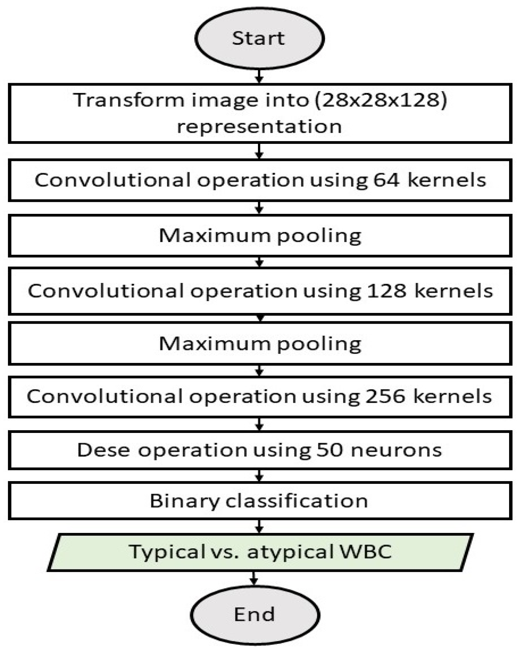
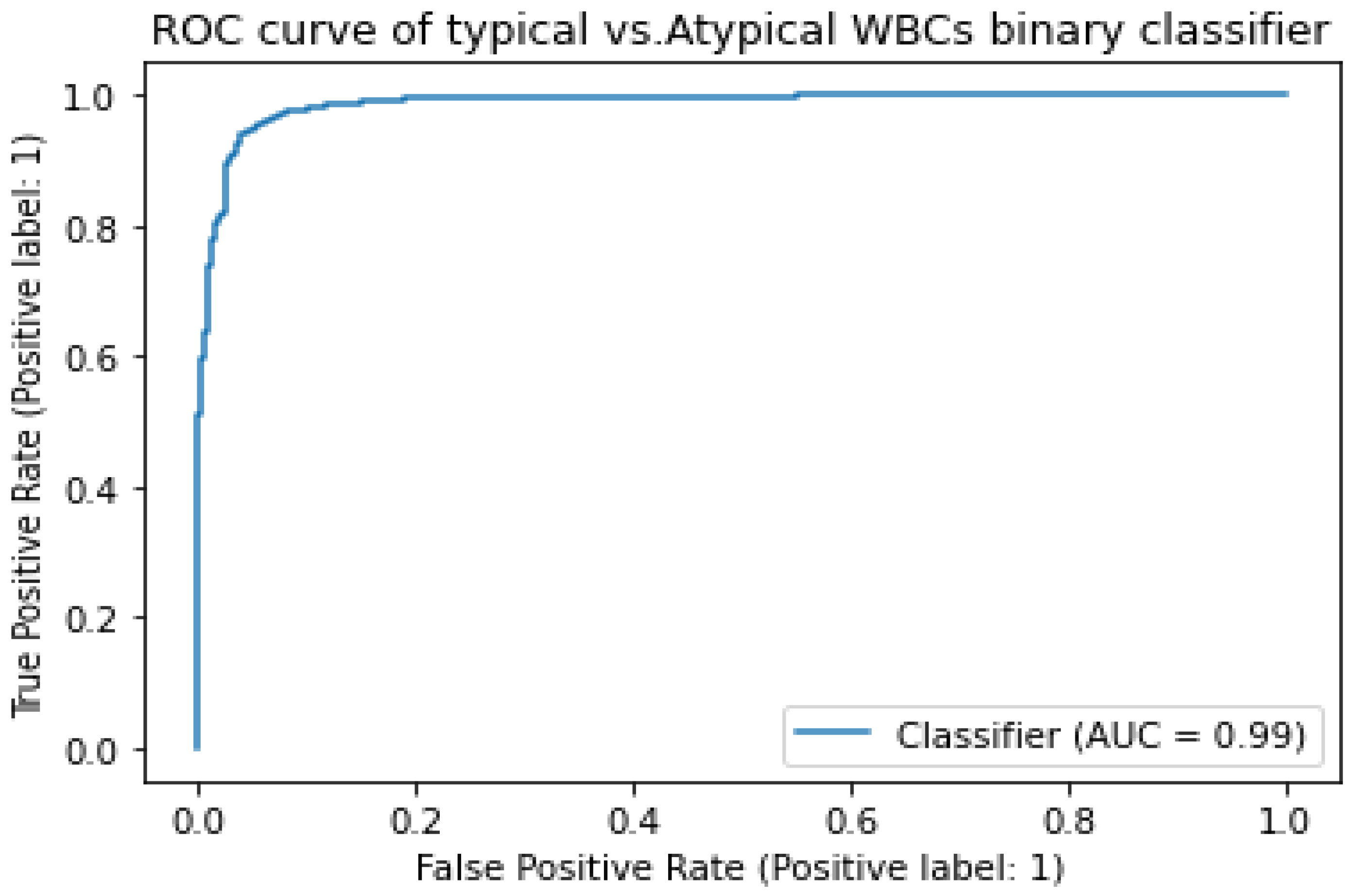
4.2. Stage 1: Typical vs. Atypical Binary Classification
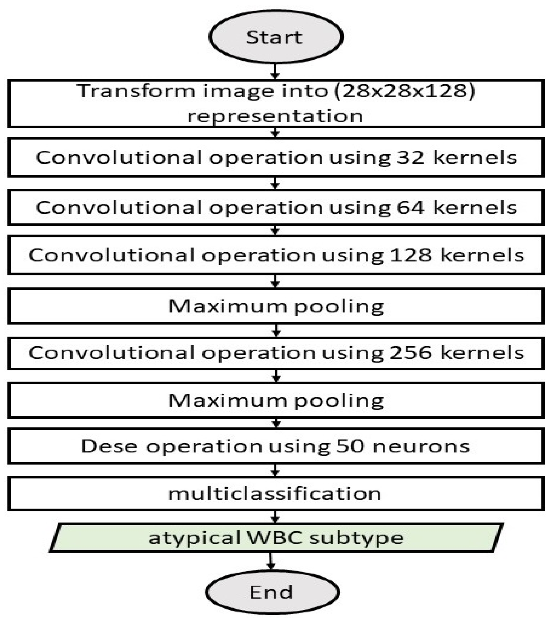
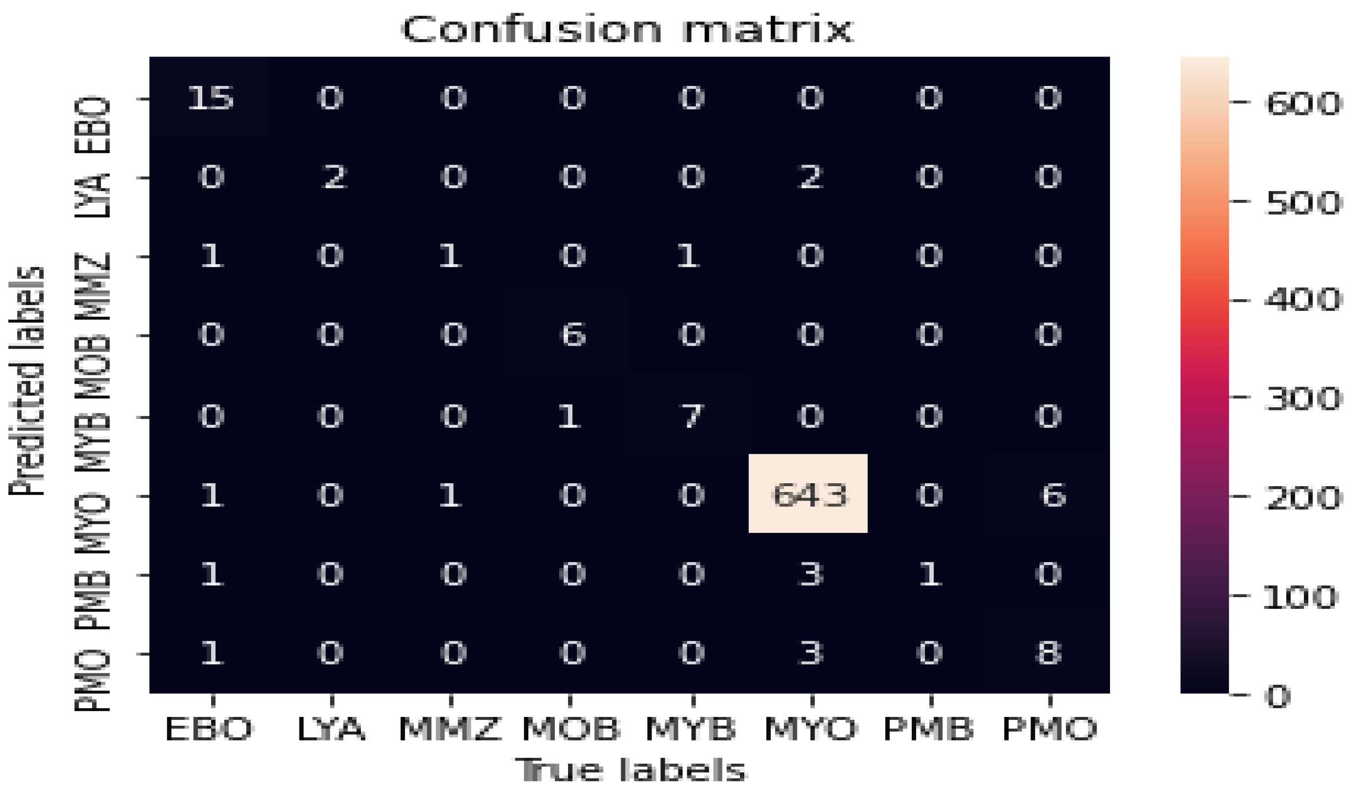
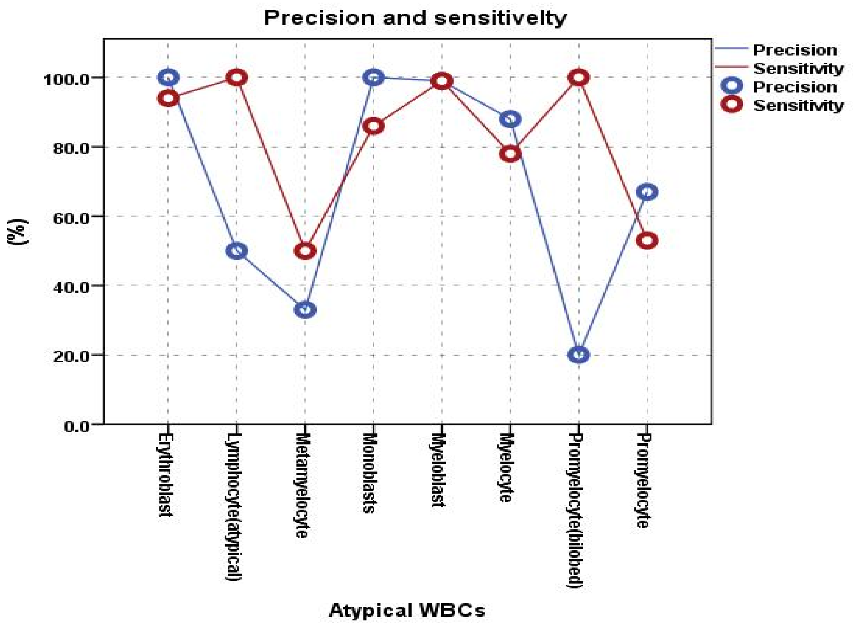
4.3. Stage II: The Atypical WBC Multiclassification Model
- CNN model employing GT-DCAE images without features extracted by the DCAE to evaluate the significance of the DCAE-extracted features, as shown in Table 3.
- DCAE-CNN on GT images, excluding synthetic images generated by the DCAE model, to examine the impact of synthetic images on improving the classification accuracy, as presented in Table 4.
5. Conclusions
Author Contributions
Funding
Institutional Review Board Statement
Informed Consent Statement
Data Availability Statement
Conflicts of Interest
References
- Walker, H.K.; Hall, W.D.; Hurst, J.W. Clinical methods: The history, physical, and laboratory examinations. JAMA 1990, 264, 2808–2809. [Google Scholar]
- Matek, C.; Schwarz, S.; Spiekermann, K.; Marr, C. Human-level recognition of blast cells in acute myeloid leukaemia with convolutional neural networks. Nat. Mach. Intell. 2019, 1, 538–544. [Google Scholar] [CrossRef]
- Krappe, S.; Wittenberg, T.; Haferlach, T.; Münzenmayer, C. Automated morphological analysis of bone marrow cells in microscopic images for diagnosis of leukemia: Nucleus-plasma separation and cell classification using a hierarchical tree model of hematopoesis. In Proceedings of the Medical Imaging 2016: Computer-Aided Diagnosis, San Diego, CA, USA, 24 March 2016; SPIE: Bellingham, WA, USA, 2016; Volume 9785, pp. 856–861. [Google Scholar]
- Al-Dulaimi, K.A.K.; Banks, J.; Chandran, V.; Tomeo-Reyes, I.; Nguyen Thanh, K. Classification of white blood cell types from microscope images: Techniques and challenges. Microsc. Sci. 2018, 8, 17–25. [Google Scholar]
- Dinčić, M.; Popović, T.B.; Kojadinović, M.; Trbovich, A.M.; Ilić, A.Ž. Morphological, fractal, and textural features for the blood cell classification: The case of acute myeloid leukemia. Eur. Biophys. J. 2021, 50, 1111–1127. [Google Scholar] [CrossRef] [PubMed]
- Choi, J.W.; Ku, Y.; Yoo, B.W.; Kim, J.A.; Lee, D.S.; Chai, Y.J.; Kong, H.J.; Kim, H.C. White blood cell differential count of maturation stages in bone marrow smear using dual-stage convolutional neural networks. PLoS ONE 2017, 12, e0189259. [Google Scholar] [CrossRef] [PubMed] [Green Version]
- Elhassan, T.A.M.; Rahim, M.S.M.; Swee, T.T.; Hashim, S.Z.M.; Aljurf, M. Feature Extraction of White Blood Cells Using CMYK-Moment Localization and Deep Learning in Acute Myeloid Leukemia Blood Smear Microscopic Images. IEEE Access 2022, 10, 16577–16591. [Google Scholar] [CrossRef]
- Bigorra, L.; Merino, A.; Alferez, S.; Rodellar, J. Feature analysis and automatic identification of leukemic lineage blast cells and reactive lymphoid cells from peripheral blood cell images. J. Clin. Lab. Anal. 2017, 31, e22024. [Google Scholar] [CrossRef] [PubMed]
- Rad, A.E.; Rahim, M.S.M.; Rehman, A.; Saba, T. Digital dental X-ray database for caries screening. 3D Res. 2016, 7, 1–5. [Google Scholar] [CrossRef]
- Rad, A.E.; Mohd Rahim, M.S.; Kolivand, H.; Mat Amin, I.B. Morphological region-based initial contour algorithm for level set methods in image segmentation. Multimed. Tools Appl. 2017, 76, 2185–2201. [Google Scholar] [CrossRef] [Green Version]
- Muhsen, I.N.; Elhassan, T.; Hashmi, S.K. Artificial intelligence approaches in hematopoietic cell transplantation: A review of the current status and future directions. Turk. J. Hematol. 2018, 35, 152. [Google Scholar]
- Elhassan, T.A.; Rahim, M.S.M.; Swee, T.T.; Hashim, S.Z.M.; Aljurf, M. Segmentation of White Blood Cells in Acute Myeloid Leukemia Microscopic Images: A Review. In Prognostic Models in Healthcare: AI and Statistical Approaches; Springer: Berlin/Heidelberg, Germany, 2022; pp. 1–24. [Google Scholar]
- Suryani, E.; Wiharto, W.; Polvonov, N. Identification and counting white blood cells and red blood cells using image processing case study of leukemia. arXiv 2015, arXiv:1511.04934. [Google Scholar]
- Wiharto, E.S.; Palgunadi, S.; Putra, Y.R.; Suryani, E. Cells identification of acute myeloid leukemia AML M0 and AML M1 using K-nearest neighbour based on morphological images. In Proceedings of the 2017 International Conference on Data and Software Engineering (ICoDSE), Palembang, Indonesia, 1–2 November 2017; IEEE: Piscataway, NJ, USA, 2017; pp. 1–6. [Google Scholar]
- Wiharto, W.; Suryani, E.; Putra, Y.R. Classification of blast cell type on acute myeloid leukemia (AML) based on image morphology of white blood cells. Telecommun. Comput. Electron. Control 2019, 17, 645–652. [Google Scholar] [CrossRef] [Green Version]
- Harjoko, A.; Ratnaningsih, T.; Suryani, E.; Palgunadi, S.; Prakisya, N.P.T. Classification of acute myeloid leukemia subtypes M1, M2 and M3 using active contour without edge segmentation and momentum backpropagation artificial neural network. In Proceedings of the MATEC Web of Conferences, Bandung, Indonesia, 18 April 2018; EDP Sciences: Les Ulis, France, 2018; Volume 154, p. 01041. [Google Scholar]
- Roy, E.K.; Aditya, S.K. Prediction of acute myeloid leukemia subtypes based on artificial neural network and adaptive neuro-fuzzy inference system approaches. In Innovations in Electronics and Communication Engineering; Springer: Berlin/Heidelberg, Germany, 2019; pp. 427–439. [Google Scholar]
- Rawat, J.; Singh, A.; Bhadauria, H.; Virmani, J.; Devgun, J.S. Computer assisted classification framework for prediction of acute lymphoblastic and acute myeloblastic leukemia. Biocybern. Biomed. Eng. 2017, 37, 637–654. [Google Scholar] [CrossRef]
- Dasariraju, S.; Huo, M.; McCalla, S. Detection and classification of immature leukocytes for diagnosis of acute myeloid leukemia using random forest algorithm. Bioengineering 2020, 7, 120. [Google Scholar] [CrossRef] [PubMed]
- Qin, F.; Gao, N.; Peng, Y.; Wu, Z.; Shen, S.; Grudtsin, A. Fine-grained leukocyte classification with deep residual learning for microscopic images. Comput. Methods Programs Biomed. 2018, 162, 243–252. [Google Scholar] [CrossRef] [PubMed]
- Matek, C.; Schwarz, S.; Marr, C.; Spiekermann, K. A Single-Cell Morphological Dataset of Leukocytes from AML Patients and Non-Malignant Controls [Data Set]; The Cancer Imaging Archive: Frederick, MD, USA, 2019. [Google Scholar]
- Trang, K.; TonThat, L.; Thao, N.G.M. Plant leaf disease identification by deep convolutional autoencoder as a feature extraction approach. In Proceedings of the 2020 17th International Conference on Electrical Engineering/Electronics, Computer, Telecommunications and Information Technology (ECTI-CON), Phuket, Thailand, 24–27 June 2020; IEEE: Piscataway, NJ, USA, 2020; pp. 522–526. [Google Scholar]
- He, G.; Wang, C.; Li, Q.; Tan, H.; Chen, F.; Huang, Z.; Yu, B.; Zheng, L.; Zheng, R.; Liu, D. Clinical and laboratory features of seven patients with acute myeloid leukemia (AML)-M2/M3 and elevated myeloblasts and abnormal promyelocytes. Cancer Cell Int. 2014, 14, 1–9. [Google Scholar] [CrossRef] [PubMed] [Green Version]
- Almezhghwi, K.; Serte, S. Improved classification of white blood cells with the generative adversarial network and deep convolutional neural network. Comput. Intell. Neurosci. 2020, 2020, 6490479. [Google Scholar] [CrossRef] [PubMed]
- Bradshaw, R.A.; Stahl, P.D. Encyclopedia of Cell Biology; Academic Press: Cambridge, MA, USA, 2015. [Google Scholar]


| Precision | Sensitivity | Number of Images/Class | |
|---|---|---|---|
| Erythroblast | 1.00 | 0.94 | 78. |
| Lymphocyte (atypical) | 0.50 | 1.00 | 11 |
| Metamyelocyte | 0.33 | 0.50 | 15 |
| Monoblast | 1.00 | 0.86 | 26 |
| Myeloblast | 0.99 | 0.99 | 3268 |
| Myelocyte | 0.88 | 0.78 | 42 |
| Promyelocyte (bilobed) | 0.20 | 1.00 | 18 |
| Promyelocyte | 0.67 | 0.53 | 70 |
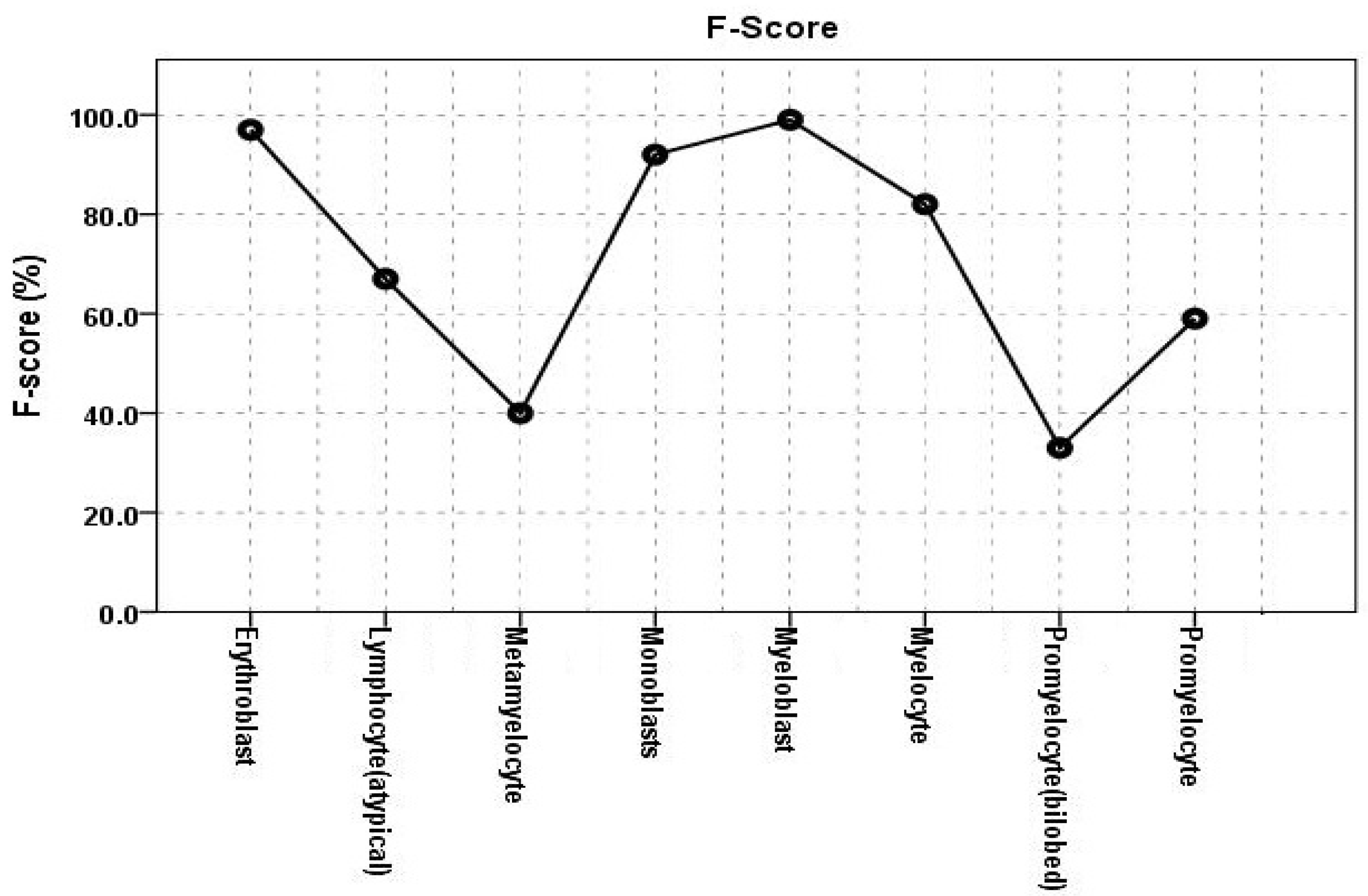
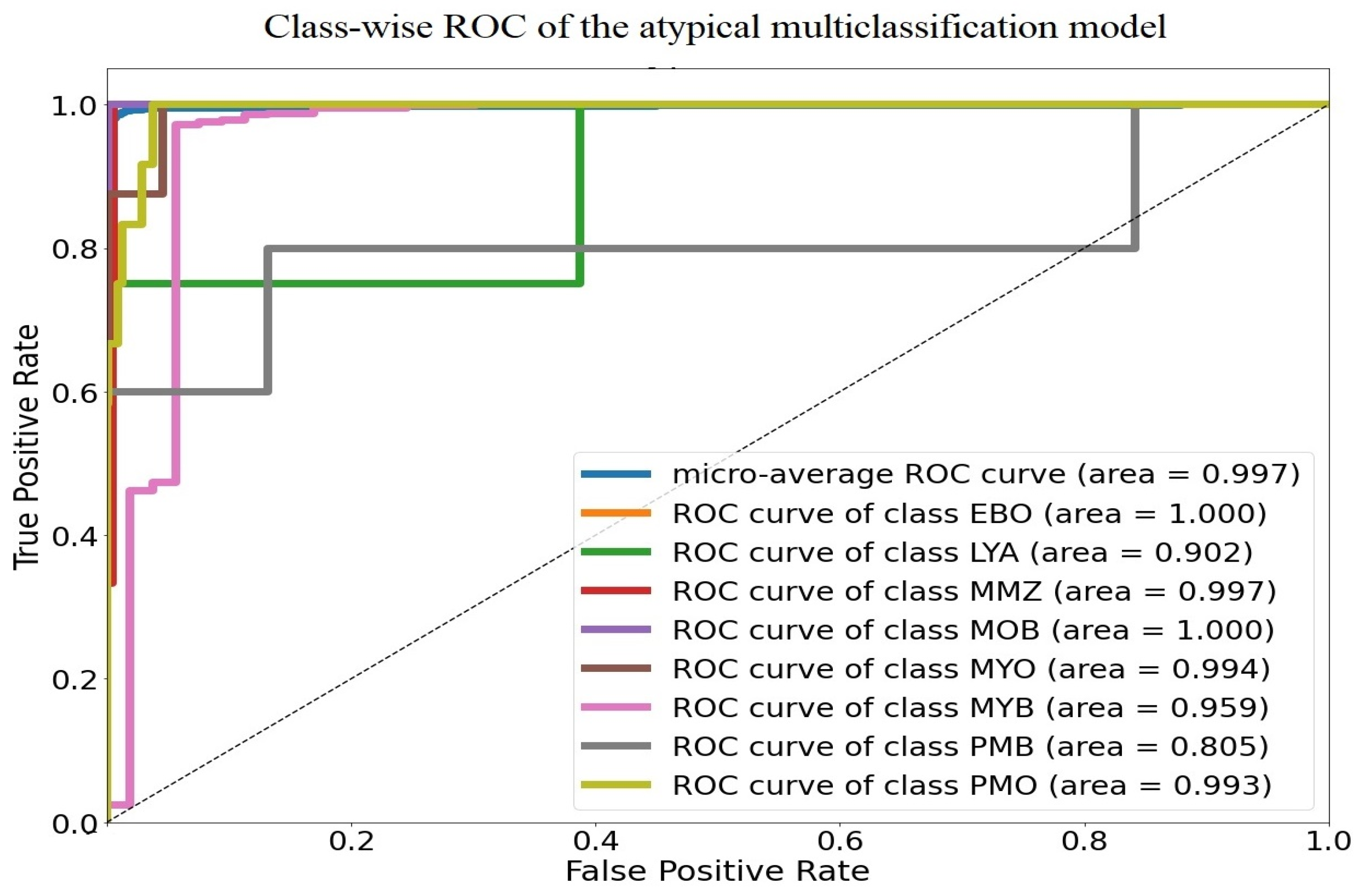
| WBCs | F-Score | AUC |
|---|---|---|
| Erythroblast | 0.9700 | 1.0000 |
| Lymphocyte (atypical) | 0.6700 | 0.9020 |
| Metamyelocyte | 0.4000 | 0.9970 |
| Monoblast | 0.9200 | 1.0000 |
| Myeloblast | 0.9900 | 0.9900 |
| Myelocyte | 0.8200 | 0.9590 |
| Promyelocyte (bilobed) | 0.3300 | 0.80500 |
| Promyelocyte | 0.5900 | 0.9930 |
| GT-DCAE | GT | |||
|---|---|---|---|---|
| Precision | Sensitivity | Precision | Sensitivity | |
| Erythroblast | 1.00 | 0.94 | 1.00 | 0.20 |
| Lymphocyte (atyp) | 5.00 | 1.00 | 0.00 | 0.00 |
| Metamyelocyte | 0.33 | 0.50 | 0.00 | 0.00 |
| Monoblast | 1.00 | 0.86 | 0.00 | 0.00 |
| Myeloblast | 0.99 | 0.99 | 0.93 | 0.90 |
| Myelocyte | 0.88 | .78 | 0.00 | 0.00 |
| Promyelocyte (bilobed) | 0.20 | 1.00 | 0.00 | 0.00 |
| Promyelocyte | 0.67 | 0.53 | 0.00 | 0.00 |
| Average overall accuracy | 0.970 | 0.83 | ||
| GT-DCAE | GT | |||
|---|---|---|---|---|
| Precision | Sensitivity | Precision | Sensitivity | |
| Erythroblast | 1.00 | 0.94 | 1.00 | 0.79 |
| Lymphocyte (atyp) | 5.00 | 1.00 | 0.50 | 1.00 |
| Metamyelocyte | 0.50 | 1.00 | 0.50 | 1.00 |
| Metamyelocyte | 0.33 | 0.50 | 0.33 | 0.33 |
| Monoblast | 1.0 | 0.86 | 1.00 | 0.75 |
| Myeloblast | 0.99 | 0.99 | 0.95 | 1.00 |
| Myelocyte | 0.88 | 0.78 | 0.75 | 0.26 |
| Promyelocyte (bilobed) | 0.20 | 1.00 | 0.80 | 0.20 |
| Promyelocyte | 0.67 | 0.53 | 0.42 | 0.56 |
| Promyelocyte | 0.67 | 0.53 | 0.42 | 0.56 |
| Average overall accuracy | 0.97 | 0.93 | ||
| Authors | Matek et al. (2019) [2] | Dasariraju et al. (2020) [19] | Dincic et al. (2021) [5] | Our Model 2022 | ||||||||
|---|---|---|---|---|---|---|---|---|---|---|---|---|
| Prob. | Unadjusted | Unadjusted | Adjusted | Unadjusted | Unadjusted | Adjusted | ||||||
| Metrics | Precision | Sensitivity | Precision | Sensitivity | Precision | Sensitivity | Precision | Sensitivity | Precision | Sensitivity | Precision | Sensitivity |
| Erythroblast | 0.7500 | 0.8700 | 1.0000 | 0.9130 | 0.9123 | 0.8710 | 0.8600 | 1.0000 | 1.0000 | 0.9400 | 0.9679 | 0.9303 |
| Lymphocyte (atyp) | 0.200 | 0.0700 | - | - | - | - | - | - | 0.5000 | 1.000 | 0.4839 | 0.9897 |
| Metamyelocyte | 0.070 | 0.1300 | - | - | - | - | 0.5000 | 0.4300 | 0.3300 | 0.5000 | 0.3194 | 0.4948 |
| Monoblast | 0.5200 | 0.5800 | 0.8750 | 1.0000 | 0.7982 | 0.9540 | 0.8800 | 0.9600 | 1.0000 | 0.8600 | 0.9679 | 0.8512 |
| Myeloblast | 0.9400 | 0.9400 | 0.9675 | 0.9444 | 0.8826 | 0.9009 | 0.8000 | 0.9600 | 0.9900 | 0.9900 | 0.9582 | 0.9798 |
| Myelocyte | 0.4600 | 0.4300 | - | - | - | - | 0.6500 | 0.5200 | 0.8800 | 0.7800 | 0.8517 | 0.7720 |
| Promyelocyte (bilobed) | 0.4500 | 0.4100 | - | - | - | - | - | - | 0.2000 | 1.0000 | 0.1935 | 0.9897 |
| Promyelocyte | 0.6300 | 0.5400 | 0.6250 | 0.8330 | 0.5701 | 0.5439 | 0.8900 | 0.7100 | 0.6700 | 0.5300 | 0.6484 | 0.5245 |
| Overall Accuracy | - | 0.9340 | 0.8676 | 0.8100 | 0.9700 | 0.9312 | ||||||
| AUC | 0.9860 | Not Cal | Not cal | Not cal | 0.997 | 0.9897 | ||||||
Disclaimer/Publisher’s Note: The statements, opinions and data contained in all publications are solely those of the individual author(s) and contributor(s) and not of MDPI and/or the editor(s). MDPI and/or the editor(s) disclaim responsibility for any injury to people or property resulting from any ideas, methods, instructions or products referred to in the content. |
© 2023 by the authors. Licensee MDPI, Basel, Switzerland. This article is an open access article distributed under the terms and conditions of the Creative Commons Attribution (CC BY) license (https://creativecommons.org/licenses/by/4.0/).
Share and Cite
Elhassan, T.A.; Mohd Rahim, M.S.; Siti Zaiton, M.H.; Swee, T.T.; Alhaj, T.A.; Ali, A.; Aljurf, M. Classification of Atypical White Blood Cells in Acute Myeloid Leukemia Using a Two-Stage Hybrid Model Based on Deep Convolutional Autoencoder and Deep Convolutional Neural Network. Diagnostics 2023, 13, 196. https://doi.org/10.3390/diagnostics13020196
Elhassan TA, Mohd Rahim MS, Siti Zaiton MH, Swee TT, Alhaj TA, Ali A, Aljurf M. Classification of Atypical White Blood Cells in Acute Myeloid Leukemia Using a Two-Stage Hybrid Model Based on Deep Convolutional Autoencoder and Deep Convolutional Neural Network. Diagnostics. 2023; 13(2):196. https://doi.org/10.3390/diagnostics13020196
Chicago/Turabian StyleElhassan, Tusneem A., Mohd Shafry Mohd Rahim, Mohd Hashim Siti Zaiton, Tan Tian Swee, Taqwa Ahmed Alhaj, Abdulalem Ali, and Mahmoud Aljurf. 2023. "Classification of Atypical White Blood Cells in Acute Myeloid Leukemia Using a Two-Stage Hybrid Model Based on Deep Convolutional Autoencoder and Deep Convolutional Neural Network" Diagnostics 13, no. 2: 196. https://doi.org/10.3390/diagnostics13020196