
Iterative Parameter Optimization for Multiple Switching Control Applied to a Precision Stage for Microfabrication


Abstract
:1. Introduction
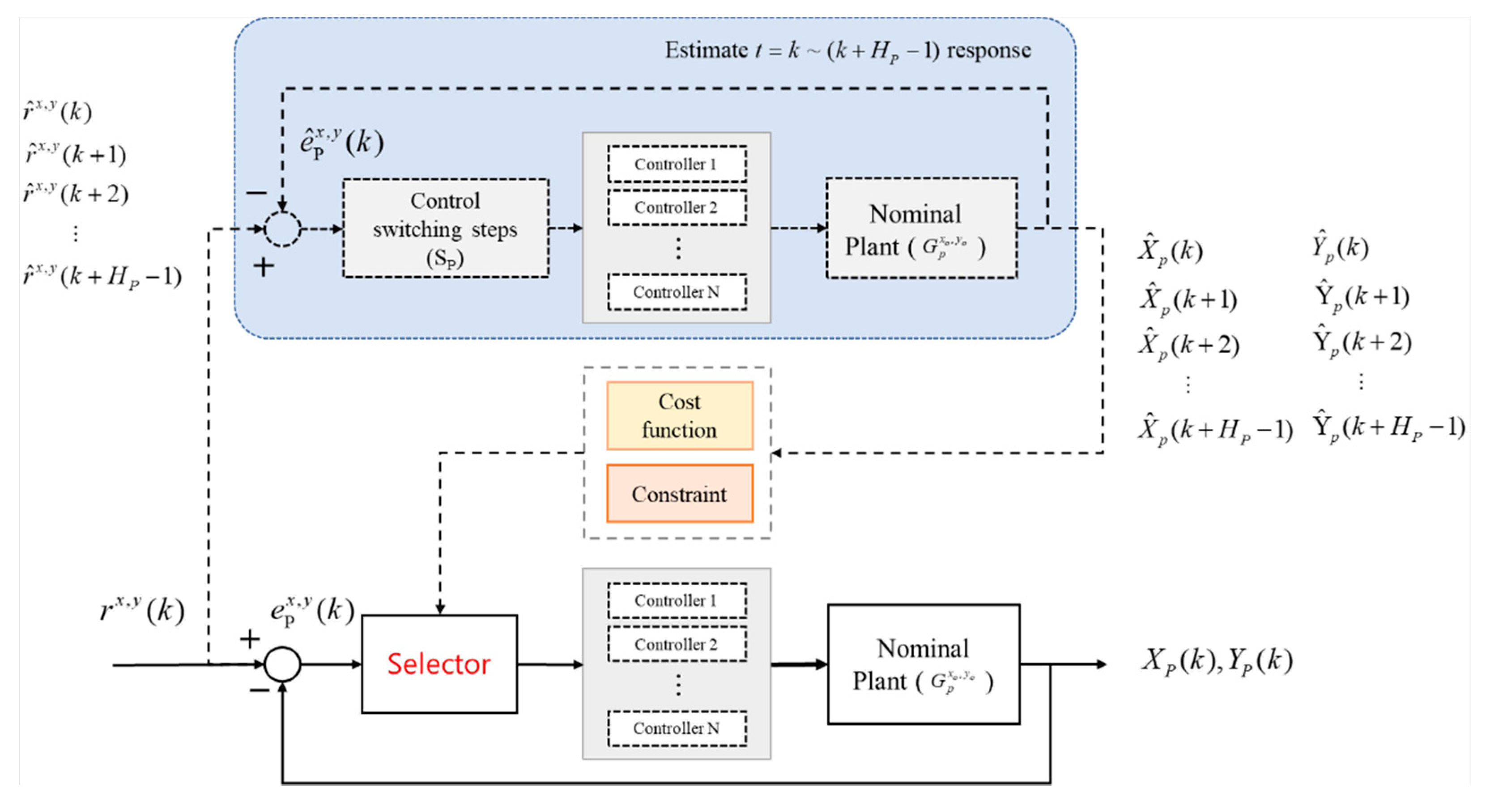
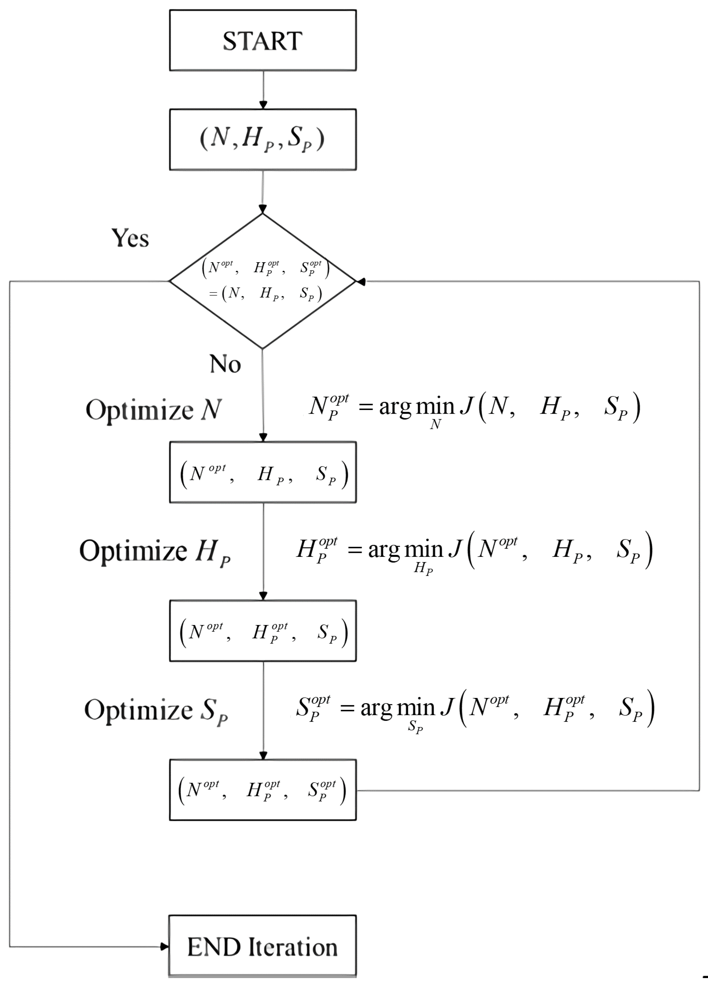
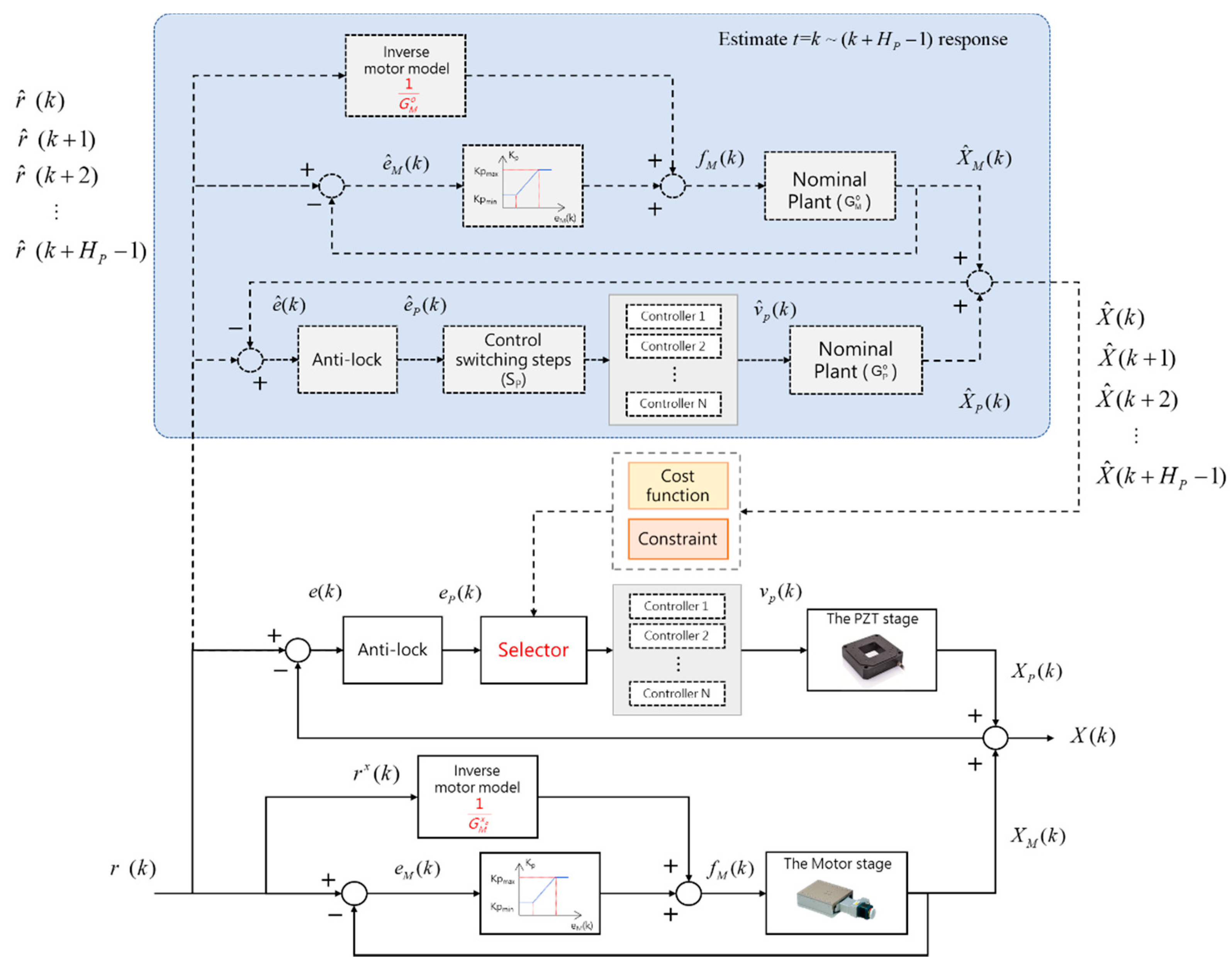
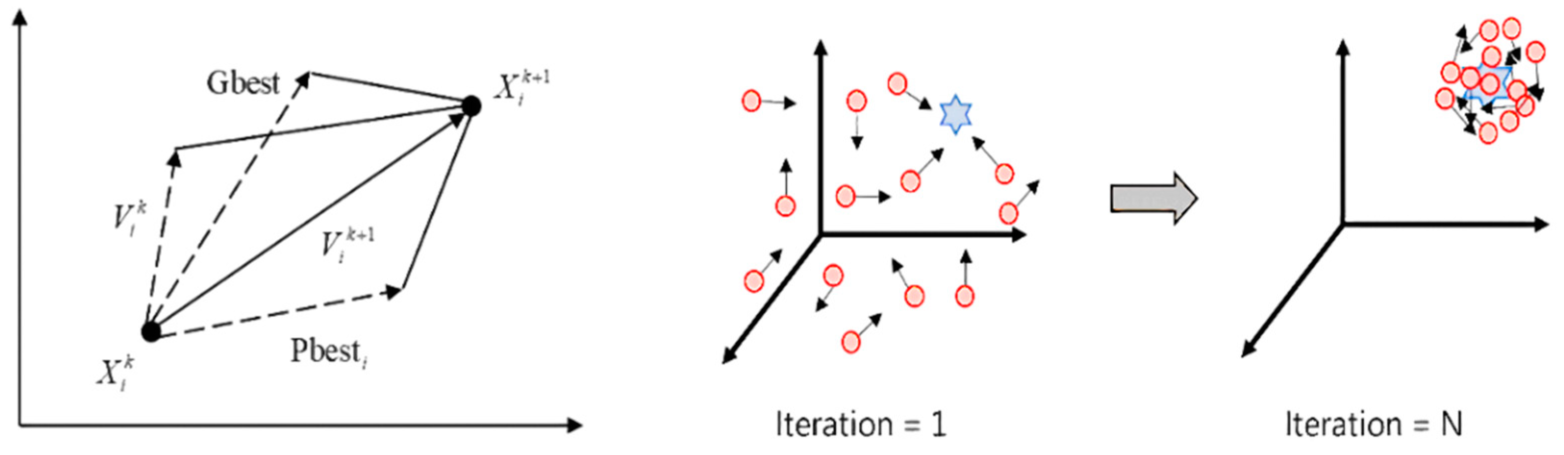
2. Multiple Switching Control with Iterative Parameter Optimization
- Set the default parameters ;
- Apply to derive an optimized N, labelled as , which can improve system performance without exceeding hardware computing limits;
- Apply to derive an optimized , labelled as , which can improve system performance without exceeding hardware computing limits;
- Apply to derive an optimized , labelled as , which can improve system performance without exceeding hardware computing limits;
- If , then the iteration is terminated, and the optimal parameters can be implemented by the multiple control structure. Otherwise, set and return to step 1.
3. Iterative Parameter Optimization for the Long-Stroke Precision Stage Employing Multiple Switching Control
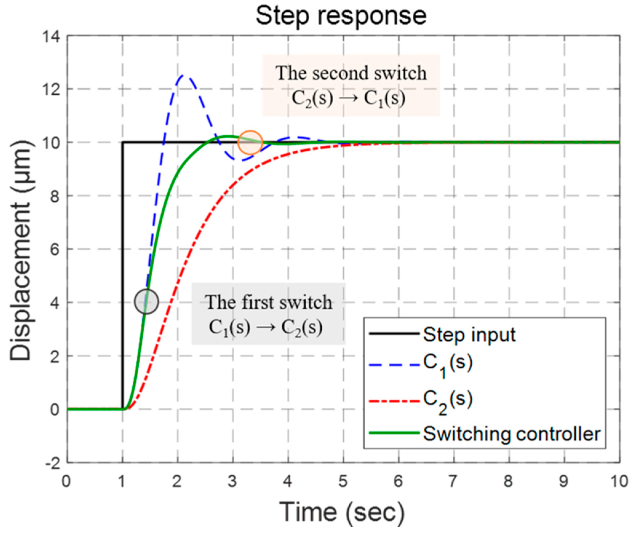
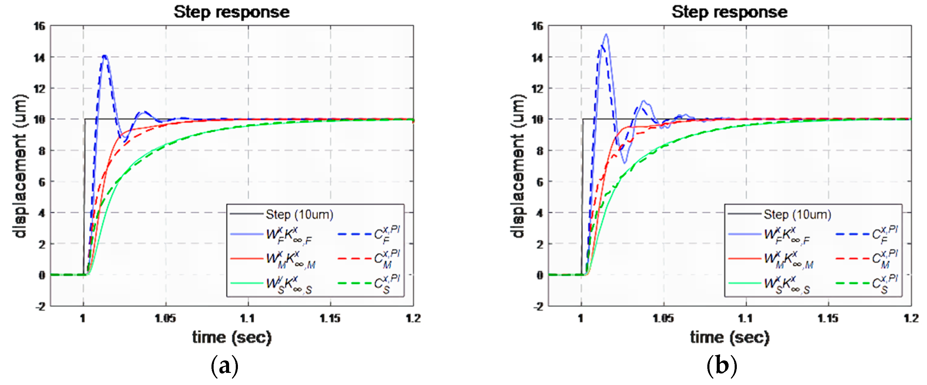
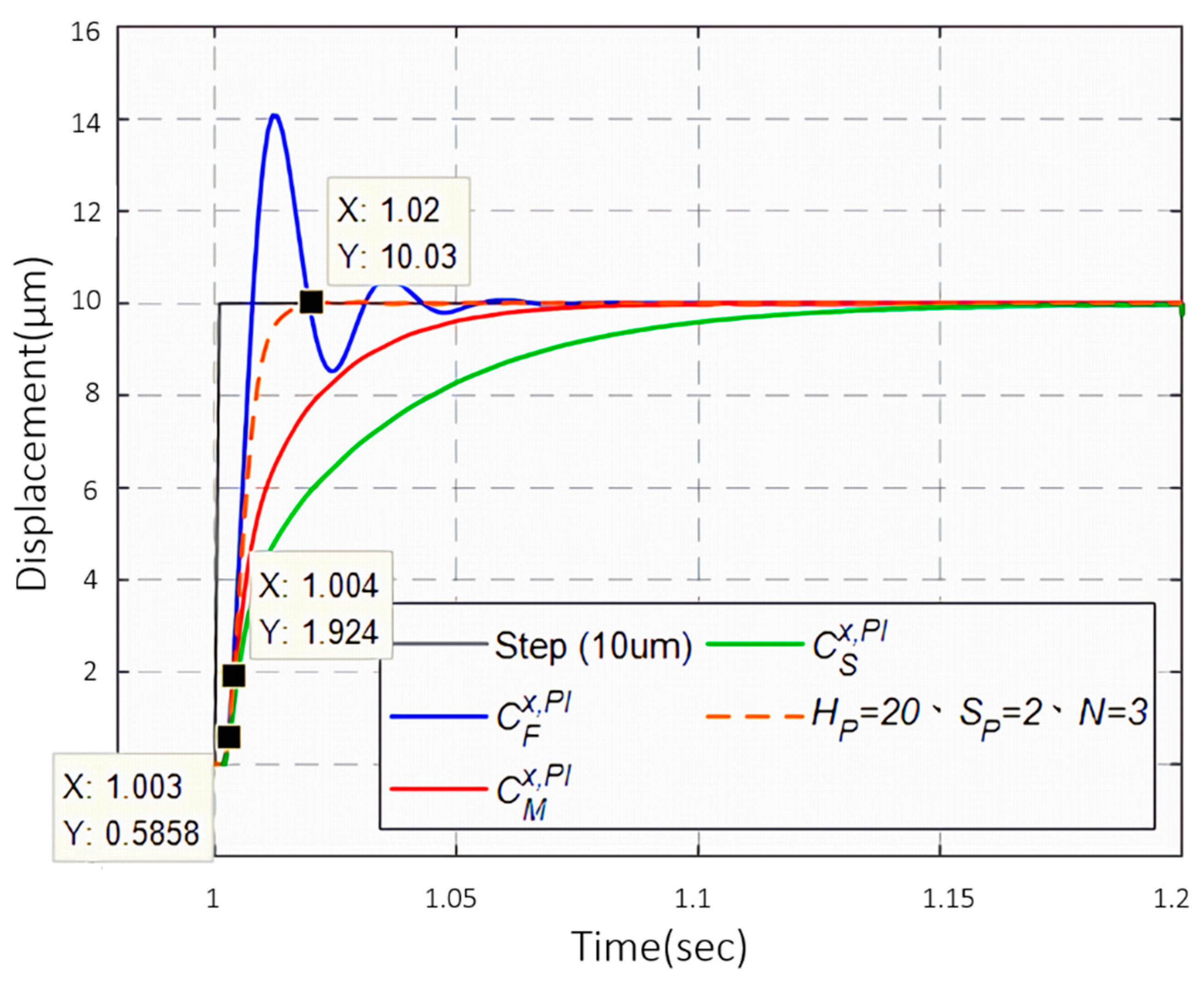
3.1. Multiple Switching Control for the PZT Stage
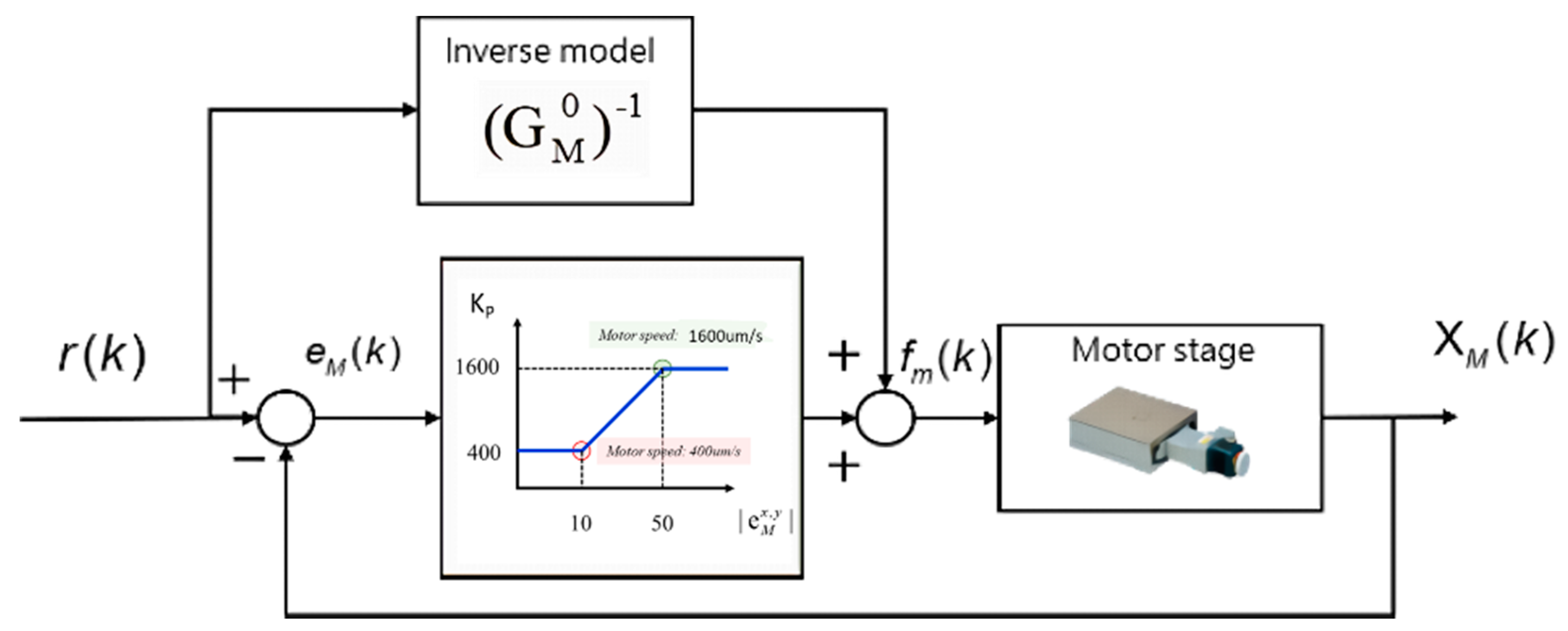
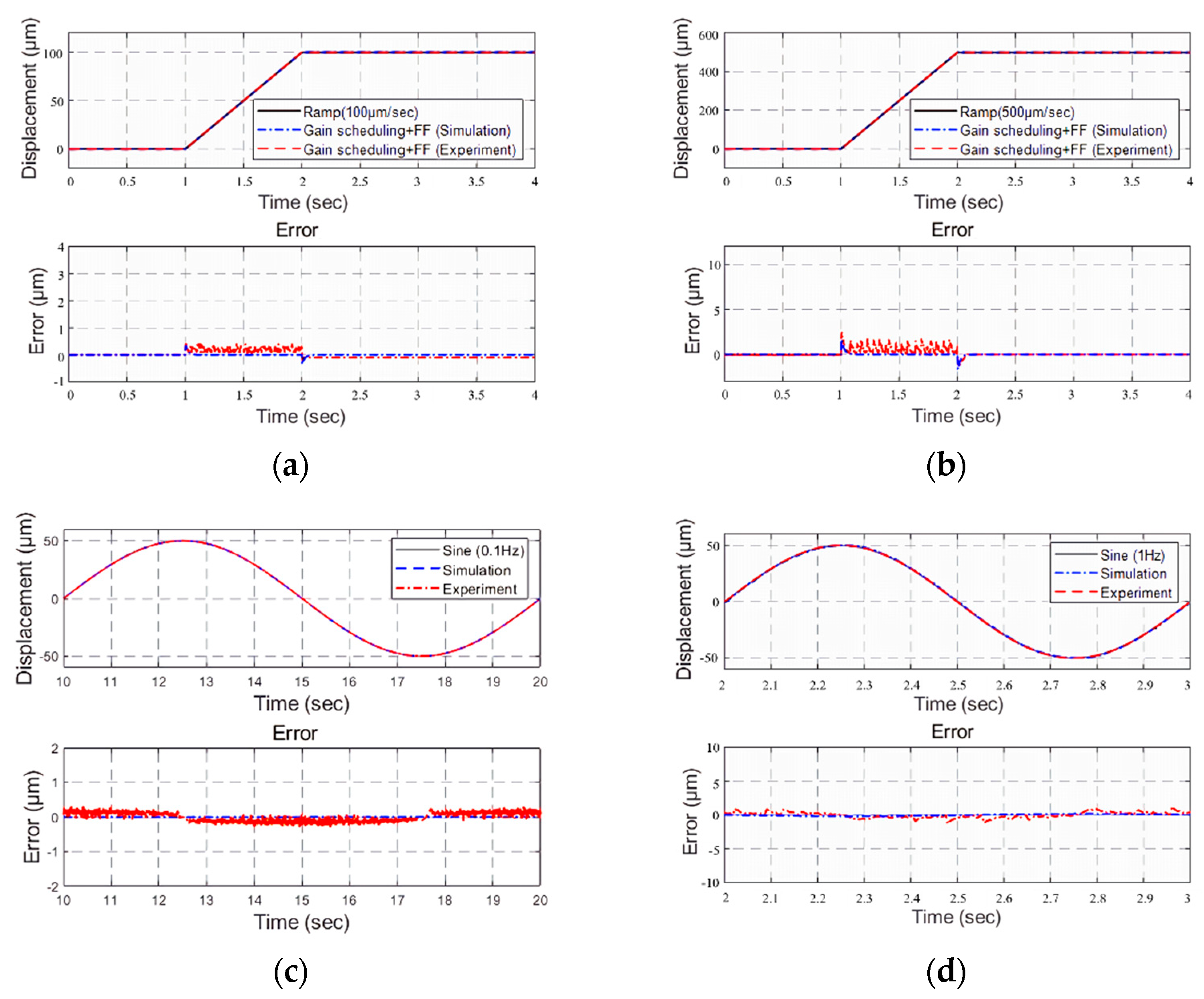
3.2. Switching Control for the Motor Stage
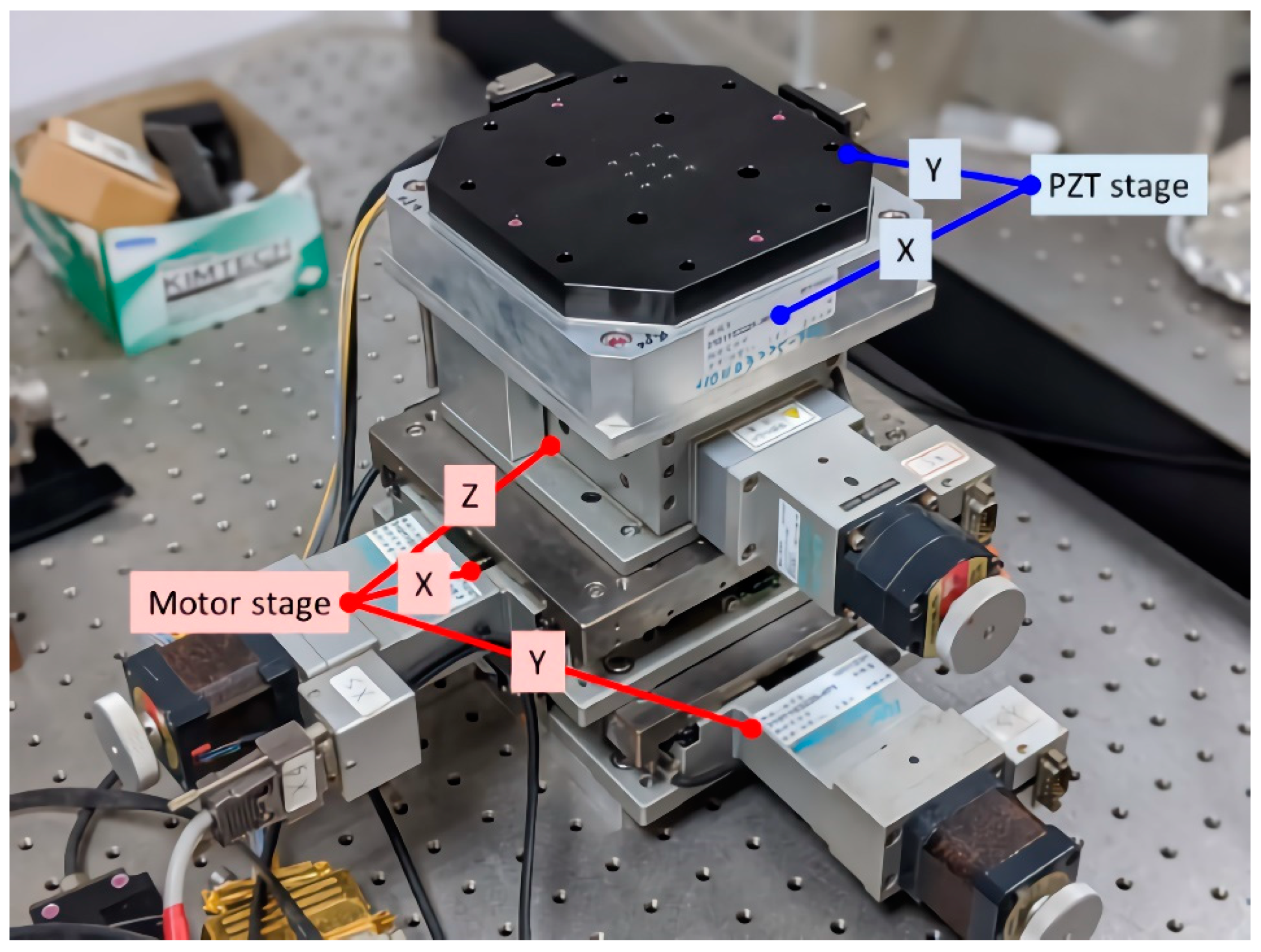
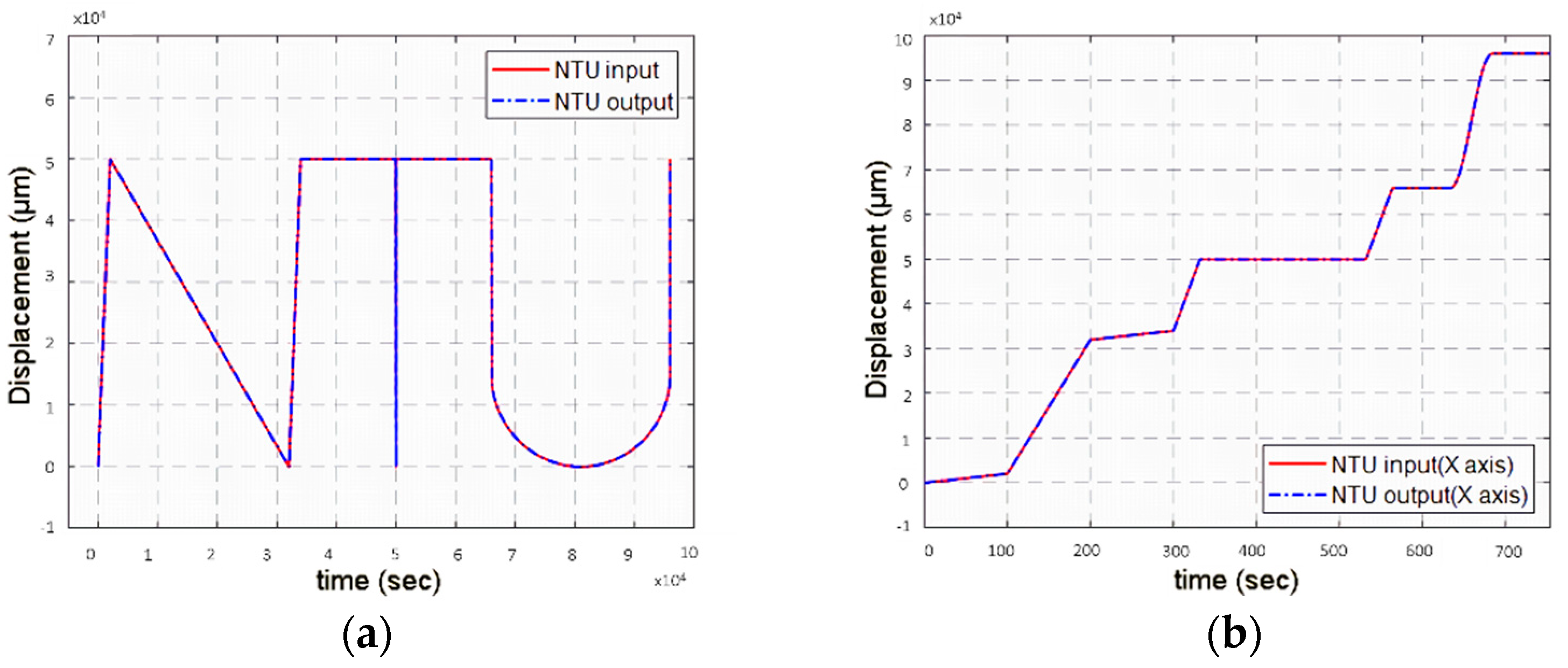
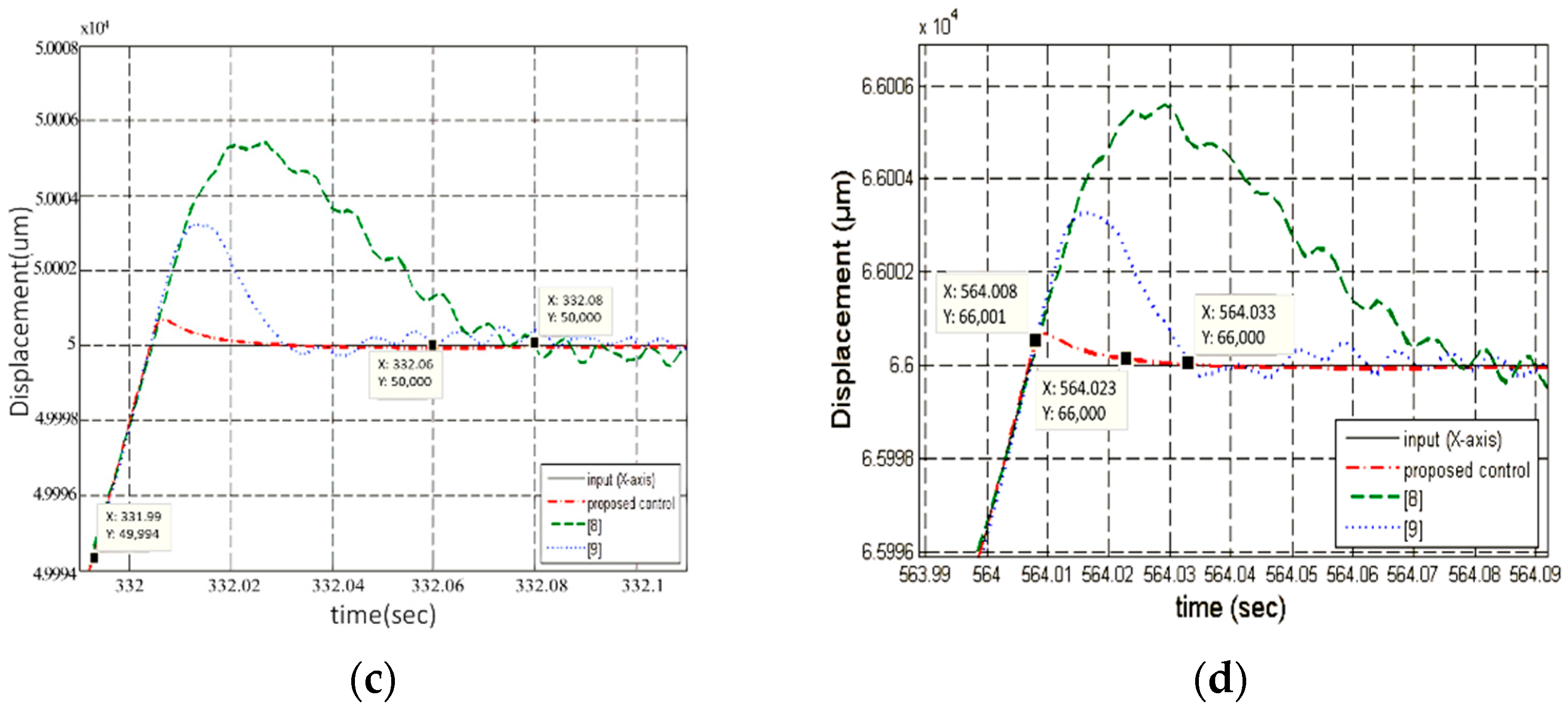
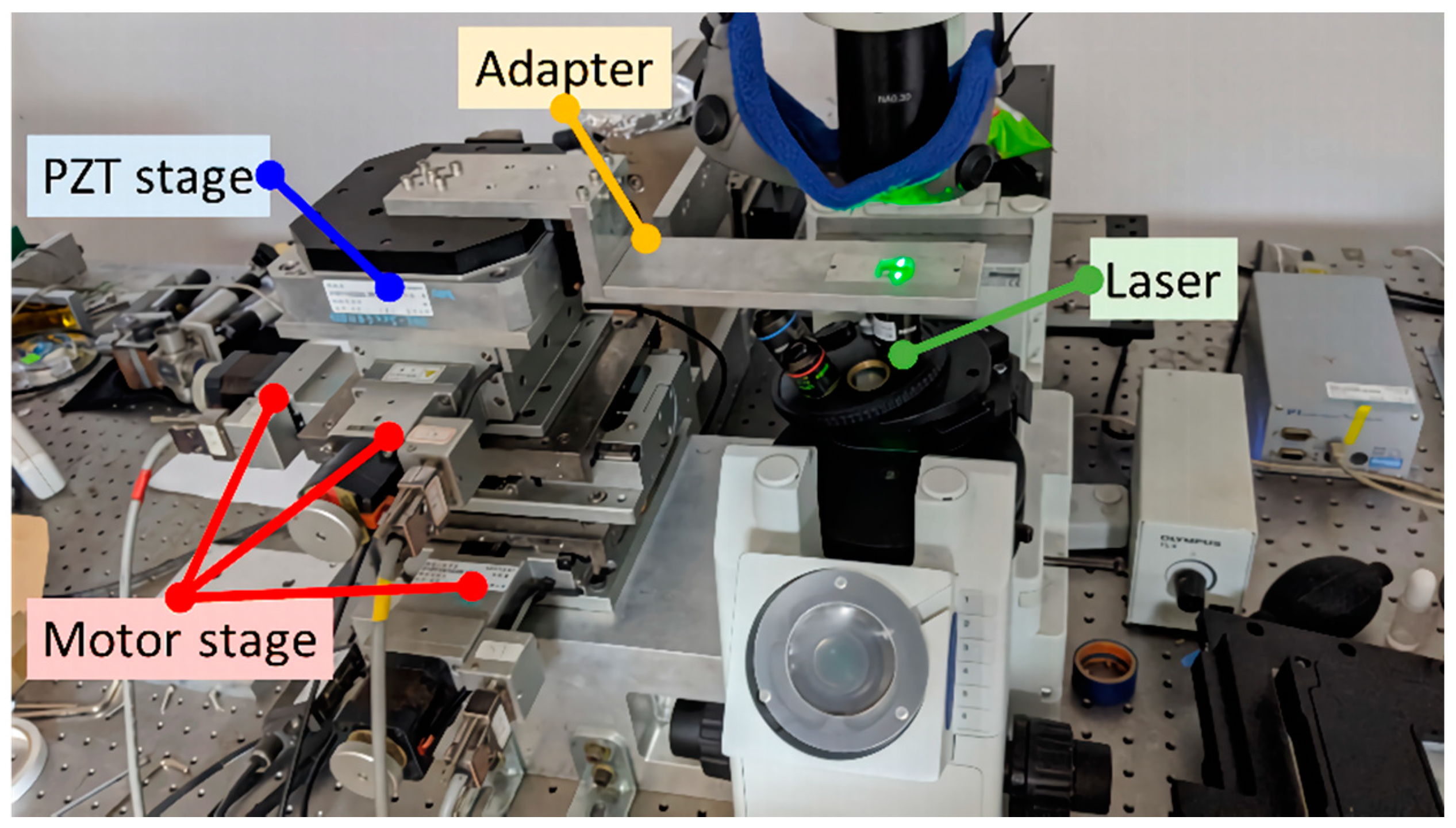
3.3. The Combined Stage
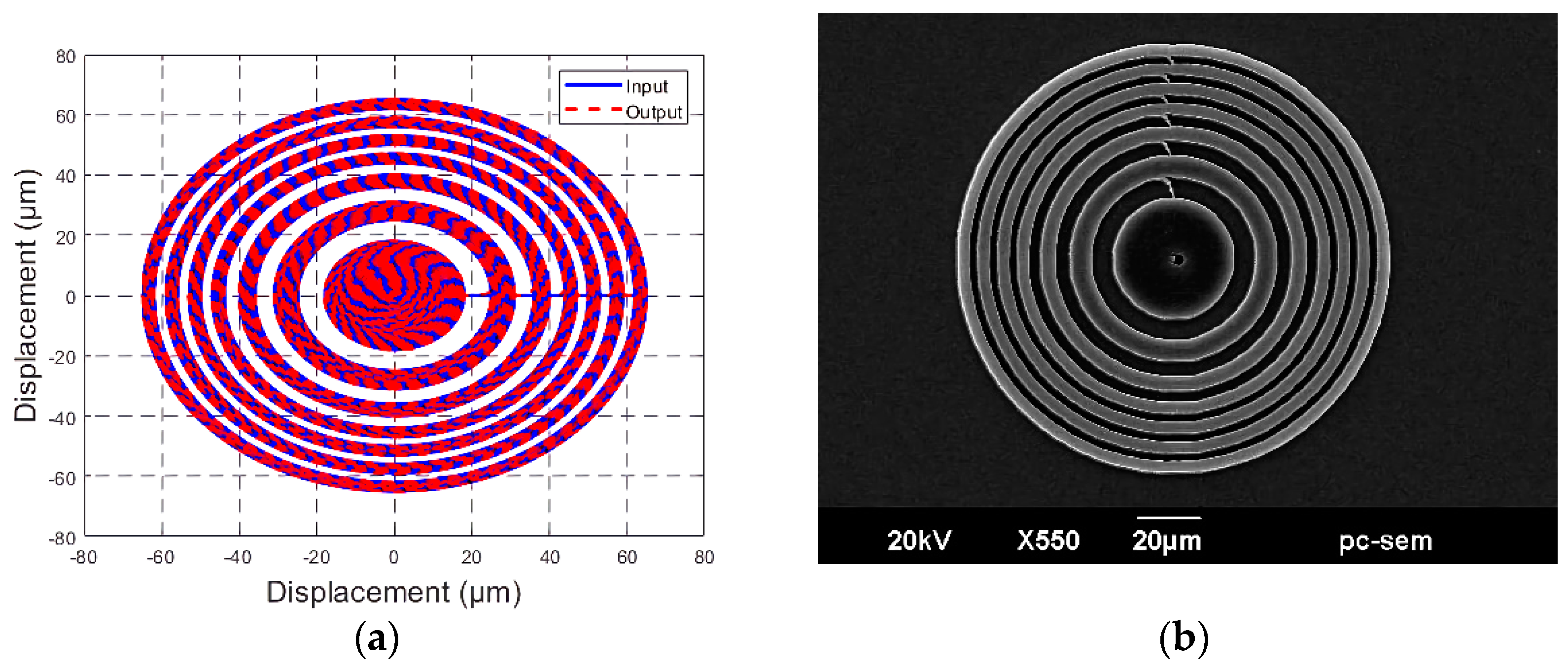
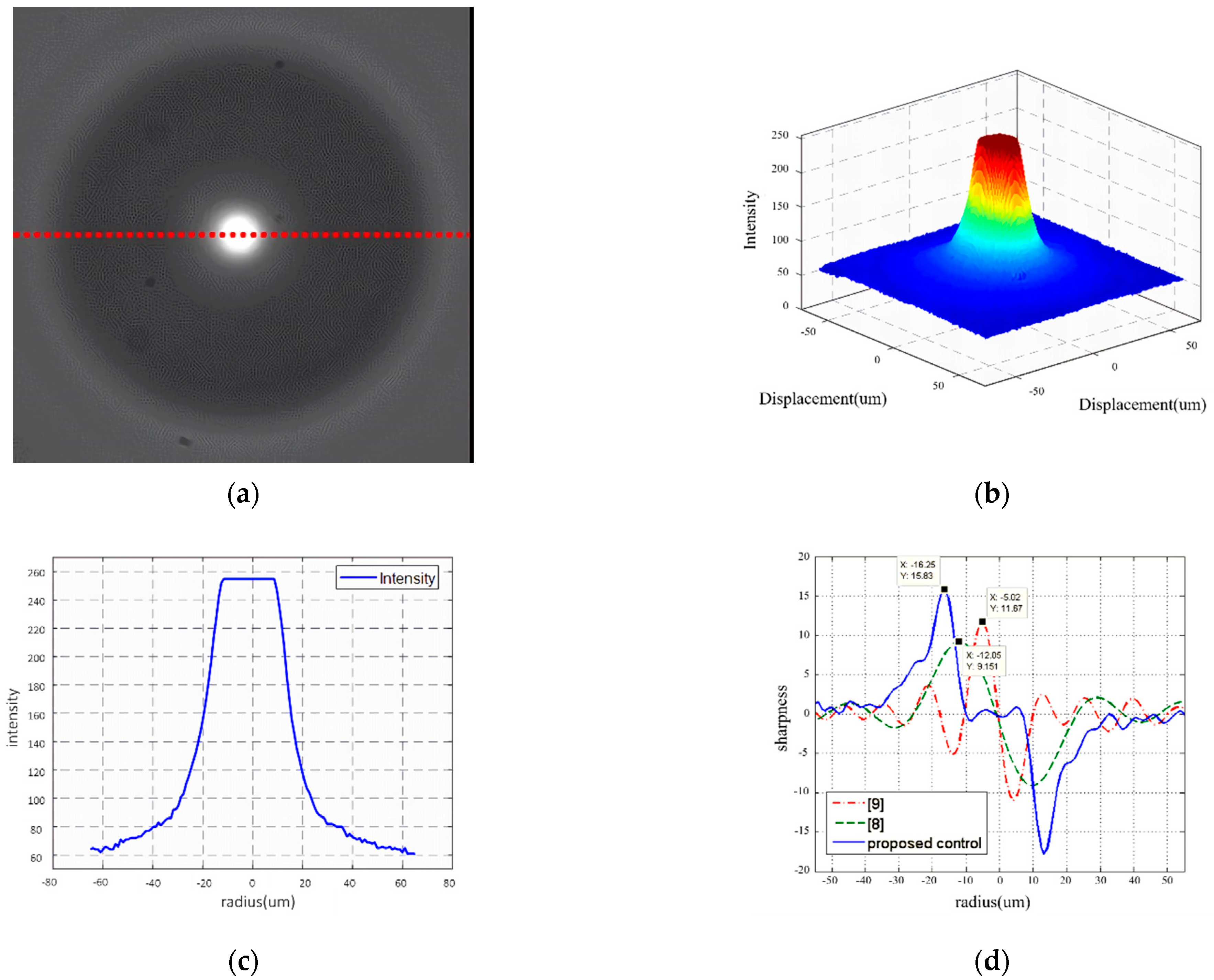
3.4. Microfabrication by Two-Photon Polymerization
4. Conclusions
Author Contributions
Funding
Institutional Review Board Statement.
Informed Consent Statement
Acknowledgments
Conflicts of Interest
Appendix A. Robust Control Design for the PZT Stage
- Increasing the loop gains at low frequencies for disturbance rejection;
- Decreasing the loop gains at high frequencies for noise attenuation;
- Smoothing the magnitude slopes near the crossover frequency for stability consideration.
Appendix B. Robust PI Control Design by the PSO Algorithms

- Stability margin: ;
- Root-mean-square error: ;
- Settling time: = the settling time to a step input;
- Overshoot: = percentage overshoot of a step response;
- Rising time: = rising time to a step input.

| 0.419 | 4.476 × 10⁻⁵ | 2.100 × 10⁻² | 3.000 × 10⁻³ | 5.100 × 10⁻⁵ | ||
| 0.520 | 4.300 × 10⁻³ | 2.000 × 10⁻³ | 5.371 × 10⁻⁵ | 1.200 × 10⁻² | ||
| 0.601 | 8.000 × 10⁻³ | 6.573 × 10⁻⁴ | 0 | 4.000 × 10⁻² |
Appendix C. Iterative Parameter Optimization for the PZT Stage

| Initial Setting Parameters | Optimal Parameters | Costs | |
|---|---|---|---|
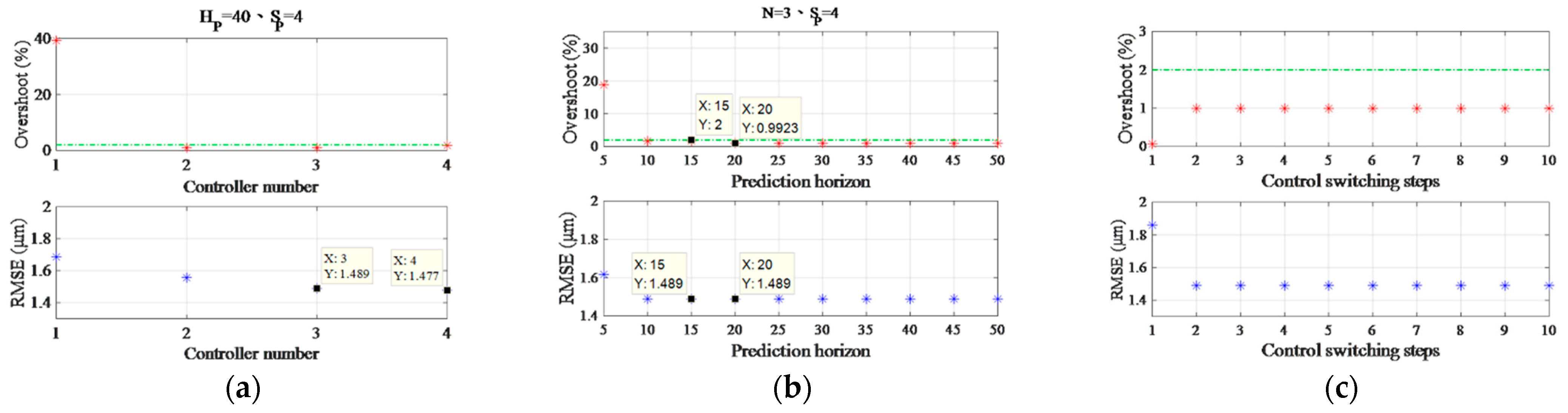
| Fitst iteration | N = 2, J = 1.557 μm N = 3, J = 1.489 μm N = 4, J = 1.477 μm | ||
| Hp =5, J = 1.617 μm Hp = 20, J = 1.489 μm Hp = 40, J = 1.489 μm | |||
| Sp = 1, J = 1.860 μm Sp = 2, J = 1.489 μm Sp = 3, J = 1.489 μm | |||
| Second iteration | N = 2, J = 1.557 μm N = 3, J = 1.489 μm N = 4, J = 1.477 μm | ||
| Hp =5, J = 1.617 μm Hp =20, J = 1.489 μm Hp =40, J = 1.489 μm | |||
| Sp = 1, J = 1.860 μm Sp = 2, J = 1.489 μm Sp = 3, J = 1.489 μm |
References
- Solihin, M.I.; Wahyudi; Legowo, A. Fuzzy-tuned PID anti-swing control of automatic gantry crane. J. Vib. Control 2010, 16, 127–145. [Google Scholar] [CrossRef]
- Bashash, S.; Saeidpourazar, R.; Jalili, N. Tracking control of time-varying discontinuous trajectories with application to probe-based imaging and nanopositioning. In Proceedings of the 2009 American Control Conference, St. Louis, MO, USA, 10–12 June 2009. [Google Scholar]
- Qin, Y.; Sun, L.; Hua, Q.; Liu, P. A fuzzy adaptive PID controller design for fuel cell power plant. Sustainability 2018, 10, 2438. [Google Scholar] [CrossRef] [Green Version]
- Xu, S.; Wang, X.; Yang, J.; Wang, L. A fuzzy rule-based PID controller for dynamic positioning of vessels in variable environmental disturbances. J. Mar. Sci. Technol. 2019, 25, 1–11. [Google Scholar] [CrossRef]
- Armaghan, S.; Moridi, A.; Sedigh, A.K. Design of a switching PID controller for a magnetically actuated mass spring damper. In Proceedings of the World Congress on Engineering, London, UK, 6–8 June 2011; Volume III. [Google Scholar]
- Asl, R.M.; Mahdoudi, A.; Pourabdollah, E.; Klančar, G. Combined PID and LQR controller using optimized fuzzy rules. Soft Comput. 2019, 23, 5143–5155. [Google Scholar]
- Rana, M.; Pota, H.R.; Petersen, I.R. MPC in high-speed atomic force microscopy. In Proceedings of the 2016 Australian Control Conference (AuCC), Newcastle, NSW, Australia, 3–4 November 2016. [Google Scholar]
- Wang, K.-A.; Peng, Y.-K.; Wang, F.-C. The Development and Control of a Long-Stroke Precision Stage. Smart Sci. 2017, 5, 85–93. [Google Scholar] [CrossRef]
- Wang, F.-C.; Peng, Y.-K.; Lu, J.-F.; Chung, T.-T.; Yen, J.-Y. Micro-lens fabrication by a long-stroke precision stage with switching control based on model response prediction. Microsyst. Technol. 2019, 3, 1–14. [Google Scholar] [CrossRef]
- Wang, F.-C.; Lu, J.-F.; Su, W.-J.; Yen, J.-Y. Precision positioning control of a long-stroke stage employing multiple switching control. Microsyst. Technol. 2020, 1, 1–14. [Google Scholar] [CrossRef]
- Nichols, R.A.; Reichert, R.T.; Rugh, W.J. Gain scheduling for H-infinity controllers: A flight control example. IEEE Trans. Control. Syst. Technol. 1993, 1, 69–79. [Google Scholar] [CrossRef] [Green Version]
- Yamaguchi, T.; Shishida, K.; Tohyama, S.; Hirai, H. Mode switching control design with initial value compensation and its application to head positioning control on magnetic disk drives. IEEE Trans. Ind. Electron. 1996, 43, 65–73. [Google Scholar] [CrossRef]
- Hossain, A.; Rahman, M. Comparative Analysis among Single-Stage, Dual-Stage, and Triple-Stage Actuator Systems Applied to a Hard Disk Drive Servo System. Actuators 2019, 8, 65. [Google Scholar] [CrossRef] [Green Version]
- Zhu, W.; Rui, X.-T. Hysteresis modeling and displacement control of piezoelectric actuators with the frequency-dependent behavior using a generalized Bouc–Wen model. Precis. Eng. 2016, 43, 299–307. [Google Scholar] [CrossRef]
- Saleem, A.; Al-Ratrout, S.; Mesbah, M. A fitness function for parameters identification of Bouc-Wen hysteresis model for piezoelectric actuators. In Proceedings of the 5th International Conference on Electrical and Electronic Engineering (ICEEE), Istanbul, Turkey, 3–5 May 2018. [Google Scholar]
- Gan, J.; Zhang, X. Nonlinear hysteresis modeling of piezoelectric actuators using a generalized Bouc–Wen model. Micromachines 2019, 10, 183. [Google Scholar] [CrossRef] [Green Version]
- Fang, J.; Wang, J.; Li, C.; Zhong, W.; Long, Z. A compound control based on the piezo-actuated stage with bouc–wen model. Micromachines 2019, 10, 861. [Google Scholar] [CrossRef] [Green Version]
- Zhang, F.; Liu, J.; Tian, J. Analysis of the Vibration Suppression of Double-Beam System via Nonlinear Switching Piezoelectric Network. Machines 2021, 9, 115. [Google Scholar] [CrossRef]
- Physik Instrumente P-517 • P-527 Multi-Axis Piezo Scanner. Available online: https://www.physikinstrumente.com/en/products/nanopositioning-piezo-flexure-stages/multi-axis-piezo-flexure-stages/p-517-p-527-multi-axis-piezo-scanner-201500/ (accessed on 4 July 2021).
- Piezomechanik Amplifier SVR/150/3. Available online: https://www.piezomechanik.com/products/ (accessed on 4 July 2021).
- Chuo Precision Industrial Stepper Motor ALS-510-H1P. Available online: https://www.chuo.co.jp/contents/hp0543/list.php?CNo=543&ProCon=7065 (accessed on 4 July 2021).
- Chuo Precision Industrial Stepper Motor ALV-104-HP. Available online: https://www.chuo.co.jp/contents/hp0058/list.php?CNo=58&ProCon=94 (accessed on 4 July 2021).
- National Instruments DAQ Card PCI-6221 and PCI-6229. Available online: https://www.ni.com/zh-tw.html (accessed on 4 July 2021).
- Glover, K.; McFarlane, D. Robust stabilization of normalized coprime 457 factor plant descriptions with H/sub infinity/-bounded uncertainty. IEEE 458 Trans. Autom. Control 1989, 34, 821–830. [Google Scholar] [CrossRef]
- Georgiou, T.T.; Smith, M.C. Optimal robustness in the gap metric. In Proceedings of the 28th IEEE Conference on Decision and Control, Tampa, FL, USA, 13–15 December 1989. [Google Scholar]
- McFarlane, D.; Glover, K. A loop-shaping design procedure using H/sub infinity/synthesis. IEEE Trans. Autom. Control 1992, 37, 759–769. [Google Scholar] [CrossRef]
- Kennedy, J.; Eberhart, R. Particle swarm optimization. In Proceedings of the ICNN’95-International Conference on Neural Networks, Perth, WA, Australia, 27 November–1 December 1995. [Google Scholar]
- Meyrán, G.J. Augustin-Jean Fresnel. Rev. Mex. Oftalmol. 2008, 2, 82. [Google Scholar]
- Zhang, Y.; Fang, Y.; Zhou, X.; Dong, X. Image-based hysteresis modeling and compensation for an AFM piezo-scanner. Asian J. Control 2009, 11, 166–174. [Google Scholar] [CrossRef]
- Lu, H.; Fang, Y.; Ren, X.; Zhang, X. Improved direct inverse tracking control of a piezoelectric tube scanner for high-speed AFM imaging. Mechatronics 2015, 31, 189–195. [Google Scholar] [CrossRef]
- Kuo, F.-C.; Hsu, C.; Hsieh, M.-R.; Yen, J.-Y.; Chen, L.-C.; Chung, T.-T.; Wang, F.-C. Study on the transient response to the point-to-point motion controls on a dual-axes air-bearing planar stage. Int. J. Adv. Manuf. Technol. 2020, 111, 2759–2772. [Google Scholar] [CrossRef]
- Liu, L.-C.; Yang, P.-H.; Liao, S.-C.; Li, B.-P.; Wang, F.-C.; Lin, P.-C. Development of a dual-stage and visual-servo filming robot. Proc. Inst. Mech. Eng. Part I J. Syst. Control Eng. 2021, 235, 0959651821991363. [Google Scholar]


| P-517.RCD PZT Stage [19] | |
|---|---|
| Active axis | x, y |
| Maximum stroke | −50 to 50 μm |
| Mass | 1.4 kg |
| Resolution | 1 nm |
| SVR/150/3 amplifier [20] | |
| Output voltage range | −30 to 150 V |
| Max gain | 30 (tunable) |
| ALS-510-H2 P stepper [21] | |
| Active axis | x, y |
| Maximum stroke | 100 mm |
| Resolution | 0.1 μm |
| Maximum loading | 40 kgf |
| Maximum command | 80,000 pulse/sec |
| ALV-104-HP stepper [22] | |
| Active axis | z |
| Maximum stroke | 40 mm |
| Resolution | 0.1 μm |
| Maximum loading | 10 kgf |
| Maximum command | 40,000 pulse/sec |
| Robust Controller | Robust PI Controller | ||||||
|---|---|---|---|---|---|---|---|
| Sim. | Rise time (sec) | 0.0043 | 0.0171 | 0.0622 | 0.0051 | 0.0327 | 0.0692 |
| Settling time (sec) | 1.0415 | 1.0612 | 1.1331 | 1.0563 | 1.0654 | 1.1283 | |
| Overshoot (%) | 41.1600 | 0 | 0 | 39.2792 | 0.0101 | 0 | |
| RMSE (μm) | 1.6834 | 2.0511 | 2.6434 | 1.6863 | 1.8733 | 2.5951 | |
| Exp. | Rise time (sec) | 0.0043 | 0.0158 | 0.0622 | 0.0038 | 0.0287 | 0.0654 |
| Settling time (sec) | 1.0647 | 1.0579 | 1.1269 | 1.0495 | 1.0574 | 1.1183 | |
| Overshoot (%) | 54.8200 | 0.1100 | 0 | 47.4300 | 0.2100 | 0.0500 | |
| RMSE (μm) | 1.8872 | 2.1419 | 2.7021 | 1.6934 | 1.9034 | 2.4406 | |
| Inputs | Ramp | Sinusoidal | |||
|---|---|---|---|---|---|
| Sizes | 100 μm/s | 500 μm/s | 0.1 Hz | 1 Hz | |
| Sim. | Phase lag (°) | - | - | 0 | 0 |
| Maximum error (μm) | 0.3324 | 1.6622 | 0.0017 | 0.171 | |
| RMSE (μm) | 0.0401 | 0.2007 | 0.0013 | 0.2939 | |
| Exp. | Phase lag (º) | - | - | 0 | 0 |
| Maximum error (μm) | 0.4000 | 2.5000 | 0.3000 | 1.1267 | |
| RMSE(μm) | 0.2238 | 0.7851 | 0.1355 | 0.4161 | |
Publisher’s Note: MDPI stays neutral with regard to jurisdictional claims in published maps and institutional affiliations. |
© 2021 by the authors. Licensee MDPI, Basel, Switzerland. This article is an open access article distributed under the terms and conditions of the Creative Commons Attribution (CC BY) license (https://creativecommons.org/licenses/by/4.0/).
Share and Cite
Wang, F.-C.; Lu, J.-F.; Chung, T.-T.; Yen, J.-Y. Iterative Parameter Optimization for Multiple Switching Control Applied to a Precision Stage for Microfabrication. Machines 2021, 9, 153. https://doi.org/10.3390/machines9080153
Wang F-C, Lu J-F, Chung T-T, Yen J-Y. Iterative Parameter Optimization for Multiple Switching Control Applied to a Precision Stage for Microfabrication. Machines. 2021; 9(8):153. https://doi.org/10.3390/machines9080153
Chicago/Turabian StyleWang, Fu-Cheng, Jun-Fu Lu, Tien-Tung Chung, and Jia-Yush Yen. 2021. "Iterative Parameter Optimization for Multiple Switching Control Applied to a Precision Stage for Microfabrication" Machines 9, no. 8: 153. https://doi.org/10.3390/machines9080153