Design and Comparison of Reinforcement-Learning-Based Time-Varying PID Controllers with Gain-Scheduled Actions

Abstract

This paper presents innovative reinforcement learning methods for automatically tuning the parameters of a proportional integral derivative controller. Conventionally, the high dimension of the Q-table is a primary drawback when implementing a reinforcement learning algorithm. To overcome the obstacle, the idea underlying the n-armed bandit problem is used in this paper. Moreover, gain-scheduled actions are presented to tune the algorithms to improve the overall system behavior; therefore, the proposed controllers fulfill the multiple performance requirements. An experiment was conducted for the piezo-actuated stage to illustrate the effectiveness of the proposed control designs relative to competing algorithms.

1. Introduction

Recent advances in technology have ushered in the fourth industrial revolution (4IR), a concept introduced by Klaus Schwab [1] that includes three-dimensional (3D) printing, virtual reality, and artificial intelligence (AI), with AI being the most active [1]. As presented in [2], the branches of AI include expert systems, machine learning (ML), robotics, computer vision, planning, and natural language processing (NLP). ML is when an algorithm learns from data. ML comes in supervised learning, unsupervised learning, and reinforcement learning variants [3].

In supervised learning, the training set contains both the inputs and desired outputs. The training set is used to teach the model to generate the desired output, and the goal of supervised learning is to learn a mapping between the input and the output spaces [3]. Supervised learning was often used in image recognition, and self-supervised semi-supervised learning (S4L) was proposed to solve the image classification problem [4]. In unsupervised learning, the training set contains unlabeled inputs that do not have any assigned desired output. 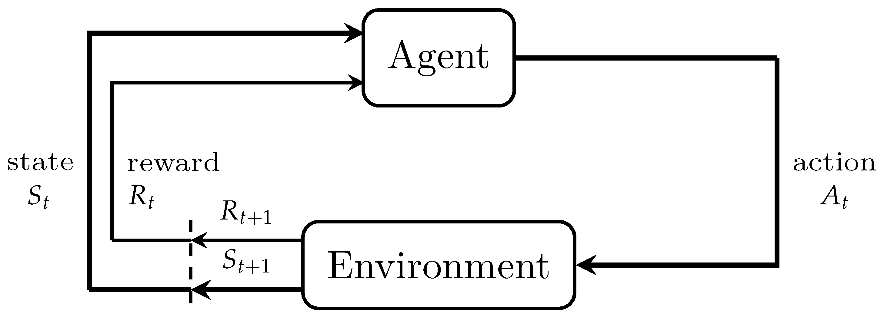The goal of unsupervised learning is typically to discover the properties of the data generating process, and its applications include clustering documents with similar topics [3] or identifying the phases and phase transitions of systems [5]. Reinforcement learning is similar to supervised and unsupervised learning and has advantages of both. Some form of supervision exists, but reinforcement learning does not require a desired output to be specified for each input in the data; the reinforcement learning algorithm receives feedback from the environment only after selecting an output for a given input or observation [3]. In other words, the building system model is unnecessary for reinforcement learning algorithms [6].

In reinforcement learning, the most challenging problem is finding the best trade-off between exploration and exploitation; this trade-off dominates the performance of the agent. By combining Monte Carlo methods and dynamic programming (DP) ideas, temporal difference (TD) learning is a brilliant solution to the problems of reinforcement learning. Two TD control methods, Q-learning and Sarsa, were proposed on the basis of the TD learning method [7]. Q-Learning [8] is a form of model-free reinforcement learning. It can also be viewed as a method of asynchronous DP. It provides agents with the capability of learning to act optimally in Markovian domains by experiencing the consequences of actions without requiring maps of the domains to be built [9,10]. The Sarsa algorithm was first explored in 1994 by Rummery and Niranjan [11] and was termed modified Q-learning. In 1996, the name Sarsa was introduced by Sutton [7].

Conventionally, Sarsa and Q-learning have been applied to robotics problems [11]. Recently, a fuzzy Sarsa learning (known as FSL) algorithm was proposed to control a biped walking robot [12] and a PID-SARSA-RAL algorithm was proposed in the ClowdFlows platform to improve parallel data processing [13]. Q-learning is often applied in combination with a proportional integral derivative (PID) controller. Specifically, an adaptive PID controller was proposed in [14], a self-tuning PID controller for a soccer robot was proposed in [15], and a Q-Learning approach was used to tune an adaptive PID controller in [16]. Moreover, the Q-learning algorithm was applied to the tracking problem for discrete-time systems with an $H_{\infty }$ approach [17] and linear quadratic tracking control [18,19]. Recently, some relevant applications of model-free reinforcement learning for tracking problems can be found in [20,21]. In these results [12,13,14,15,16,17,18], the PID controller has attracted substantial attention as an application of reinforcement learning algorithms [13,14,15,16]. However, the literature [13,15,16,17,18] has provided optimal but static gains in control, and a complete search of the Q-table is required in [14]. Moreover, most of the results [12,13,14,16,17,18,19] were validated in a simulated environment.

For the time-varying PID control design, conventional approaches in the literature can be found as gain-scheduled PID control [22,23], fuzzy PID control [24,25,26,27], or fuzzy gain-scheduling PID control [28,29], in which the fuzzy logic were utilized to determine the controller parameters instead of directly producing the control signal. Nowadays, the application of fuzzy PID control can be found in the automatic voltage regulator (AVR) system [30], hydraulic transplanting robot control system [31], and the combination with fast terminal sliding mode control [32].

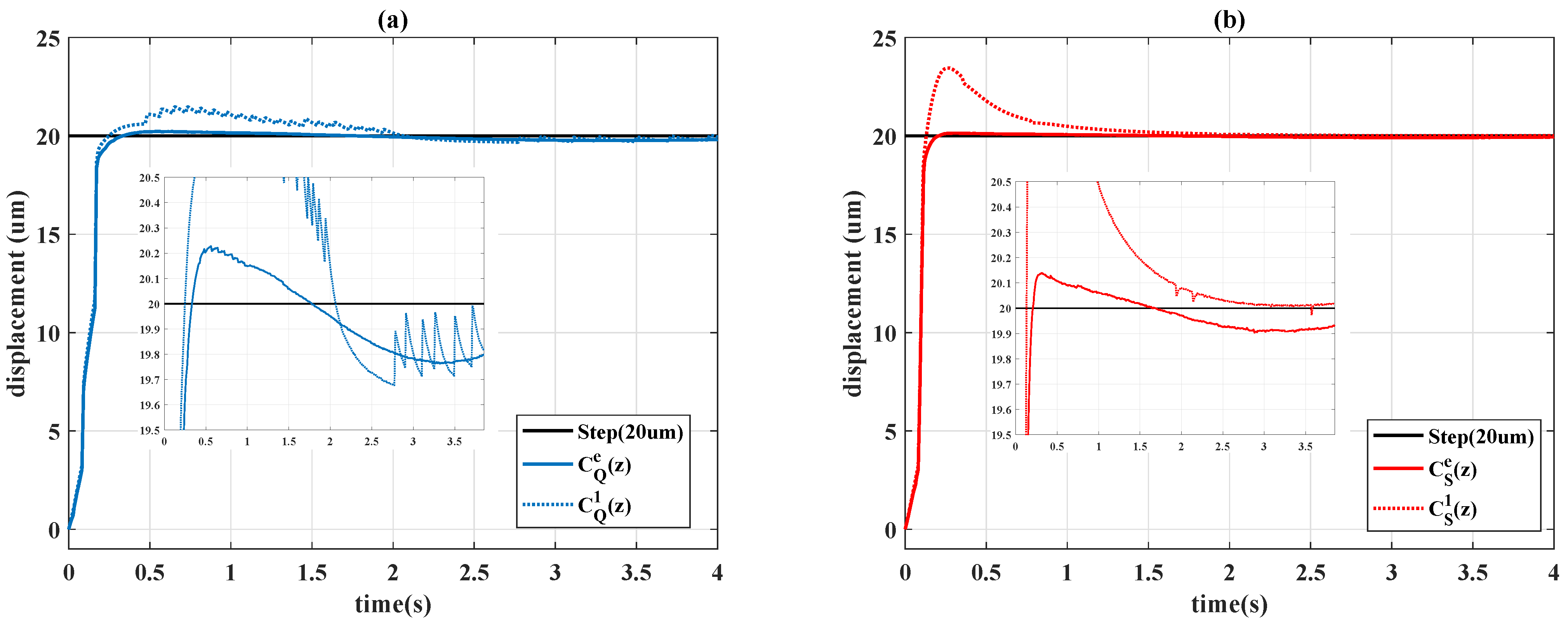
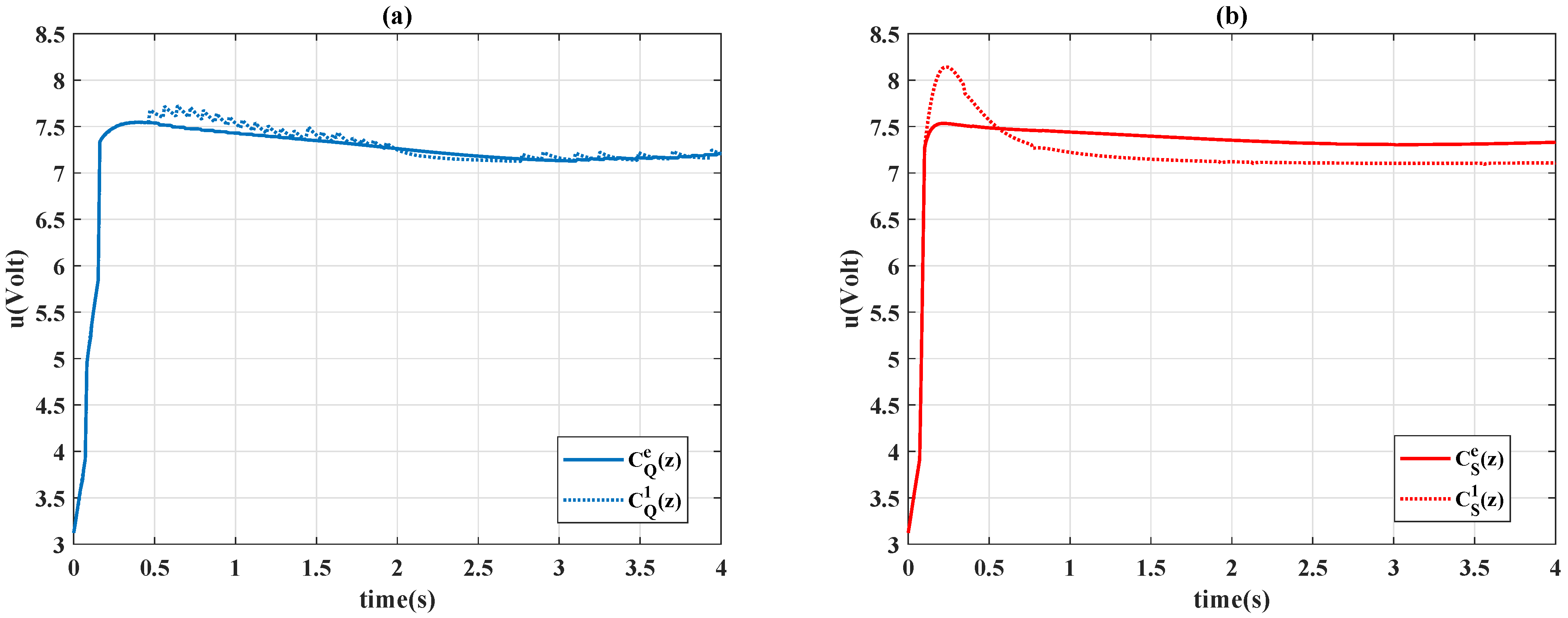
In this paper, a time-varying PID controller following the structure in [28], which features the use of a model-free reinforcement learning algorithm, was proposed to achieve reference tracking in the absence of any knowledge of system dynamics. Based on the concept underlying the n-armed bandit problem [33,34], this study’s method allows for the control coefficients to be assigned online without a complete searching process for the Q-table. The time-varying control gains were capable of achieving the various performance requirements and have the potential to handle nonlinear effects. Both the Q-learning and Sarsa algorithms were applied in the proposed control design, and the performance was compared with experimental results on a piezo-actuated stage.

2. Preliminaries and System Modeling

In this section, the essential concepts of reinforcement learning for controller design are reviewed, and the system modeling of control target (the piezo-actuated stage) is presented.

2.1. The Markov Property

For the finite number of states and reward values, the environment responds at time $t+1$ depending on information from every past event, and the dynamics can be defined only by specifying the complete probability distribution:

$$\begin{array}{c}\hfill Pr\{R_{t+1}=r,S_{t+1}=s^{\prime }|S_0,A_0,R_1,\cdots ,S_{t-1},A_{t-1},R_{t-1},S_t,A_t,R_t\}\end{array}$$

for all reward R, the state after the movement $s^{\prime }$, and possible values of the past events: $S_0,A_0,R_1,\cdots ,S_{t-1},A_{t-1},R_{t-1},S_t,A_t,R_t$. If the state signal has the Markov property, the environment’s response at $t+1$ depends only on the state and action representations at t, in which case the environment’s dynamics can be defined by

$$\begin{array}{c}\hfill p(s^{\prime },r|s,a)=Pr\{R_{t+1}=r,S_{t+1}=s^{\prime }|S_t,A_t\},\end{array}$$

where $p(s^{\prime },r|s,a)$ denotes the probability of transitioning to state $s^{\prime }$ with reward r, from s and a. A reinforcement learning process that satisfies the Markov property is called a Markov decision process (MDP). Moreover, if the state and action spaces are finite, then it is called a finite Markov decision process (finite MDP) [7].

2.2. Reinforcement Learning

Reinforcement learning problems feature an interaction between an agent and environment. The learner—and decision maker—is called the agent, which is what we focused on in our design. The agent interacts with the environment, which is everything external to the agent [7].

As presented in Figure 1, the agent and environment interact at discrete time steps in a sequence, $t=0,1,2,3,\dots$. At each time step t, the agent receives some representation of the environment’s state, $S_t\in S$, where S is the set of possible states. The state is the available signal from the environment that the agent concerns for making decisions. The agent then selects an action $A_t\in A\left(S_t\right)$, where $A\left(S_t\right)$ is the set of actions available in the state $S_t$. One time step later, depending on the action selected by the agent, the agent receives a numerical reward, $R_{t+1}$∈R$\subset \mathbb{R}$, where R is the set of possible rewards, and it then proceeds to a new state $S_{t+1}$. Based on the reward trajectory after time step t and by using a positive discounted factor $\gamma \in \mathbb{R}$, the expected discounted return for time step t is defined as

$$G_t=\sum _{k=0}^{\infty }{\gamma }^k{R}_{t+k+1},$$

where k denotes the kth iteration and $\gamma$ is the discounted factor that satisfies $0\le \gamma \le 1$.

Most reinforcement learning algorithms estimate a value function that evaluates the favorability of the agent being in a given state. The term “favorability” here indicates the magnitude of the expected future rewards. Value functions come in one of two types: the state-value function and the action-value function. The state-value function is the expected discounted return that can be obtained from some state s following some policy $\pi$, and the action-value function is the expected discounted return when state s is the initial state, action a is taken, and policy $\pi$ is followed [7]. Here, we consider the general stochastic policy $\pi \left(a\right|s)$; in this policy, the probability of taking action a under state s satisfies ${\sum }_a\pi \left(a\right|s)=1$. The state-value function $V_{\pi }\left(s\right)$ and the action-value function $Q_{\pi }(s,a)$ for policy $\pi$ can be defined as follows:

$$V_{\pi }\left(s\right)=E_{\pi }\left[G_t\right|S_t=s]=E_{\pi }[\sum _{k=0}^{\infty }{\gamma }^k{R}_{t+k+1}|S_t=s],$$

and

$$Q_{\pi }(s,a)=E_{\pi }\left[G_t\right|S_t=s,A_t=a]=E_{\pi }[\sum _{k=0}^{\infty }{\gamma }^k{R}_{t+k+1}|S_t=s,A_t=a],$$

where $E_{\pi }[·]$ represents the expectation value of the expected discounted return under policy $\pi$ [7].

2.3. Q-Learning

A key breakthrough in reinforcement learning was the development of an off-policy TD control algorithm known as Q-learning [8]. One-step Q-learning is defined by

$$Q_Q(S_t,A_t)\leftarrow Q_Q(S_t,A_t)+\alpha [R_{t+1}+\gamma \underset{a}{max}{Q}_Q(S_{t+1},a)-Q_Q(S_t,A_t)],$$

(1)

where $\alpha <1$ is a positive number known as the learning rate, and the lower script notation for the action-value function denotes the Q-learning algorithm. The algorithm is presented in procedural form in Algorithm 1 [7].

Algorithm 1 Q-learning: Off-policy TD control algorithm.

Initialize $Q(s,a)$, $\forall s\in S$, $a\in A\left(s\right)$, arbitrarily, and $Q(terminal-state,·)=0$ repeat (for each episode):     Initialize S     repeat (for each step of episode):         Choose A from S using a policy derived from $Q(e.g.,ϵ-greedy)$         Take action A, observe $R,S^{\prime }$         $Q(S,A)\leftarrow Q(S,A)+\alpha [R+\gamma {max}_{a}Q(S^{\prime },a)-Q(S,A)]$         $S\leftarrow S^{\prime };$     until S is terminal until episode has terminated

Algorithm 1 is such that (1) the $ϵ$-greedy policy strategy is the selection of the action with the maximum Q value and a probability of $1-ϵ$ in a certain state and (2) an action is randomly selected from all possible actions for the state with probability $ϵ$, which can be expressed as

$$\pi \left(a\right|s)=\{\begin{array}{c}1-ϵ+{\displaystyle \frac{ϵ}{\left|A\right(s\left)\right|}},\mathrm{if} a=arg\underset{a\in A\left(s\right)}{max}Q(s,a)\hfill \\ {\displaystyle \frac{ϵ}{\left|A\right(s\left)\right|}},\mathrm{otherwise},\hfill \end{array}$$

(2)

where $\left|A\right(s\left)\right|$ represents the number of all possible actions in state s [7].

2.4. Sarsa

As an on-policy TD control method that uses TD prediction methods for the control problem, the Sarsa algorithm is defined by the update of the action-value function:

$$Q_S(S_t,A_t)\leftarrow Q_S(S_t,A_t)+\alpha [R_{t+1}+\gamma Q_S(S_{t+1},A_{t+1})-Q_S(S_t,A_t)].$$

(3)

This rule uses every element of the quintuple of events $(S_t,A_t,R_{t+1},S_{t+1},A_{t+1})$ that compose a transition from one state–action pair to the next. The algorithm is named Sarsa, based on the symbols for the elements in the quintuple. The general form of the Sarsa control algorithm is given in Algorithm 2 [7].

Algorithm 2 Sarsa: On-policy TD control algorithm.

Initialize $Q(s,a)$, $\forall s\in S$ and $a\in A\left(s\right)$, arbitrarily, and $Q(terminal-state,·)=0$ repeat (for each episode):     Initialize S     Choose A from S using policy derived from $Q(e.g.,ϵ-greedy)$     repeat (for each step of the episode):         Take action A, observe $R,S^{\prime }$         Choose A from S using a policy derived from $Q(e.g.,ϵ-greedy)$         $Q(S,A)\leftarrow Q(S,A)+\alpha [R+\gamma {max}_{a}Q(S^{\prime },A^{\prime })-Q(S,A)]$         $S\leftarrow S^{\prime };$$A\leftarrow A^{\prime }$     until S is terminal until episode has terminated

2.5. System Modeling of Piezo-Actuated Stage

We formulated the model of the piezoelectric transducer (PZT) with reference to [35]. As presented in Figure 2, the PZT model is divided into two subsystems: mechanical and electrical. In a mechanical subsystem, the behavior follows that of a standard mass-spring-damper system. We shall adopt the following notation. $F_p$ is the output force generated by the piezoelectric actuator, $F_{ext}$ is the external applied force, $K_p$ is the stiffness constant, ${\Lambda }_p$ is the damping constant, and ${\Delta }_p$ is the elongation of the piezoelectric transducer. In the electrical subsystem, the input voltage u contributes a linear transduction voltage $u_p$, and $u_h$ is the voltage consumed by the hysteresis effect $H\left(q\right)$. Here, q is the charge flow of the PZT. In the closed loop of circuit, C is an equivalent internal capacitance, and $T_{em}$ is the transformation ratio for the connected mechanical and electrical subsystems. Based on the derivation in [36], a block diagram of a piezo-actuated stage is presented in Figure 3, where G is the linear, time-invariant transfer function of the mechanical stage body.

On the basis of these preliminaries, the goal of this paper is to propose a reinforcement learning-based PID controller that drives the system output to track a reference signal despite the system being affected by nonlinear hysteresis $H\left(q\right)$. The coefficients in the controller are automatically adjusted by the selected learning algorithm.

Remark 1.

In Section 2.3 and Section 2.4, it is seen that the update of state-value function follows a finite MDP; therefore, it is essential to check if the piezo-actuated stage system model fulfills an MDP. According to the block diagram in Figure 3, the action is the adjustment of control gains and the state is system output performance; therefore, the system model inherently follows an MDP since the system transfer function G is linear and time invariant.

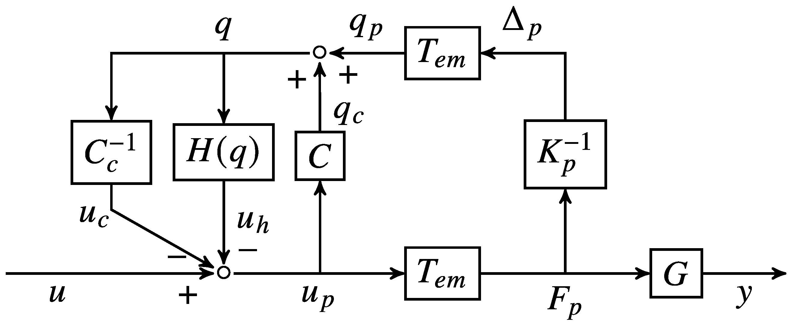
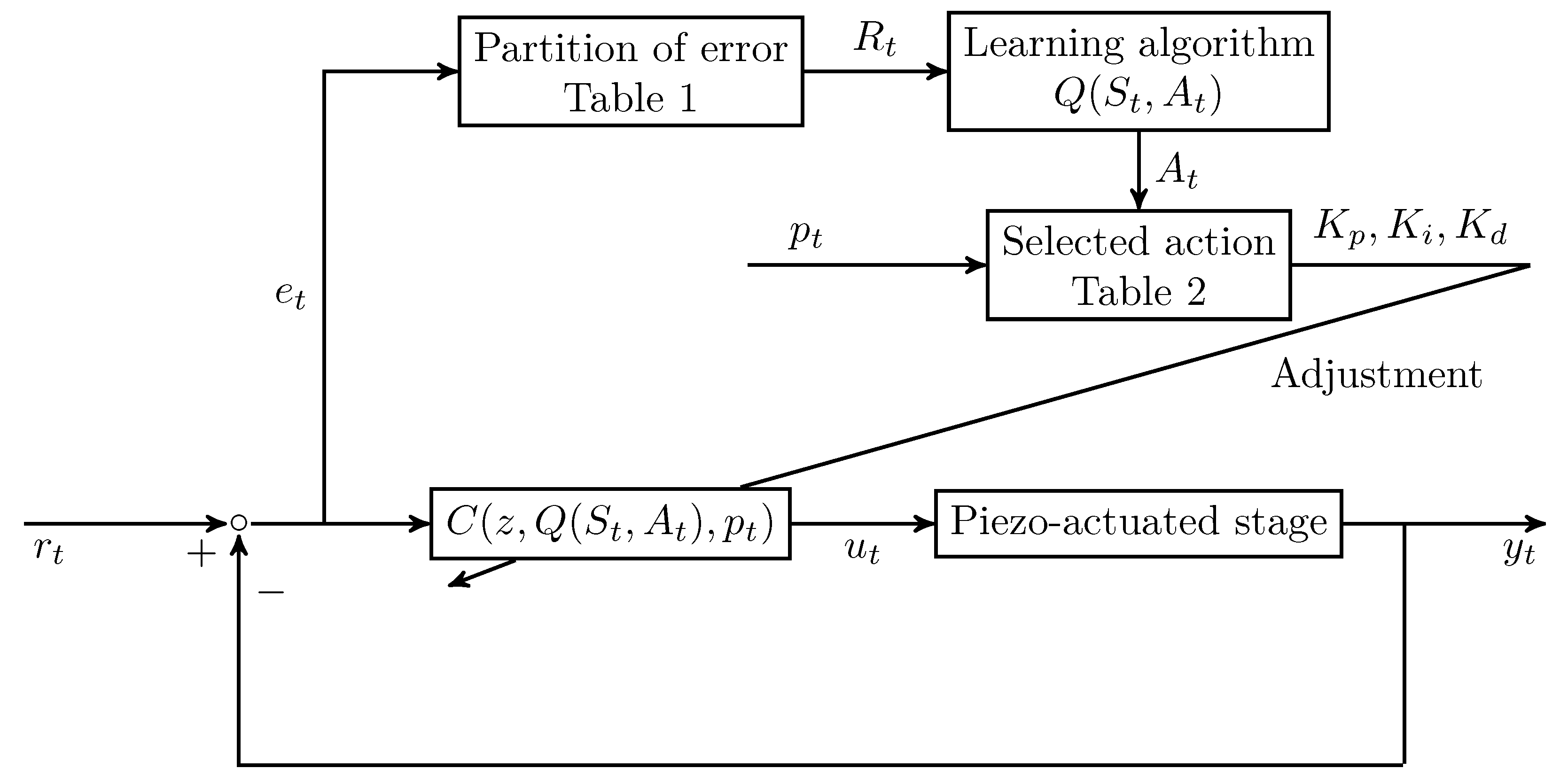
3. Controller Design

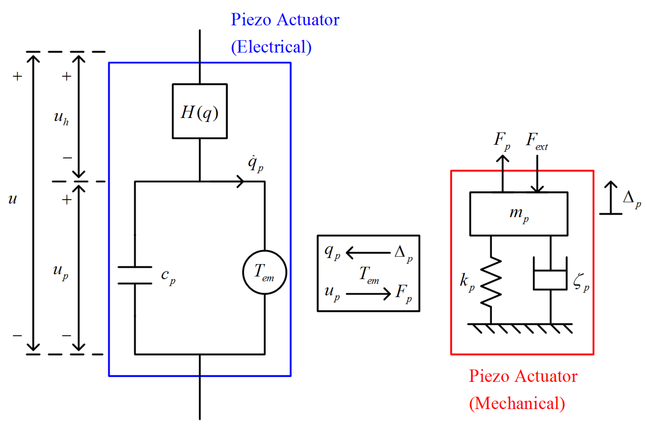
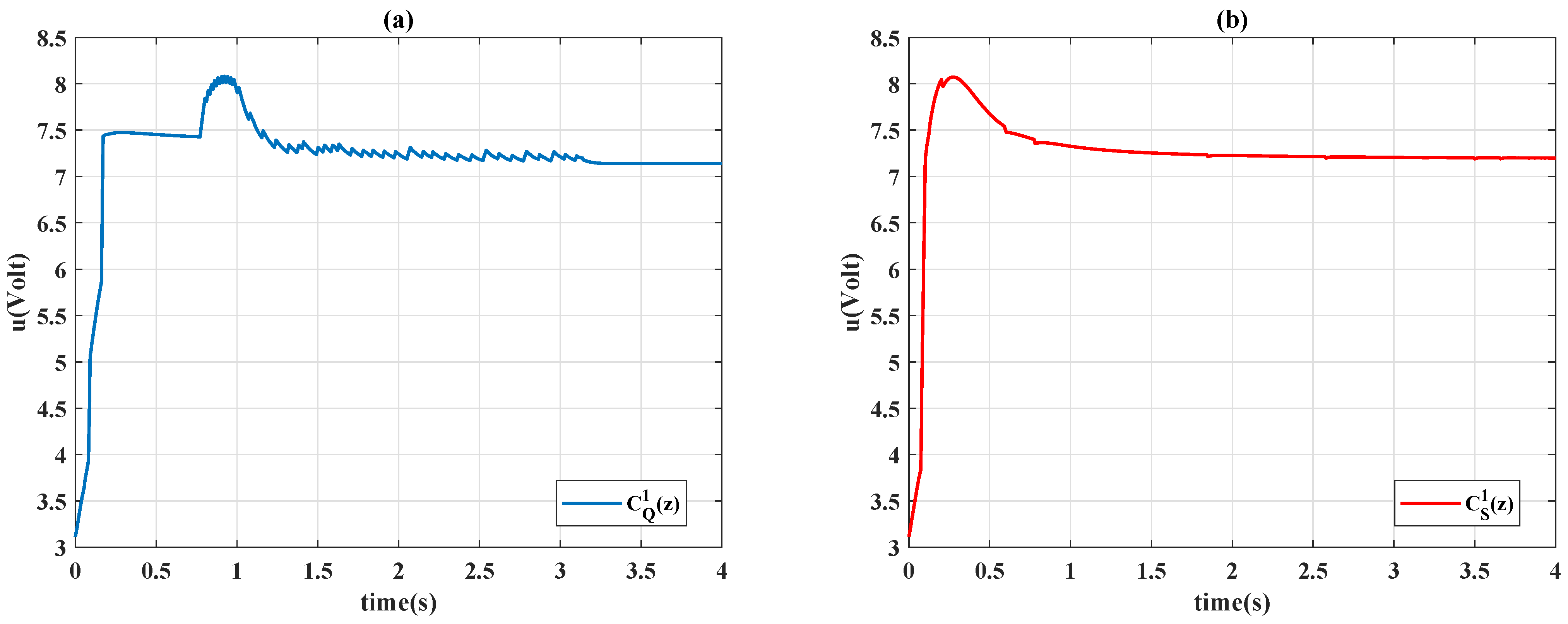
In this section, we describe our fundamental scheme of the time-varying PID controller. According to [37], the control input $u_t$ of the controller in discrete-time is defined as

$$u_t=K_p{e}_t+K_i\sum _{i=0}^k{e}_t\Delta t+K_d{\displaystyle \frac{e_t-e_{t-1}}{\Delta t}}$$

(4)

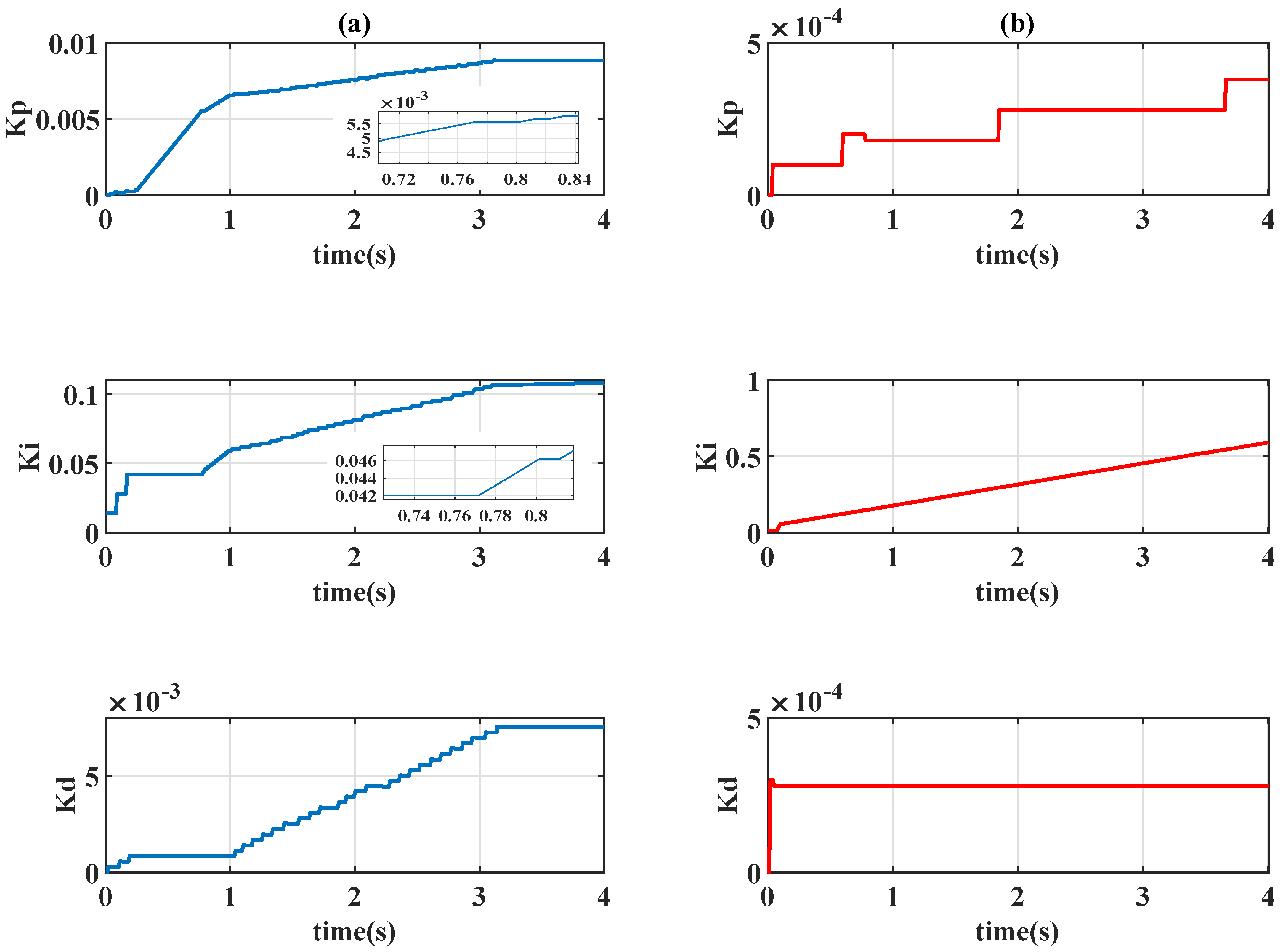
where t is the discrete time index; $\Delta t$ is the time interval of sampling; $K_p$, $K_i$, and $K_d$ are the proportional, integral, and derivative gains, respectively; and the error signal $e_t=r_t-y_t$ is defined in terms of the system output $y_t$ and desired reference $r_t$. Control design typically requires a compromise between various performance requirements; therefore, time-varying PID gains were used to simultaneously achieve multiple requirements. 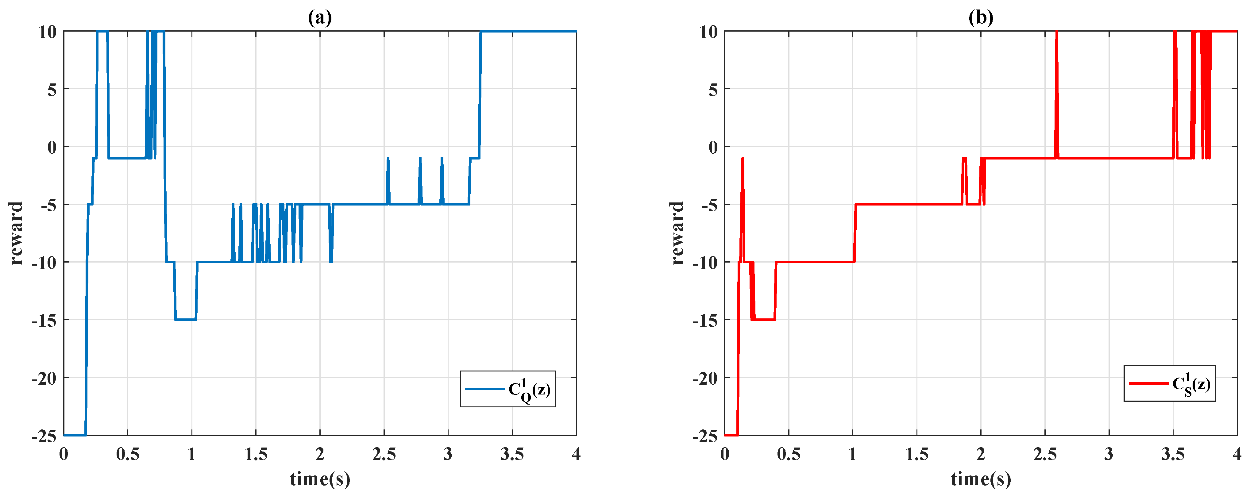In each time step t, a numerical reward $R_t$ is received by the agent according to the partitions in

Table 1. Range of partition error and corresponding reward $R_t$.

Range of Partition	${\mathit{R}}_{\mathit{t}}$
1 $< |e_t|$	−25
0.5 $< |e_t| \le$ 1	−15
0.1 $< |e_t| \le$ 0.5	−10
0.03 $< |e_t| \le$ 0.1	−5
0.01 $< |e_t| \le$ 0.03	−1
others	10

, and the control gains $K_p$, $K_i$, and $K_d$ are adjusted by the chosen actions according to a learning algorithm. This design concept coincides with the original form of the n-armed bandit problem [33,34], and the parameter specification is thus straightforward.

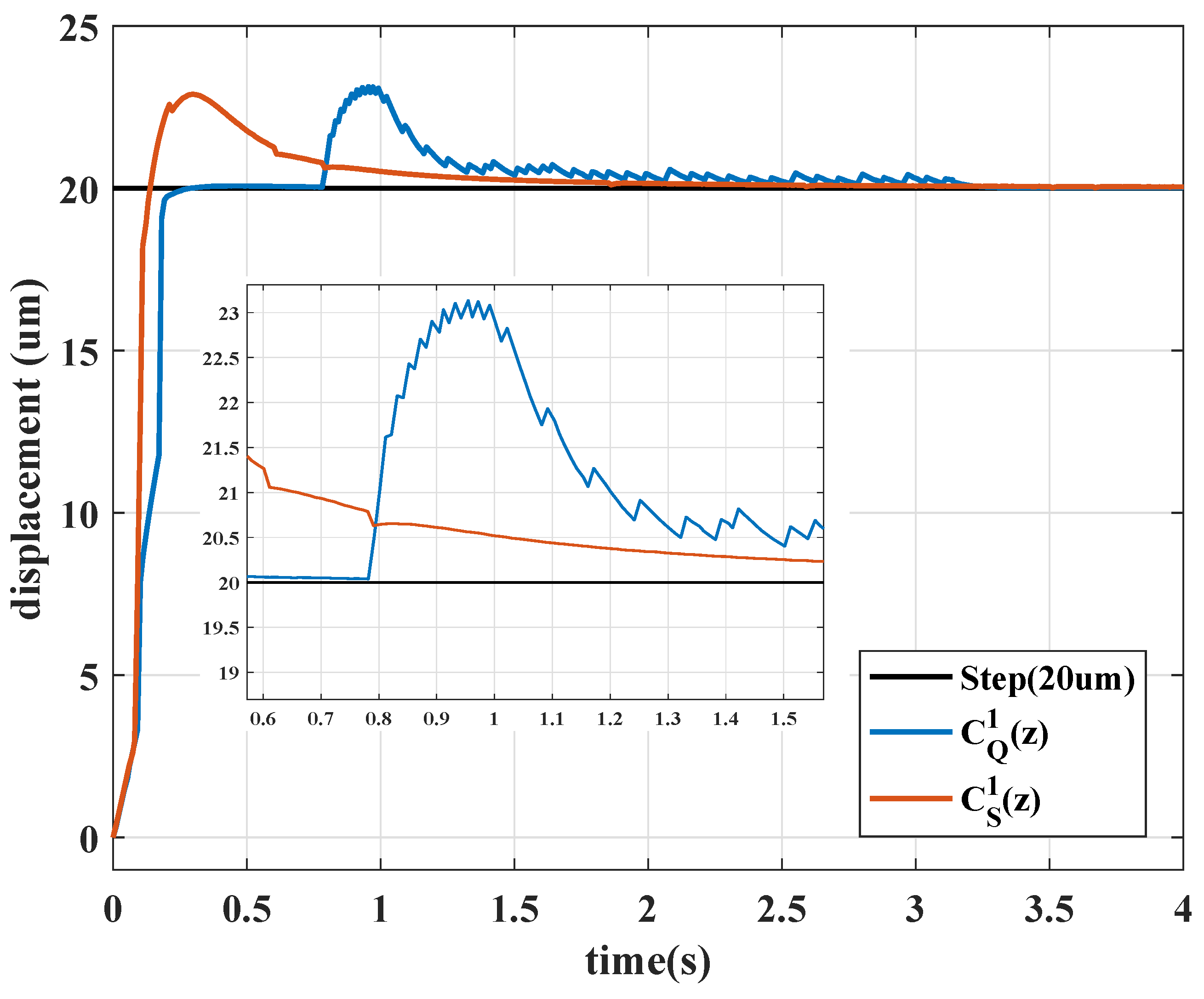
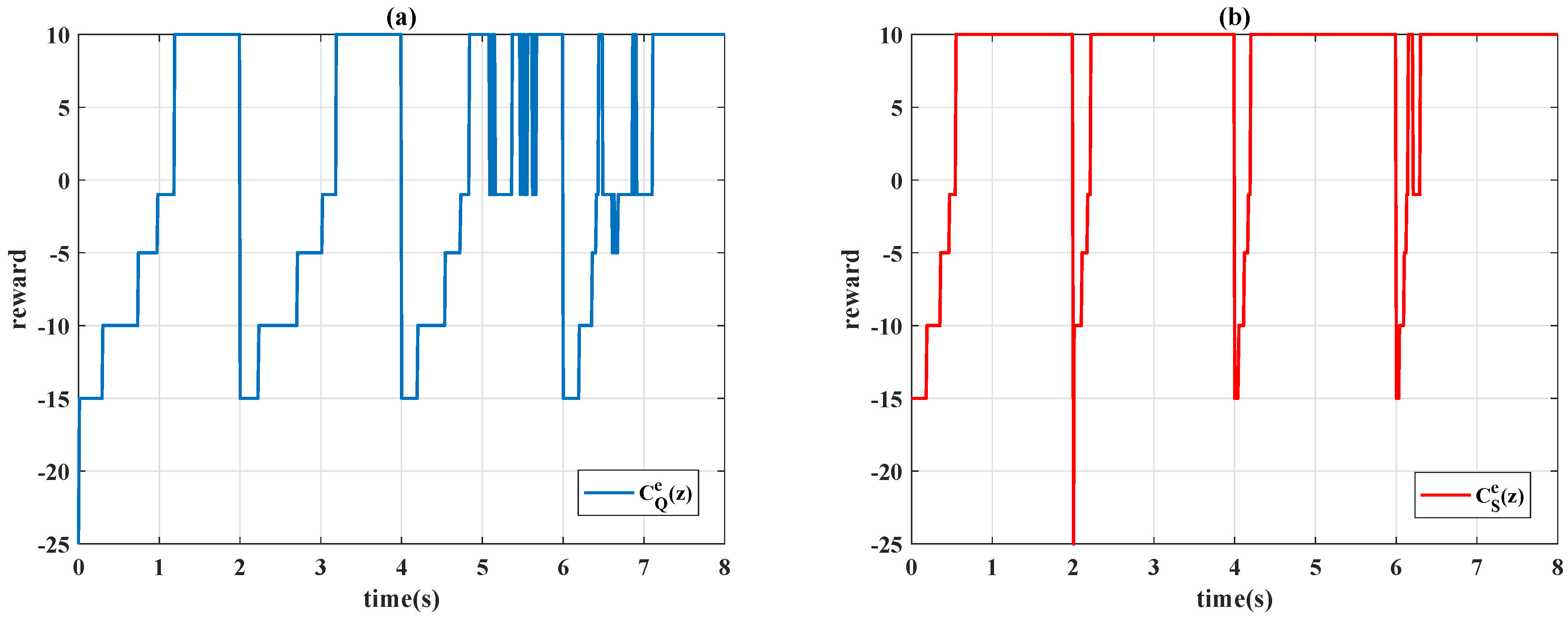
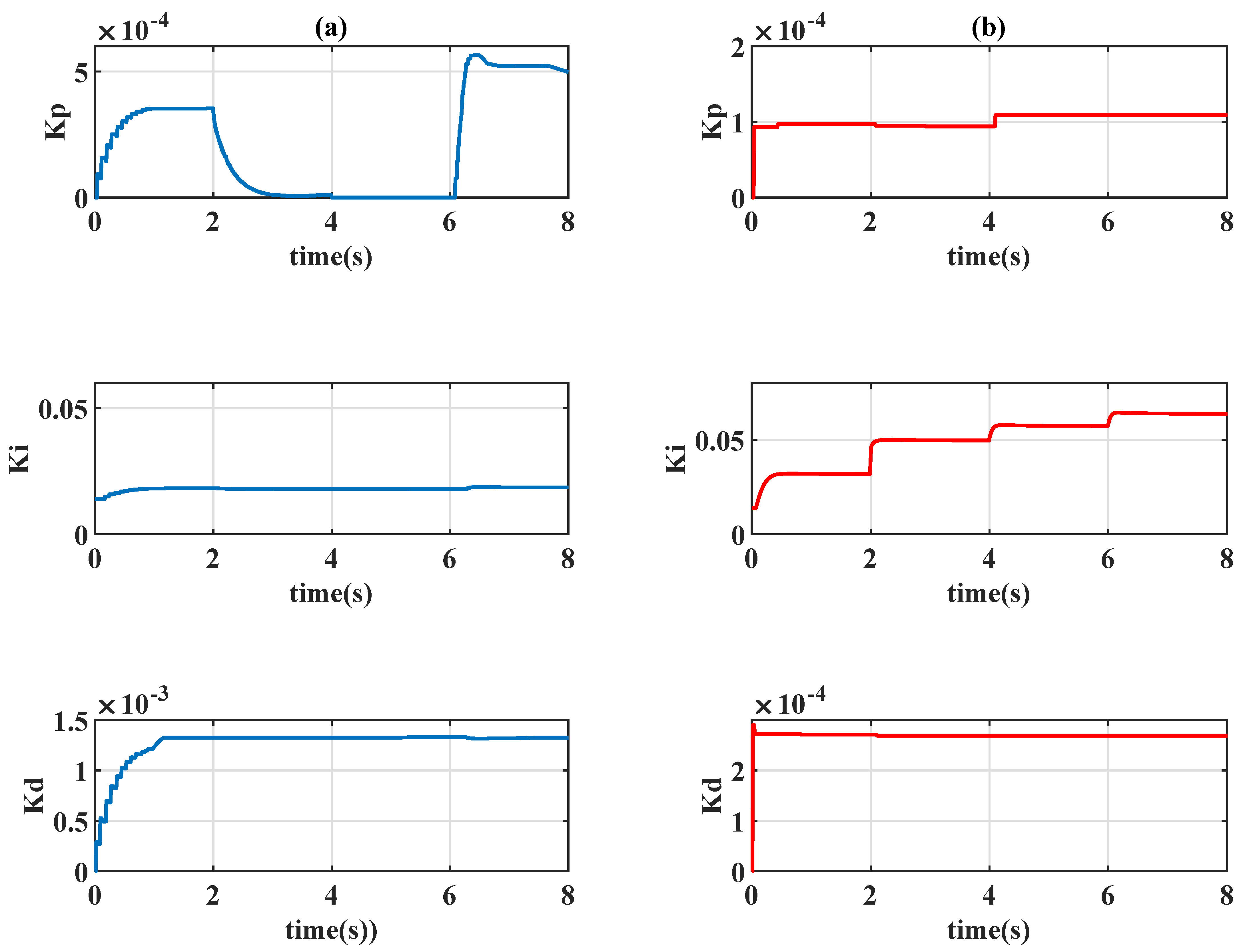
Remark 2.

In the conventional application of the reinforcement learning (see example 6.6 of [7]), the numerical value of reward is separately assigned for the gridworld example. The same concept is used in this paper to provide more degree-of-freedoms of adjustment; a partition error is consequently used instead of a continuous domain value as $R_t=\left|e_t\right|$.

In this paper, eight cases of action for the agent are examined, and the movement of the actions are detailed in

Table 2. Actions of the learning algorithm.

Action	Adjustment
1	if $|e_t| \ge$ 1, $K_i\leftarrow K_i+0.014$, else $K_i\leftarrow K_i+0.0014·p_t$
2	$K_p\leftarrow K_p-0.00002·p_t$
3	$K_d\leftarrow K_d+0.0003·p_t$
4	$K_i\leftarrow K_i-0.00002·p_t$
5	$K_p\leftarrow K_p+0.0001·p_t$
6	$K_d\leftarrow K_d-0.00002·p_t$
7	no action
8	$K_i\leftarrow K_i+0.00002·p_t$

, where $p_t$ is the scheduling variable [38] to be determined. According to the current value of the scheduling signal, the scheduling variable provides an additional chance for the agent to adapt to environmental changes. On the basis of these actions, the discrete time transfer function expression of the control law (4) is given as

$$\begin{array}{c}\hfill u_t=C(z,Q(S_t,A_t),p_t)e_t\end{array}$$

with the controller design

$$\begin{array}{c}\hfill C(z,Q(S_t,A_t),p_t)={\overline{K}}_p+{\overline{K}}_i\frac{z}{z-1}+{\overline{K}}_d\frac{z-1}{z},\end{array}$$

(5)

where the control gains ${\overline{K}}_p=K_p$, ${\overline{K}}_i=K_i\Delta t$, ${\overline{K}}_d=K_d/\Delta t$ are adjusted through the selected reinforcement learning algorithm $Q(S_t,A_t)$ and the scheduling variable $p_t$. The closed-loop control system structure is shown in Figure 4.

Remark 3.

In this paper, the only state S of Algorithms 1 and 2 is the error signal $e_t$; therefore, the condition "S is terminal" for the algorithms is naturally satisfied for each step, and only one decision is made for each episode since the concept of n-armed bandit is employed.

4. Experimental Results

The proposed control designs were tested along the x-direction of the piezo-actuated stage PI P-602.2CL; a data acquisition (DAQ) card NI PCIe-6346 was employed as an analog–digital interface; the analog I/O channels were arranged by an NI BNC-2110 shielded connector; the control signal was amplified by a PI E-503 amplifier before being fed to the piezoelectric transducer; and the system output displacement was measured and processed by a PI E-509.C3A signal conditioner.

4.1. Gain-Scheduled Actions

In the control stage, the initial value of the controller coefficients in (4) were set as $K_p=K_i=K_d=0$ with a sampling period $\Delta t=0.01$ s, the learning parameters of action value functions (1) and (3) are $\alpha =\gamma =0.99$, and $ϵ=0.021$ is specified for the $ϵ$-greedy policy (2). In this paper, two different scheduling variables $p_t$ in Table 2 were selected to reveal the effectiveness of gain-scheduled actions.

4.1.1. $p_t=1$

In this case, if the scheduling variable is set as $p_t=1$, the actions are unscheduled. Figure 5 depicts the step responses of the controller (5) with the different selected algorithms that form the Sarsa controller

$$\begin{array}{c}\hfill C_S^1\left(z\right)=C(z,Q_S(S_t,A_t),1)\end{array}$$

and the Q-learning controller

$$\begin{array}{c}\hfill C_Q^1\left(z\right)=C(z,Q_Q(S_t,A_t),1).\end{array}$$

Figure 6 presents the learning curves of different algorithms, Figure 7 presents the time history of the control gains, and Figure 8 presents the control signals. In Figure 5, Sarsa (red line) has a faster transient response (shorter rise time) but an undesirable overshoot and a longer settling time; Q-learning provides precise set-point performance with a shorter settling time, but the system output unpredictably jumps to an overshoot at $0.78$ s. At that moment, even if the system has been settled in a steady state, the control gains $K_p$ and $K_i$ are increased by Q-learning algorithm when the error signal is almost 0. Moreover, Q-learning had chattering between the first and third second because the control gains were switching rapidly, and Sarsa had a smoother response and a stable steady-state response.

4.1.2. $p_t=e_t$

In the previous unscheduled case, the controlled system was observed to have an unexpected overshoot during the steady state, and the output trajectory causes undesirable sharp corners and chattering. To eliminate these drawbacks, the scheduling variable of the actions is set as $p_t=e_t$, and the proposed controllers are as follows:

$$\begin{array}{c}\hfill C_S^e\left(z\right)=C(z,Q_S(S_t,A_t),e_t)\mathrm{and}{C}_Q^e\left(z\right)=C(z,Q_Q(S_t,A_t),e_t)\end{array}$$

(6)

The system responses of the proposed controllers are displayed in

Table 3. Statistical comparison of the controllers.

	Q-Learning Controller		Sarsa Controller
	${\mathit{C}}_{\mathit{Q}}^{\mathbf{1}}\left(\mathit{z}\right)$	${\mathit{C}}_{\mathit{Q}}^{\mathit{e}}\left(\mathit{z}\right)$	${\mathit{C}}_{\mathit{S}}^{\mathbf{1}}\left(\mathit{z}\right)$	${\mathit{C}}_{\mathit{S}}^{\mathit{e}}\left(\mathit{z}\right)$
Rise Time (s)	0.1226	0.1152	0.0559	0.0548
Settling Time (s)	6.142	0.2886	1.1533	0.1592
Overshoot (%)	15.6647	0.1838	14.4465	0.2477
RMSE (um)	0.4224	0.4026	0.3783	0.3652

and Figure 9. For the controller $C_Q^e\left(z\right)$ and $C_S^e\left(z\right)$, Figure 10 presents the learning curves, Figure 11 depicts the time-varying control gains, and Figure 12 shows the control signals. Figure 9 reveals that the gain-scheduled actions with $p_t=e_t$ improve system performance; the rising stage is similar to the unscheduled case $p_t=1$, but the undesirable overshoots are removed. The output trajectories are smoothed with the scheduling variable $p_t=e_t$ because the control gains in Figure 11 are almost constant during the steady state, and the learning curves in Figure 10 reveal that the learning algorithms always choose the case of $R_t=10$ when the system error $e_t$ converges to 0.

4.2. Comparison to Constant PID Controllers

For the purpose of comparison, different constant control designs are selected to present the obstacle of constant parameter choosing. The selected constant control gains are given in

Table 4. Controller gains of the constant PID controllers.

	${\mathit{C}}_1\left(\mathit{z}\right)$	${\mathit{C}}_2\left(\mathit{z}\right)$	${\mathit{C}}_3\left(\mathit{z}\right)$	${\mathit{C}}_4\left(\mathit{z}\right)$	${\mathit{C}}_5\left(\mathit{z}\right)$
$K_P$	0.000567	0.000371	0.022680	0.2	1.2
$K_I$	0.041982	0.056906	0.083964	0.083964	0.083964
$K_D$	0.00185	0.001085	0.074	0.074	0.074

, in which the coefficients of $C_1\left(z\right)$ and $C_2\left(z\right)$ are specified by the final value (control gains at system time $t\Delta t=4$ s) of $C_Q^e\left(z\right)$ and $C_S^e\left(z\right)$, respectively. Compare with the performance of time-varying controller $C_Q^e\left(z\right)$ and $C_S^e\left(z\right)$, system output performances of constant controllers are depicted in Figure 13. It is seen the transient performances of time-varying designs $C_Q^e\left(z\right)$ and $C_S^e\left(z\right)$ were significantly faster than that of the constant control design $C_1\left(z\right)$ and $C_2\left(z\right)$ with the same level of control gains, thus illustrating the advantages of the time-varying control design over the constant one. When the constant control gains are increased as $C_3\left(z\right)$, the output performance shows a slightly faster rise time, but still large settling time. When control gain $K_P$ is increased for controller $C_4\left(z\right)$, the system has a shorter rise time but slower settling time than $C_3\left(z\right)$, and the output signal begins to oscillate in the very initial time period. When the coefficient $K_P$ is further increased, the oscillation becomes serious and the undesirable overshoot occurs, the system performs relatively slow convergency with an extremely large control gain $K_P$. In this comparison, the experimental results show the time-varying control design improves both transient (rise time) and steady state (settling time) performance with relatively small control gains.

4.3. Time-Varying Reference

To provide a more complete set of validation experiments, the controllers (6), and $C_1\left(z\right)$, $C_2\left(z\right)$ in Table 4, are tested using a piecewise step function

$$\begin{array}{c}\hfill r_t=5\lceil \Delta t\frac{t}{2}\rceil ,\mathrm{where}t\in [0,800].\end{array}$$

(7)

In Figure 14, the time history of the system outputs is presented, and the control signals are shown in Figure 15. In Figure 14, it is seen that the time-varying controller $C_Q^e\left(z\right)$ and constant design $C_1\left(z\right)$ had similar behavior; the time-varying design only had a slight improvement in performance as the step function increased. By contrast, the time-varying Sarsa controller $C_S^e\left(z\right)$ exhibited considerable learning progress; the algorithm effectively compensated for the tracking error at the second step of (7). The accuracy of the positioning is further evident in Figure 16; the Sarsa controller drives the system output to gain an optimal reward most of time. As indicated in Figure 17, the Sarsa algorithm properly adjusts the controller parameter $K_i$ subject to the movement of the reference signal, whereas the Q-learning algorithm ignores the desired reference characteristic (7).

4.4. Robustness Test

To test the robustness of the proposed time-varying control design, an unknown disturbance is added to the control signal, and the control input becomes

$$\begin{array}{c}\hfill u_t=C(z,Q(S_t,A_t),p_t)e_t+d_t,\end{array}$$

where $d_t=sin(2\pi t\Delta t)$ is a sinusoidal external disturbance.

In Figure 18, the output responses are depicted, and Figure 19 shows the control signals of different controller designs. Figure 18 indicates the system performance has a smoother trajectory when the scheduling variable is specified as $p_t=e_t$, and the Sarsa-based designs $C_S^1\left(z\right)$ and $C_S^e\left(z\right)$ perform superior robustness to the unknown disturbance.

5. Conclusions

This paper presents a time-varying PID controller design in which the control gains are automatically adjusted by the reinforcement algorithms. The concept of the n-armed bandit problem was used to simplify the learning process. Different learning algorithms were applied to the control design, and the control performance was experimentally evaluated on a piezo-actuated stage. The results reveal the potential of the proposed controller for handling system nonlinearity; various performance requirements were met, and the gain-scheduled actions improved the steady-state response and smoothed the system output trajectory. Moreover, adaptability to a time-varying reference signal and unknown disturbance was demonstrated. The Sarsa controller effectively compensates for variation in the reference signal and unknown disturbance, and the characteristic of the reference signal was successively learned by the time-varying controller.

References

1. Rozlosnik, A.E. Reimagining infrared industry with artificial intelligence and IoT/IIoT. In Thermosense: Thermal Infrared Applications XLII. International Society for Optics and Photonic; SPIE Digital library: Buenos Aires, Argentina, 2020; Volume 11409. [Google Scholar]
2. Rathod, J. Branches in Artificial Intelligence to Transform Your Business! Medium.com. 24 November 2020. Available online: https://pub.towardsai.net/branches-in-artificial-intelligence-to-transform-your-business-f08103a91ab2 (accessed on 25 November 2021).
3. Simeone, O. A very brief introduction to machine learning with applications to communication systems. IEEE Trans. Cogn. Commun. Netw. 2018, 4, 648–664. [Google Scholar] [CrossRef] [Green Version]
4. Zhai, X.; Oliver, A.; Kolesnikov, A.; Beyer, L. S4L: Self-Supervised Semi-Supervised Learning. In Proceedings of the IEEE/CVF International Conference on Computer Vision, Seoul, Korea, 23 July 2019. [Google Scholar]
5. Wang, L. Discovering phase transitions with unsupervised learning. Phys. Rev. B 2016, 94, 195105. [Google Scholar] [CrossRef] [Green Version]
6. Herbrich, R. Learning Kernel Classifiers Theory and Algorithms; MIT Press: Cambridge, MA, USA, 2002. [Google Scholar]
7. Sutton, R.S.; Barto, A.G. Reinforcement Learning: An Introduction, 2nd ed.; MIT Press: Cambridge, MA, USA, 2014. [Google Scholar]
8. Watkins, C.J.C.H. Learning from Delayed Rewards; King’s College: Cambridge, UK, 1989. [Google Scholar]
9. Sutton, R.S. Temporal Credit Assignment in Reinforcement Learning. Doctoral Dissertation, University of Massachusetts Amherst, Amherst, MA, USA, 1985. [Google Scholar]
10. Sutton, R.S. Learning to predict by the methods of temporal differences. Mach. Learn. 1988, 3, 9–44. [Google Scholar] [CrossRef]
11. Rummery, G.A.; Niranjan, M. On-Line Q-Learning Using Connectionist Systems; University of Cambridge, Department of Engineering: Cambridge, UK, 1994. [Google Scholar]
12. Tavakoli, F.; Derhami, V.; Kamalinejad, A. Control of Humanoid Robot Walking by Fuzzy Sarsa Learning. In Proceedings of the 2015 3rd RSI International Conference on Robotics and Mechatronics (ICROM), Tehran, Iran, 7–9 October 2015; pp. 234–239. [Google Scholar]
13. Yuvaraj, N.; Raja, R.; Ganesan, V.; Dhas, S.G. Analysis on improving the response time with PIDSARSA-RAL in ClowdFlows mining platform. EAI Endorsed Trans. Energy Web 2018, 5, e2. [Google Scholar] [CrossRef] [Green Version]
14. Shi, Q.; Lam, H.K.; Xiao, B.; Tsai, S.H. Adaptive PID controller based on Q-learning algorithm. CAAI Trans. Intell. Technol. 2018, 3, 235–244. [Google Scholar] [CrossRef]
15. Hakim, A.E.; Hindersah, H.; Rijanto, E. Application of Reinforcement Learning on Self-Tuning PID Controller for Soccer Robot. In Proceedings of the Joint International Conference on Rural Information & Communication Technology and Electric-Vehicle Technology (rICT & ICeV-T), Bandung, Indonesia, 26–28 November 2013; pp. 26–28. [Google Scholar]
16. Koszałka, L.; Rudek, R.; Poz’niak-Koszałka, I. An Idea of Using Reinforcement Learning in Adaptive Control Systems. In Proceedings of the International Conference on Networking, International Conference on Systems and International Conference on Mobile Communication and Learning Technologie (ICNICONSMCL’06), Morne, Mauritius, 23–29 April 2006; p. 190. [Google Scholar]
17. Yang, Y.; Wan, Y.; Zhu, J.; Lewis, F.L. H Tracking Control for Linear Discrete-Time Systems: Model-Free Q-Learning Designs. IEEE Control. Syst. Lett. 2020, 5, 175–180. [Google Scholar] [CrossRef]
18. Sun, W.; Zhao, G.; Peng, Y. Adaptive optimal output feedback tracking control for unknown discrete-time linear systems using a combined reinforcement Q-learning and internal model method. IET Control. Theory Appl. 2019, 13, 3075–3086. [Google Scholar] [CrossRef]
19. Liu, Y.; Yu, R. Model-free optimal tracking control for discrete-time system with delays using reinforcement Q-learning. Electron. Lett. 2018, 54, 750–752. [Google Scholar] [CrossRef]
20. Fu, H.; Chen, X.; Wang, W.; Wu, M. MRAC for unknown discrete-time nonlinear systems based on supervised neural dynamic programming. Neurocomputing 2020, 384, 130–141. [Google Scholar] [CrossRef]
21. Radac, M.-B.; Lala, T. Hierarchical Cognitive Control for Unknown Dynamic Systems Tracking. Mathematics 2021, 9, 2752. [Google Scholar] [CrossRef]
22. Veselý, V.; Ilka, A. Gain-scheduled PID controller design. J. Process Control 2013, 23, 1141–1148. [Google Scholar] [CrossRef]
23. Poksawat, P.; Wang, L.; Mohamed, A. Gain scheduled attitude control of fixed-wing UAV with automatic controller tuning. IEEE Trans. Control. Syst. Technol. 2017, 26, 1192–1203. [Google Scholar] [CrossRef]
24. Mizumoto, M. Realization of PID controls by fuzzy control methods. Fuzzy Sets Syst. 1995, 70, 171–182. [Google Scholar] [CrossRef]
25. Mann, G.K.; Hu, B.-G.; Gosine, R.G. Analysis of direct action fuzzy PID controller structures. IEEE Trans. Syst. Man Cybern. Part B (Cybern.) 1999, 29, 371–388. [Google Scholar] [CrossRef]
26. Carvajal, J.; Chen, G.; Ogmen, H. Fuzzy PID controller: Design, performance evaluation, and stability analysis. Inf. Sci. 2000, 123, 249–270. [Google Scholar] [CrossRef]
27. Tang, K.-S.; Man, K.F.; Chen, G.; Kwong, S. An optimal fuzzy PID controller. IEEE Trans. Ind. Electron. 2001, 48, 757–765. [Google Scholar] [CrossRef] [Green Version]
28. Zhao, Z.-Y.; Tomizuka, M.; Isaka, S. Fuzzy gain scheduling of PID controllers. IEEE Trans. Syst. Man Cybern. 1993, 23, 1392–1398. [Google Scholar] [CrossRef] [Green Version]
29. Blanchett, T.; Kember, G.; Dubay, R. PID gain scheduling using fuzzy logic. ISA Trans. 2000, 39, 317–325. [Google Scholar] [CrossRef]
30. Bingul, Z.; Karahan, O. A novel performance criterion approach to optimum design of PID controller using cuckoo search algorithm for AVR system. J. Frankl. Inst. 2018, 355, 5534–5559. [Google Scholar] [CrossRef]
31. Jin, X.; Chen, K.; Zhao, Y.; Ji, J.; Jing, P. Simulation of hydraulic transplanting robot control system based on fuzzy PID controller. Measurement 2020, 164, 108023. [Google Scholar] [CrossRef]
32. Van, M. An enhanced robust fault tolerant control based on an adaptive fuzzy PID-nonsingular fast terminal sliding mode control for uncertain nonlinear systems. IEEE/ASME Trans. Mechatronics 2018, 23, 1362–1371. [Google Scholar] [CrossRef] [Green Version]
33. Berry, D.A.; Fristedt, B. Bandit Problems: Sequential Allocation of Experiments; Chapman and Hall: London, UK, 1985. [Google Scholar]
34. Dearden, R.; Friedman, N.; Russell, S. Bayesian Q-learning. In Aaai/iaai; American Association for Artificial Intelligence: Palo Alto, CA, USA, 1998; pp. 761–768. [Google Scholar]
35. Goldfarb, M.; Celanovic, N. Modeling piezoelectric stack actuators for control of micromanipulation. IEEE Control. Syst. Mag. 1997, 17, 69–79. [Google Scholar]
36. Yeh, Y.L.; Yen, J.Y.; Wu, C.J. Adaptation-Enhanced Model-Based Control with Charge Feedback for Piezo-Actuated Stage. Asian J. Control 2020, 22, 104–116. [Google Scholar] [CrossRef]
37. Åström, K.J.; Hägglund, T. Advanced PID Control; ISA—The Instrumentation, Systems, and Automation Society: Research Triangle Park, NC, USA, 2006. [Google Scholar]
38. Rugh, W.J.; Shamma, J.S. Research on gain scheduling. Automatica 2000, 36, 1401–1425. [Google Scholar] [CrossRef]
Figure 1. Agent–environment interface [7].
Machines 09 00319 g001
Figure 2. Model of a piezoelectric transducer.
Machines 09 00319 g002
Figure 3. Block diagram of a piezo-actuated stage [36].
Machines 09 00319 g003
Figure 4. Closed-loop control system structure.
Machines 09 00319 g004
Figure 5. Step responses with p t = 1 .
Machines 09 00319 g005
Figure 6. Learning curves with p t = 1 : (a) Q-learning C Q 1 ( z ) ; (b) Sarsa C S 1 ( z ) .
Machines 09 00319 g006
Figure 7. Time-varying gains of PID controllers with p t = 1 : (a) Q-learning C Q 1 ( z ) ; (b) Sarsa C S 1 ( z ) .
Machines 09 00319 g007
Figure 8. Control signals with p t = 1 : (a) Q-learning C Q 1 ( z ) ; (b) Sarsa C S 1 ( z ) .
Machines 09 00319 g008
Figure 9. Step responses: (a) Q-learning; (b) Sarsa.
Machines 09 00319 g009
Figure 10. Learning curves with p t = e t : (a) Q-learning C Q e ( z ) ; (b) Sarsa C S e ( z ) .
Machines 09 00319 g010
Figure 11. Time-varying gains of PID controllers with p t = e t : (a) Q-learning C Q e ( z ) ; (b) Sarsa C S e ( z ) .
Machines 09 00319 g011
Figure 12. Control signals with p t = e t : (a) Q-learning C Q e ( z ) ; (b) Sarsa C S e ( z ) .
Machines 09 00319 g012
Figure 13. Output responses of constant PID controllers.
Machines 09 00319 g013
Figure 14. Output responses of: (a) Q-learning controllers; (b) Sarsa controllers.
Machines 09 00319 g014
Figure 15. Control signals: (a) Q-learning C Q e ( z ) and C Q f ( z ) ; (b) Sarsa C S 1 ( z ) and C S f ( z ) .
Machines 09 00319 g015
Figure 16. Learning curves of: (a) Q-learning C Q e ( z ) ; (b) Sarsa C S e ( z ) .
Machines 09 00319 g016
Figure 17. Time-varying gains of PID controllers of (a) Q-learning C Q e ( z ) and (b) Sarsa C S e ( z ) .
Machines 09 00319 g017
Figure 18. Output responses of: (a) Q-learning controllers; (b) Sarsa controllers.
Machines 09 00319 g018
Figure 19. Control signals: (a) Q-learning C Q e ( z ) and C Q 1 ( z ) ; (b) Sarsa C S Q ( z ) and C S 1 ( z ) .
Machines 09 00319 g019