PMSM Speed Control Based on Particle Swarm Optimization and Deep Deterministic Policy Gradient under Load Disturbance

Abstract

Proportional integral-based particle swarm optimization (PSO) and deep deterministic policy gradient (DDPG) algorithms are applied to a permanent-magnet synchronous motor to track speed control. The proposed methods, based on notebooks, can deal with time delay challenges, imprecise mathematical models, and unknown disturbance loads. First, a system identification method is used to obtain an approximate model of the motor. The load and speed estimation equations can be determined using the model. By adding the estimation equations, the PSO algorithm can determine the sub-optimized parameters of the proportional-integral controller using the predicted speed response; however, the computational time and consistency challenges of the PSO algorithm are extremely dependent on the number of particles and iterations. Hence, an online-learning method, DDPG, combined with the PSO algorithm is proposed to improve the speed control performance. Finally, the proposed methods are implemented on a real platform, and the experimental results are presented and discussed.

1. Introduction

Motors are widely utilized as the main power source in modern industries, and can be roughly classified into two types: direct current (DC) and alternating current (AC) motors. DC motors operate on the principle of basic magnetism, and the speed and torque are easy to control; however, DC motors have the disadvantages of high operation and maintenance costs. Furthermore, DC motors cannot operate under explosive and hazardous conditions because sparking occurs at the brush. Currently, AC motors are more widely utilized in industrial applications. AC motors can be classified into two parts: induction motors [1] and synchronous motors [2]. This study analyzes permanent magnet synchronous motors (PMSMs). Because of the advantages of high power density, high reliability, and low motor volume, PMSMs are used in computer numerical control (CNC) machines, electric vehicle drive systems, and robots. Field-oriented control (FOC) [3] is a popular strategy for controlling AC motors. FOC decouples the torque and flux by transforming the stationary phase currents to a rotating d-q frame. By using the FOC method, the AC motor control challenge can be simplified to a DC motor control challenge.

The control accuracy of the motor directly affects the performance of the system. The literature [4] indicates that the rotation speed and propulsive force are two important parameters in an air-borne bolting system. The breakage of the drill pipe and the inability of the drill bit to cut the coal adequately can be caused by the unreasonable rotation speed and propulsive force. In [5], it was found that, to produce precision parts, precise rotational accuracy and a constant machine tool spindle speed are required. However, inevitable changes in the spindle speed caused by the cutting force will lead to low-quality surfaces. In addition, the rotation speed of the pin tool is an important controlled variable in friction stir welding machines [6]. By controlling the rotating speed, a constant vertical force is obtained during the welding process.

Generally, the proportional derivative (PD), proportional-integral (PI), and proportional-integral-derivative (PID) are the most common controllers used to design the control system [7,8]. In addition, a few studies have proposed alternative algorithms for motor speed control. The literature [9] proposes an on-line tuning fuzzy proportional derivative controller based on the equivalent errors to deal with the contouring control of robot manipulators. The results show that the controller can effectively deal with highly non-linear dynamic systems following an analytic/non-analytic path. A hybrid fuzzy-PI controller is proposed to address the challenges of chattering effects and large execution times [10]. Nonlinear controllers such as feedback linear control [11], sliding mode control [12], and adaptive control [13] are presented. In addition, model prediction control has been successfully used for the current and torque control of motors [14,15]. However, the aforementioned algorithms require precise knowledge of the nonlinear model of the motor, which is difficult to obtain.

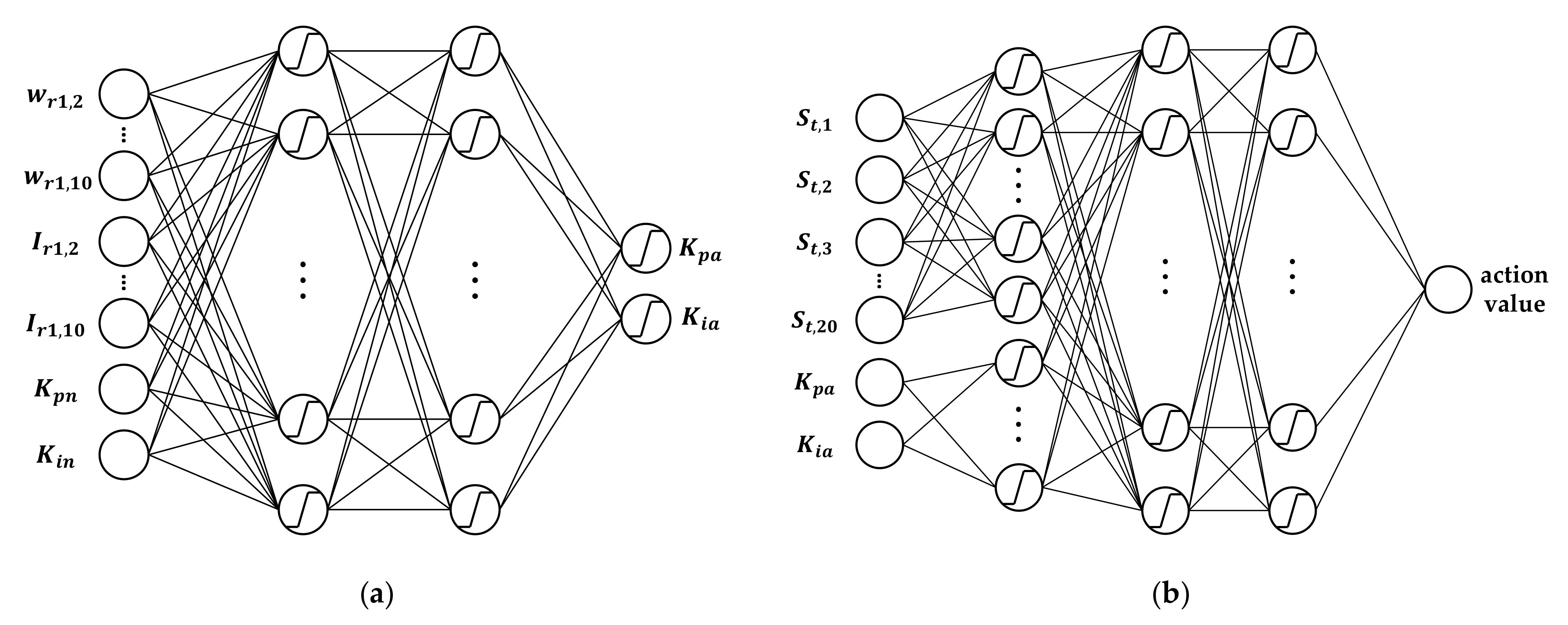
This study adopts the particle swarm optimization (PSO) and deep deterministic policy gradient (DDGP) algorithms to address the motor speed tracking challenge. In 1995, the PSO algorithm was proposed by Kennedy and Eberhart [16]. The PSO algorithm is inspired by the intelligent collective behavior of some animals, and is initialized with a group of random particles, where each individual particle represents a single solution. The particles move through the search space to obtain the optimized solution. The movement direction and velocity of the particles are updated according to the local and global best solutions. Numerous studies have indicated that the PSO algorithm is a powerful optimization method used in various applications. In [17], a learning model is used to determine the distance between the mobile sensor node and the anchor node. A PSO-based artificial neural network is proposed to improve the estimation accuracy. In contrast to the conventional optimization method of feed-forward backpropagation, PSO is utilized to update the weights of the network. In [18], a PSO-based PID controller is proposed to address the position control of the hydraulic system. The PSO algorithm is utilized to tune the parameters of the PID controller, and the results indicate that the rising time, settling time, and integral time absolute error can be reduced. The literature [19] reveals that the PSO algorithm can also be implemented in the field of control. In [19], a PSO-IAC algorithm, integrated by the adaptive inertia weight and constriction factor, is proposed to increase the convergence velocity. The results indicate that the challenge of reaching the avoidance problem can be addressed. A PSO, combined with a radial basis function neural network, is proposed to deal with the pitch control of a wind turbine [20]. In addition, a graphical approach is utilized to visualize the 2D or 3D boundaries of the PID controller. Under the delay time effects, the stochastic inertia weight PSO can effectively handle pitch control.

Recently, machine learning has become a popular technique. Generally, unsupervised learning [21], supervised learning [22], and reinforcement learning [23] are the three main types of machine learning strategies. First, unsupervised learning is typically utilized in the fields of data clustering and dimensionality reduction. It does not require a complete and clean labeled dataset, such as principle component analysis [24], autoencoder [25], and t-SNE [26]. Supervised learning deals mainly with classification and regression problems. It requires well-labelled dataset, such as a convolutional neural network [27], long short-term memory [28], and random forest [29]. In addition, in the literature [30], a two-layer recursive neural network was used to approximate a motor model, and the network was considered to be a motor speed predictor.

Reinforcement learning is a framework for learning the relationship between states and actions. Ultimately, the agent can maximize the expected reward and learn how to complete a mission. Q-learning [31] and deep Q network (DQN) [32] are common value-based reinforcement learning algorithms. The policy usually takes the largest action with the largest action value. For the DQN, the Q table is replaced by a deep neural network to estimate the action value. Experience replay is utilized to break the correlations between the samples, which prevents the agent from overfitting to the sequence of training. In [33], unlike the conventional control method, the complex nonlinear model of the PMSM does not need to be known. A DQN-based controller is proposed to control the direct torque of the PMSM; however, DQN can only deal with discrete and low-dimension action spaces. In contrast to value-based learning, policy-based learning uses a stochastic policy that gives the probability of action in a specific state. The policy gradient [34] is a basic policy-based learning algorithm. The advantage of policy-based learning is that it can effectively deal with high-dimensional and continuous action spaces; however, the learning methods tend to converge to the local optima. To improve the performance of reinforcement learning, DDPG [35], TD3 [36], and SAC [37], combining Q-learning and policy gradient algorithms, are proposed. In [38], DDPG is used to solve the road-keeping challenge. The agent can determine the steering angle of the vehicle by observing the distance between the vehicle and the road boundaries. In [39], an optimal torque distribution control for multi-axle electric vehicles with in-wheel motors is proposed. The DDPG algorithm can optimize the drive torque for each motor to reduce the energy consumption of the vehicle.

The contributions of this paper are as follows:

• This paper proposes an online-learning DDPG with the PSO method to control the motor speed under a load disturbance.
• The PSO algorithm is used to find a sub-optimized solution of the PI controller using an approximate motor model. To safely train the model online and converge faster, the sub-optimized solutions are added into the policy function of the DDPG as a constraint.
• The proposed network is a model-free method; hence, a precise mathematical model of the motor is not required for speed control.
• The proposed model can deal with the delay problem as well.

The experimental results demonstrate that the proposed method can effectively reduce the settling time and overshoot of the speed response when a load disturbance occurs. Furthermore, the results indicate that the proposed method performs better than the conventional PSO and PI controllers.

The remainder of this paper is organized as follows. Section 2 presents the structure of the motor testing platform. Section 3 describes the methodology, in which the formulation and implementation of the system and reinforcement learning solution are discussed in detail. In Section 4, the experimental results obtained from a real platform are presented. The experimental results indicate that the proposed method can effectively handle speed tracking control. Section 5 concludes this study.

2. Motor Testing Platform

In this study, the motor testing platform illustrated in Figure 1 was built. The motor testing platform comprised two PMSMs and one speed sensor. The analyzed PMSM was ECM-A3L-0807, developed by Delta Electronics. The rated speed and torque of the motor are 2.39 Nm and 3000 rpm, respectively. The speed sensor used was DATAFLEX^® 16, which was manufactured by KTR Systems GmbH. The speed sensor outputs a voltage ranging from 0 to 10 V, and the maximum measured speed can be set from 10 to 10,000 rpm. The Hall sensor, ACS711EX, can handle bidirectional currents from −31 to +31 A with a 100 kHz bandwidth. The data acquisition unit used was USB-2405, manufactured by ADLINK Technology. It utilizes the 24-bit Sigma-Delta ADC with a built-in 165 anti-aliasing filter and four simultaneous sampling analog input channels up to 128 kS/s.

As illustrated in Figure 1, the two motors were mounted on the motor testing platform. Motor I was set in speed control mode and was controlled at a constant speed, Motor II was set in torque control mode, and it could provide instant and inversed torque as a disturbance. This study utilized a notebook as the computational platform, and it communicated to the actuator through RS-485. The speed sensor was connected between the two motors to measure the rotating speed of Motor I. Three Hall sensors were individually clamped to the three-phase wires of Motor I. To acquire a more stable current signal, the power supplier was utilized to feed a power of 5 V to the Hall sensors. Four signals were acquired by USB-2405, including the three-phase current signals and the speed signal of Motor I. The sampling rate was 4000 Hz. When the direction of the torque was opposite to the direction of rotation, the energy generated returned to the servo drive from the load. A regenerative resistor with 60 Ohm and 1000 Watt was used to consume the energy. Important peripheral devices are illustrated in Figure 2.

The computer used for training in this work was a notebook equipped with an NVIDIA GeForce GTX 1050 Ti and an Intel^® Core™ I7-8750H. The notebook had an 8G memory. This work used Python as a development tool owing to its convenient libraries, such as Keras and TensorFlow. C++ was used for human interface design. The drawings in this article were produced in MATLAB owing to the convenient drawing functions and esthetics of its figures.

3. Methods

This section describes the proposed speed control methods. Three methods were analyzed in this study including the fixed method, PSO algorithm, and DDPG. For the fixed method, the Delta actuator has a function that can provide the parameters of PI controller based on motor status and the settings in the actuator. However, the value does not change when the external load happens. For the PSO algorithm, the approximate model of the motor should be determined using the system identification method. Subsequently, the load and speed estimation equations are derived; however, the approximate models of the PI controller and motor cannot fully describe the real platform. Using both estimation equations, PSO can solely determine the sub-optimized values of $K_p$ and $K_i$ for the PI controller. Hence, the proposed method, which combines the DDPG and PSO, was used to learn the optimized solution online. The advantage of DDPG is that the method is a model-free algorithm. The performance of the proposed method is discussed in Section 4.

3.1. System Description

Figure 3 illustrates a control block diagram of the motor speed control system. $C\left(s\right)$ and $G\left(s\right)$ are the PI current controller and motor model, respectively. $w^{*}$ and $w$ are the speed command and output speed, respectively. $t_c$ is the torque command obtained by multiplying the torque constant $K_t$ by the current $i$. $t_L$ is the external load disturbance. Using the system identification methods proposed in [40,41], the estimation model is a second-order transfer function $G\left(s\right)$, as follows:

$$G\left(s\right)=\frac{W\left(s\right)}{T_c\left(s\right)-T_L\left(s\right)}=\frac{D}{A{s}^2+Bs+C}$$

(1)

The PI controller has the following form:

$$C\left(s\right)=\frac{K_{p}s+K_p{K}_i}{s}$$

(2)

where $K_p$ and $K_i$ are the proportional and integral gains.

Figure 3. Control block diagram of the motor speed control system.

Figure 3. Control block diagram of the motor speed control system.

3.2. Load and Speed Estimation Equation

In the analysis of the methods, unknown external load was seen as a disturbance to the system, which can cause the motor speed response to change. The load estimation equation was derived to estimate the unknown disturbance. Furthermore, a speed estimation equation was derived. Both estimation equations were adopted for predicting the speed response and to enable the PSO algorithm to determine the sub-optimized solution.

3.2.1. Load Estimation

According to Equation (1), the external load can be expressed as follows:

$$T_L\left(s\right)=T_c\left(s\right)-\frac{1}{D}\left(A{s}^2+Bs+C\right)W\left(s\right)$$

(3)

taking the inverse Laplace transform and assuming that the initial condition is zero. Then, the following differential equation can be obtained:

$$t_L\left(t\right)=t_c\left(t\right)-\frac{1}{D}\left(A\ddot{w}\left(t\right)+B\dot{w}\left(t\right)+Cw\left(t\right)\right)$$

(4)

Subsequently, the load estimation equation can be obtained by discretizing Equation (4).

$$t_L\left(k-1\right)=K_{t}i\left(k-1\right)-\frac{1}{D}\left(A\frac{w\left(k+1\right)-2w\left(k\right)+w\left(k-1\right)}{T_s^2}+B\frac{w\left(k\right)-w\left(k-1\right)}{T_s}+Cw\left(k-1\right)\right)$$

(5)

where $T_s$ is the sampling time.

3.2.2. Speed Estimation

Figure 3 illustrates that the transfer function $I\left(s\right)/E\left(s\right)=\left(K_{p}s+K_p{K}_i\right)/s$. Assume that the state $X\left(s\right)=E\left(s\right)/s$, and the differential equation is $\dot{x}\left(t\right)=e\left(t\right)$. $I\left(s\right)$ can be expressed as:

$$I\left(s\right)=K_{p}E\left(s\right)+K_p{K}_{i}X\left(s\right)$$

(6)

Taking the inversed Laplace transform, the current response is expressed as follows:

$$i\left(t\right)=K_{p}e\left(t\right)+K_p{K}_{i}x\left(t\right)$$

(7)

For the speed estimation equation, Equation (4) can be rewritten in the form

$$\ddot{w}\left(t\right)+\frac{B}{A}\dot{w}\left(t\right)=\frac{1}{A}\left(D\left(t_c\left(t\right)-t_L\left(t\right)\right)-Cw\left(t\right)\right)$$

(8)

Finally, the difference equations of Equation (7) is expressed as:

$$i\left(k\right)=K_p\left(w^{*}\left(k\right)-w\left(k\right)\right)+K_p{K}_{i}x\left(k\right)$$

(9)

and the speed estimation equation is

$$w\left(k+1\right)=2w\left(k\right)-w\left(k-1\right)-\frac{B}{A}\left(w\left(k\right)-w\left(k-1\right)\right)T_s+\left(\frac{D}{A}\left(t_c\left(k-1\right)-t_L\left(k-1\right)\right)-\frac{C}{A}w\left(k-1\right)\right)T_s^2$$

(10)

3.3. Particle Swarm Optimization Algorithm

In this study, the PSO algorithm was used to determine the parameters of PI controller. When a load is added into the motor system and the speed of the motor is significantly changed, the PSO algorithm starts. Figure 4 illustrates the operation of the PSO algorithm.

Figure 5 illustrates a general flowchart of the PSO algorithm. First, the number of PSO particles and dimension of the search space should be determined. At the $i_{th}$ iteration, the position and velocity of the particles can be expressed as follows:

$$X_n\left(i\right)=\left[x_{n1}\left(i\right), x_{n2}\left(i\right),\cdots , x_{nd}\left(i\right)\right], n=1,\dots ,m,$$

(11)

$$V_n\left(i\right)=\left[v_{n1}\left(i\right), v_{n2}\left(i\right),\cdots , v_{nd}\left(i\right)\right], n=1,\dots ,m,$$

(12)

where $X_n\left(i\right)$ represents the $n_{th}$ particle position and $V_n\left(i\right)$ is the $n_{th}$ particle velocity. $m$ and $d$ are the number of particles and dimension of the searching space, respectively. The individual best position $P_n$ and global best position $P_g$ are expressed as follows:

$$P_n\left(i\right)=\left[p_{n1}\left(i\right), p_{n2}\left(i\right),\cdots , p_{nd}\left(i\right)\right], n=1,\dots ,m,$$

(13)

$$P_g\left(i\right)=\left[p_{g1}\left(i\right), p_{g2}\left(i\right),\cdots , p_{gd}\left(i\right)\right], n=1,\dots ,m,$$

(14)

The integral absolute error (IAE), integral square error (ISE), integral time absolute error (ITAE), integral time square error (ITSE), and integral square time error (ISTE) are popular objective functions [42,43,44]. In this study, the IAE was adopted as the fitness function, which is calculated as follows:

$$T_{IAE}={{\displaystyle \sum }}_{k=1}^N\left|w^{*}\left(k\right)-w\left(k\right)\right|$$

(15)

where $T_{IAE}$ indicates the IAE value. The load disturbance is first estimated by the load estimation equation. Afterward, $N$ sampling points are predicted by the speed estimation equation for calculating the fitness function. Then, $T_{IAE}$ is calculated by subtracting the command speed and the estimated speed. By operating the following equations, the updated velocity and position of the particle can be obtained:

$$V_n\left(i+1\right)=w_p{V}_n\left(i\right)+C_1{R}_1\left(P_n\left(i\right)-X_n\left(i\right)\right)+C_2{R}_2\left(P_g\left(i\right)-X_n\left(i\right)\right)$$

(16)

$$X_n\left(i+1\right)=X_n\left(i\right)+V_n\left(i+1\right)$$

(17)

where $w_p$ is the inertia weight, which is a constant value. $C_1$ and $C_2$ are the individual and global coefficients, respectively. $R_1$ and $R_2$ are random numbers generated from a uniform distribution in the interval [−1, 1]. When the number of iterations is larger than the number of maximum iterations, the PSO algorithm stops.

In this study, the parameter settings of the PSO algorithm are shown in

Table 1. Parameter settings of the PSO algorithm.

Parameters	$\mathit{d}$	${\mathit{w}}_{\mathit{p}}$	${\mathit{C}}_1$	${\mathit{C}}_2$	$\mathit{N}$
Values	2	0.5	1.2	1.2	300

. The dimension of the searching space is 2 for $K_p$ and $K_i$. Furthermore, the number of the predicted sampling point is 300, about 0.075 s. Two settings of the maximum iteration number are discussed in Section 4.2.

3.4. Deep Deterministic Policy Gradiend with Particle Swarm Optimization

This study proposes a DDPG model to implement the online learning of speed tracking control. By combining the sub-optimized solutions of the PSO algorithm, the DDPG model can converge faster.

3.4.1. State-Space

The state space denotes observations from the environment. To train the model efficiently, the state variables should be strongly related to actions. According to the load estimation and speed estimation equations shown in Equations (5) and (10), the variations in the speed and current are important. In addition, the current values of $K_p$ and $K_i$ affect the compensatory performance of the current. To ensure the scales of each feature are similar, the values of $K_p$ and $K_i$ should be normalized to $K_{pn}$ and $K_{in}$. The normalization process is as follows:

$$K_{*n}=\frac{K_{*}}{S_{n*}}$$

(18)

$K_{*}$ indicates the values and of $K_p$ and $K_i$. $S_{n*}$ represents the space size of the $K_p$ and $K_i$. In this study, $S_{np}$ and $S_{ni}$ were 250 and 100, respectively. $K_{pn}, K_{in}$, and the amount of change of these two signals are measured and processed as the input state vectors.

Once the speed is continuously lower than $S_e$% of the command speed for $N_e$, with more than 9 sampling points, the tuning starts. The speed $W_r$ (rad/s) and current $I_r$ (A) signals in the $N_e$ continuous sampling points can be expressed as follows:

$$W_r=\left[w_{r1},w_{r2},\dots ,w_{r{N}_e}\right]$$

(19)

$$I_r=\left[i_{r1},i_{r2},\dots ,i_{r{N}_e}\right]$$

(20)

Figure 6 illustrates the measured signals for $W_r$ and $I_r$. By subtracting the first variable from the others and combining the two vectors, the input state vector $s_t$ can be obtained.

$$s_t=\left[w_{r1,2},w_{r1,3},\dots ,w_{r1,10},i_{r1,2},i_{r1,3},\dots ,i_{r1,10}, K_{pn}, K_{in}\right]$$

(21)

3.4.2. Action Space

The main actions controlling the speed response are the parameters of $K_p$ and $K_i$. The available setting ranges of $K_p$ and $K_i$ for the actuator utilized in this study are [0, 500] and [0, 100], respectively. However, by observing the sub-optimized solution solved by the PSO method, the boundary of $K_p$ can be restricted to [251, 500], and the setting range of $K_i$ is kept the same.

3.4.3. Reward Function Design

This study proposes a reward function that enables the agent to track the speed command. It encourages the agent to decrease the settling time and minimize the change in speed while the load disturbance occurs. The IAE of the speed response is a key measurement of how well the motor speed is maintained. Furthermore, to decrease the training time and protect the mechanism during online training, the sub-optimized solutions of $K_{ps}$ and $K_{is}$ are considered. Assume that the actions determined by the actor network are $K_{pa}$ and $K_{ia}$. In addition, the two search boundaries of the two actions are defined as $[D_{pl}$,$D_{pu}]$ and $\left[D_{il}, D_{iu}\right]$. The reward function $R$, based on the IAE and PSO, is presented as follows:

$$\left\{\begin{array}{c}r\left(s_t,a_t\right)=r_1\left(2e^{\left(r_2\frac{I}{I_n}\right)}-r_3\right), \mathrm{if} D_{*l}\le a_{*,t}\le D_{*u}] \\ r_t\left(s_t,a_t\right)=Q(s_t,a_t|{\theta }^Q)-0.1, \mathrm{otherwise}\end{array},\right.$$

(22)

where $r_1$ is a constant adopted to scale up the reward, and the neural network is allowed to converge more easily. The value of $r_1$ depends on the size of the action space. When the size of the action space is large, the value of $r_1$ should increase, otherwise, its value should decrease. $r_2$ is the decay rate, which is a negative constant. The normalized process is usually used in the reward function design [45,46,47], and is calculated by $I_w/I_n$. $I_w$ is the IAE value obtained by subtracting the command speed and the measured output speed. The number of the calculated sampling points is 300. $I_n$ is the average IAE result under a fixed $K_p$ and $K_i$. The fixed values of $K_p$ and $K_i$ are 226 and 36, respectively, which are calculated from the Delta actuator under the auto-tuning mode. $r_3$ is also a constant, which makes $r\cong 0.0$ when $I/I_n$ is 0.5. The design of $r_3$ leads the reward function to contain both positive and negative value. $D_{pu}$ and $D_{pl}$ are calculated as $K_{ps}\pm d_p$. Similarly, $D_{iu}$ and $D_{il}$ are calculated as $K_{ps}\pm d_i$. If action $a_{*,t}$ is out of the boundaries of $[D_{*l}$,$D_{*u}]$, a small punishment is given. Based on numerous experimental results and observations, the values of the parameters are shown in

Table 2. Parameter settings of the reward function.

Parameters	${\mathit{r}}_1$	${\mathit{r}}_2$	${\mathit{r}}_3$	${\mathit{d}}_{\mathit{p}}$	${\mathit{d}}_{\mathit{i}}$	${\mathit{I}}_{\mathit{n}}$
Values	10	−2.5	0.3	40	30	9000

.

3.4.4. Network Architecture

To determine the actions and evaluate the value of actions under a certain state, a critic network $Q(s,a|{\theta }^Q)$ and an actor $\mu (s|{\theta }^{\mu })$ were designed. The architectures of the networks are constructed by the fully connected layers, which are illustrated in Figure 7. After the experimental tuning, the proposed actor has one input state, as shown in Equation (21), including the values of $K_{pn}$ and $K_{in}$ and variations in the speed and current signals. Subsequently, two fully connected layers are connected. Finally, two output layers with the Tanh activation function generate the actions $K_{pa}$ and $K_{ia}$, which are in the range of −1 to 1. By scaling into the range of each action space, as mentioned in Section 3.4.2, the final actions can be obtained.

In addition, the proposed critic network has two input vectors including the state vector $s_t$ and the action vector. First, the two input vectors are connected to two fully connected layers separately, and are then concatenated together. Subsequently, one fully connected layer is connected. Finally, one linear output layer outputs the action value. All the fully connected layers used in the hidden layers are used with the ReLU [48] activation function. Adam optimization with the mean square error function is used to train the critic network. The mean of value given by the critic network is used to train the actor. Based on the tuning results, a fixed learning rate of 0.003 is assigned.

Table 3. Hyperparameter settings of the proposed actor network.

Size of the input state	$20\times 1$
Input size of the 1st fully connected layer	$20\times 1$
Input size of the 2nd fully connected layer	$256\times 1$
Input size of output layer	$256\times 1$
Output size of output layer	$2\times 1$
Learning rate	$0.003$

and

Table 4. Hyperparameter settings of the proposed critic network.

Size of the state vector	$20\times 1$
Size of the action vector	$2\times 1$
Input size of the 1st fully connected layer	$20\times 1$
Input size of the 2nd fully connected layer	$2\times 1$
Input sizes of the concatenate layer: (1st fully connected layer) (2nd fully connected layer)	$48\times 1$ $48\times 1$
Input size of the 3rd fully connected layer	$96\times 1$
Input size of the 4th fully connected layer	$256\times 1$
Input size of output layer	$256\times 1$
Output size of output layer	$1\times 1$
Learning rate	$0.003$

list the hyperparameter settings of the proposed critic and actor networks.

The details of the reinforcement motor speed control method are presented in Algorithm 1. First, the experience memory $M$ with the size of 100, and the critic, actor, and target networks are initialized. Afterward, every 5 s, motor II changes the disturbance load in the range of 0.0 to 1.0 Nm. If significant change happens on the motor speed, the state $s_t$ is fed into the actor and determines the parameter settings of PI controller. The exploration noise ${ϵ}_t$ is a random number, which is in the range of −5.0–5.0 after scaling. The reward is calculated after the actions are implemented on the motors. Then, the critic, actor, and target networks are updated. $\mathsf{\tau }$ denotes the changed rate of the target network. The design of $\mathsf{\tau }$ is intended to change the weight of the target network slowly, which is 0.05 in this paper.

Algorithm 1 DDPG for Speed Tracking Control

1: Initialize experience memory $M$

2: Randomly initialize critic network $Q(s,a|{\theta }^Q)$ and actor $\mu (s|{\theta }^{\mu })$ with weights ${\theta }^Q$ and ${\theta }^{\mu }$

3: Initialize target network $Q^{\prime }$ and ${\mu }^{\prime }$ with weights ${\theta }^{Q^{\prime }}\leftarrow {\theta }^Q$, ${\theta }^{{\mu }^{\prime }}\leftarrow {\theta }^{\mu }$

4: repeat

5: Randomly select disturbance load in the range of 0.0~1.0 Nm

6: if significant change in motor speed then

7: Observe the state $s_t$, and calculate sub-optimized solutions and boundaries $K_{ps}$, $K_{is}$, $D_{pl}$, $D_{pu}$, $D_{il}$, and $D_{iu}$

8: Select the actions $a_t=\mu \left(s_t|{\theta }^{\mu }\right)+{ϵ}_t$ according to the current policy and exploration noise

9: if$a_{*,t}$ is out of the boundaries of $[D_{*l}$$,D_{*u}]$ then

a. Store transition $\left(s_i,a_i,r_i\right)$

b. Randomly select action $a_{*,t}$ in the boundary of $[D_{*l}$$,D_{*u}]$

10: end if

11: Execute actions $a_t$ and observe reward $r_t$

12: Store transition $\left(s_i,a_i,r_i\right)$

13: Sample a random minibatch of ${\mathrm{N}}_m$ transitions $(s_i,a_i,r_i)$ from $M$

14: Set $y_i=r_i$

15: Update critic by minimizing the loss $L=\frac{1}{{\mathrm{N}}_m}{{\displaystyle \sum }}_i{(y_i-Q(s_i,a_i|{\theta }^Q))}^2$

16: Update the actor policy using the sampled policy gradient:

17:  ${\nabla }_{{\theta }^{\mu }}J\approx \frac{1}{{\mathrm{N}}_m}{{\displaystyle \sum }}_i{\nabla }_{a}Q(s,a|{\theta }^Q){|}_{s=s_i,a=\mu \left(s_i\right)}{\nabla }_{{\theta }^{\mu }}\mu (s|{\theta }^{\mu }){|}_{s=s_i}$

18: Update the target networks:

19:  ${\theta }^{Q^{\prime }}\leftarrow \mathsf{\tau }{\theta }^Q+\left(1-\mathsf{\tau }\right){\theta }^{Q^{\prime }}$

20:  ${\theta }^{{\mu }^{\prime }}\leftarrow \mathsf{\tau }{\theta }^{\mu }+\left(1-\mathsf{\tau }\right){\theta }^{{\mu }^{\prime }}$

21: end if

22: until convergence

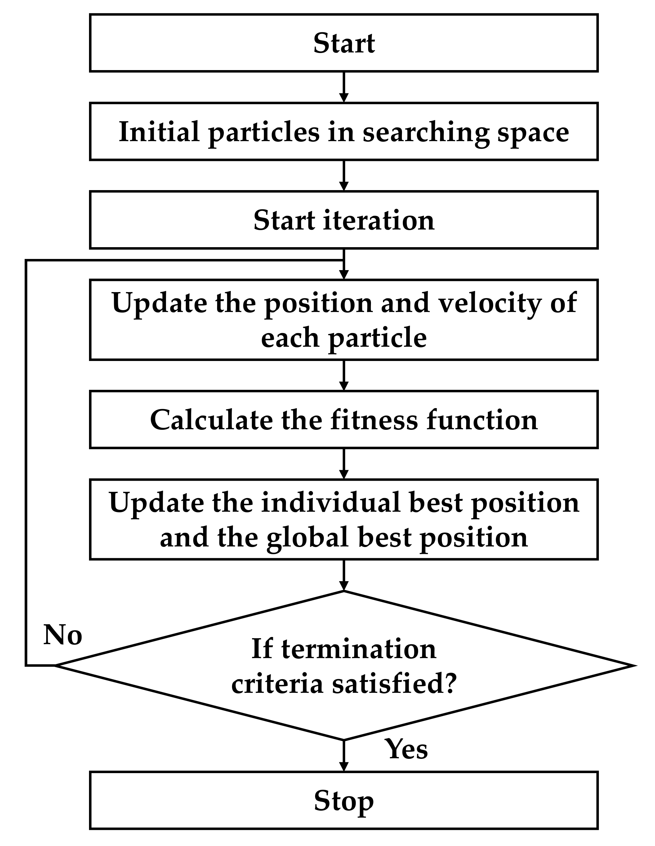
4. Experimental Results

In this section, the results of the experiment are discussed. The flowchart of the proposed online tuning method is shown in Figure 8. First, the approximate model of the motor was obtained by the system identification. To verify the stability of the system, the Routh–Hurwitz [49] stability criterion was used. Afterward, the searching regions of $K_p$ and $K_i$ could be determined. By using the Hall sensor and speed sensor, the current signal and the motor speed could be acquired. When a significant change happened in the motor speed, the tuning algorithm started. In this study, three tuning methods, including the fixed method, PSO algorithm, and DDPG, were compared. Finally, the desired parameters of $K_p$ and $K_i$ could be obtained and updated in the actuator.

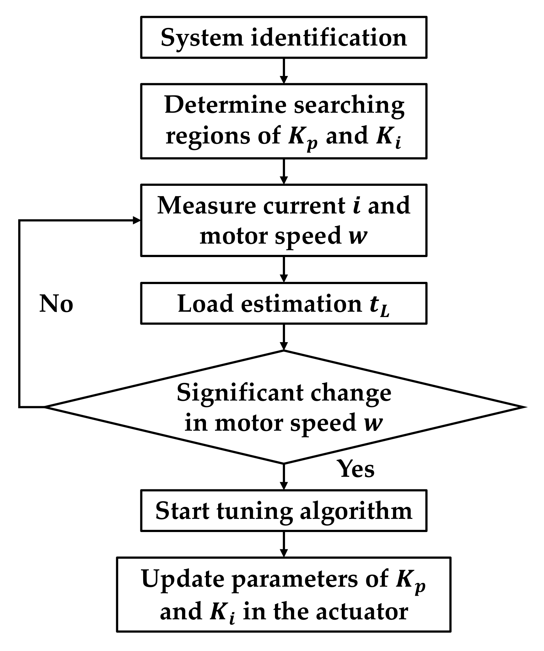
4.1. System Description and Stability

The motor system was considered to be a two-order transfer function, which is shown in Equation (1). By measuring the three-phase current and the output speed, and using the MATLAB system identification toolbox, the coefficients of $A$, $B$, $C$, and $D$ were found to be 4.4720${\times 10}^{-4}$, 1.0181, 3.9129, and 886.21519, respectively. To confirm the performance of the system identification process, motor under settings of $K_p=226$ and $K_i=36$ were tested. 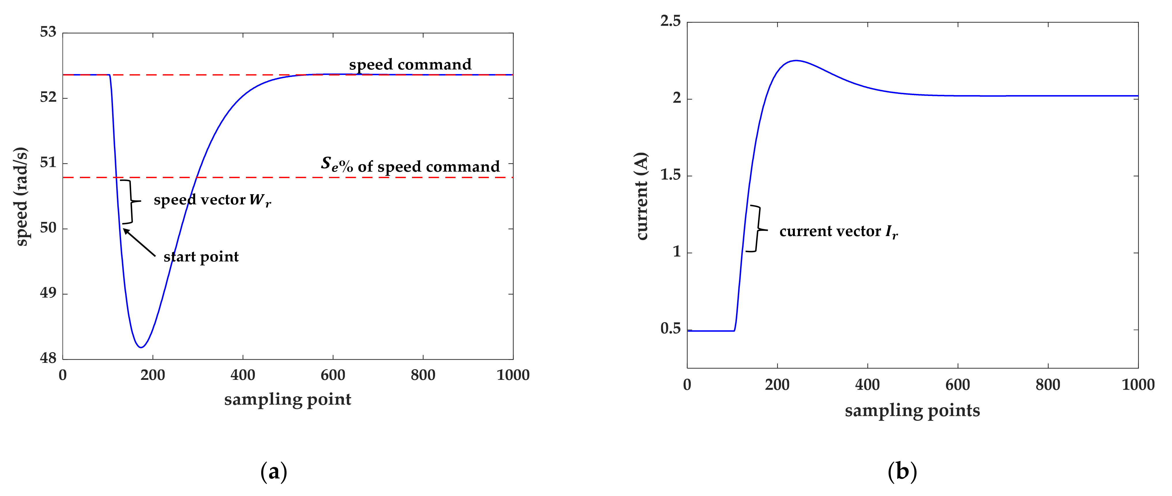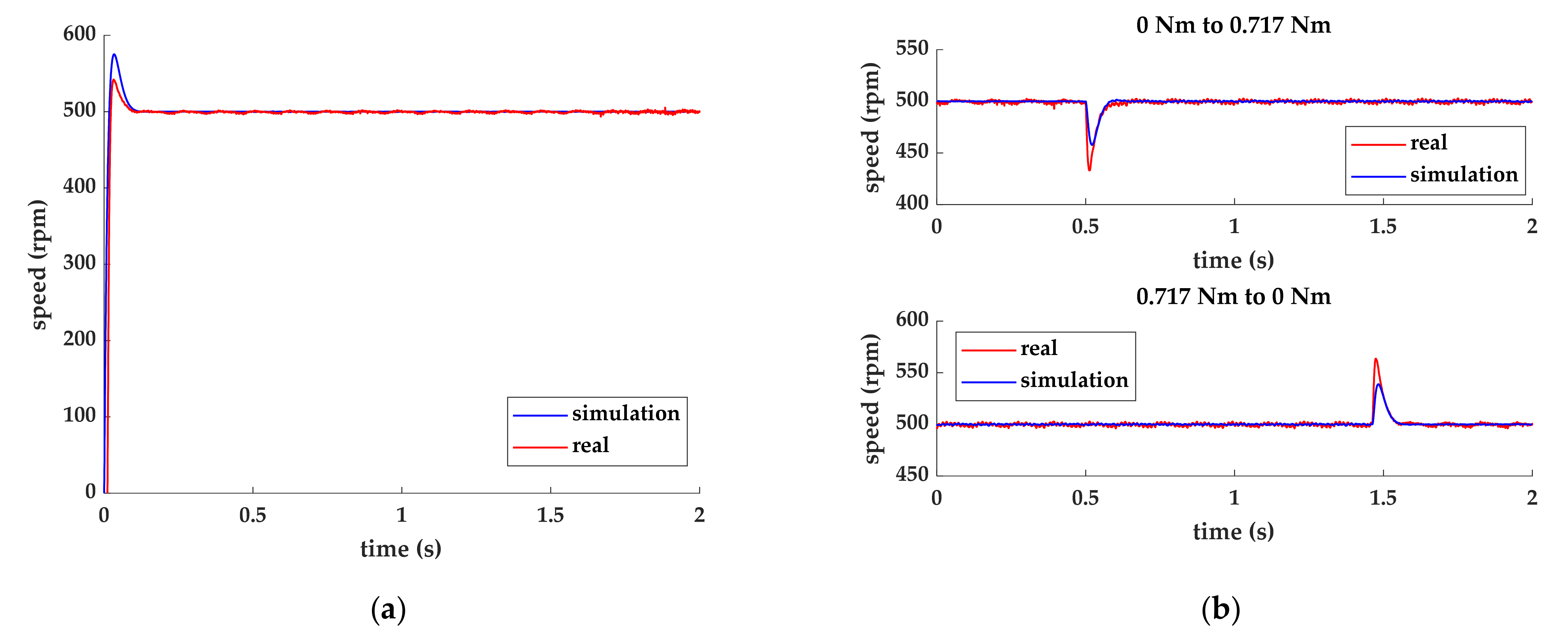Figure 9a illustrates the transient and steady state response under the command speed of 500 rpm. In addition, Figure 9b shows the speed response to load disturbance. The results show that the settling times of the approximate model and the real motor were similar. However, different amounts of overshoot and undershoot were found to exist. In Figure 9a, it can be seen that the overshoots of the simulation and real motor were 15.0% and 8.4%, respectively. In Figure 9b, when adding a load to the motor, the undershoot of the simulation and real motor were found to be 8.4% and 13.4%, respectively. However, when releasing the load, the overshoot of the simulation and real motor were observed to be 7.7% and 12.7%, respectively.

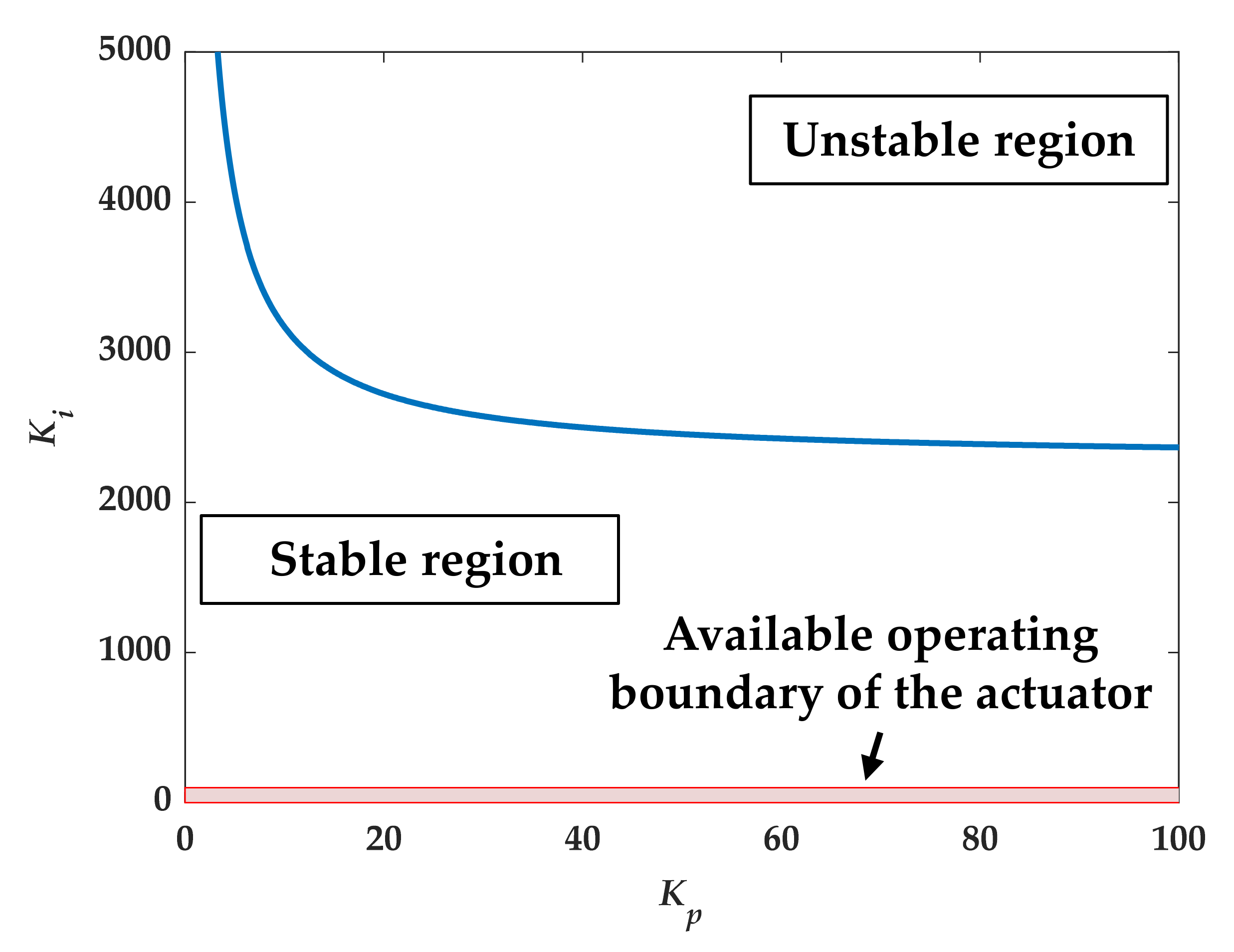
In order to implement the online learning method, the stability of the system needed to be considered. Inappropriate tuning parameters would cause the system to be unstable. According to the Routh–Hurwitz criterion, the stable boundaries of $K_p$ and $K_i$ that cause the system to be stable were calculated and are shown in Figure 10. The positive area below the blue curve is the stable region. As mentioned in Section 3.4.2, the available setting ranges of $K_p$ and $K_i$ of the actuator were [0, 500] and [0, 100], respectively. The available operating area, the red boundary, is shown in Figure 10. All the operating area was in the stable region. Hence, the settings of the actuator were all allowed.

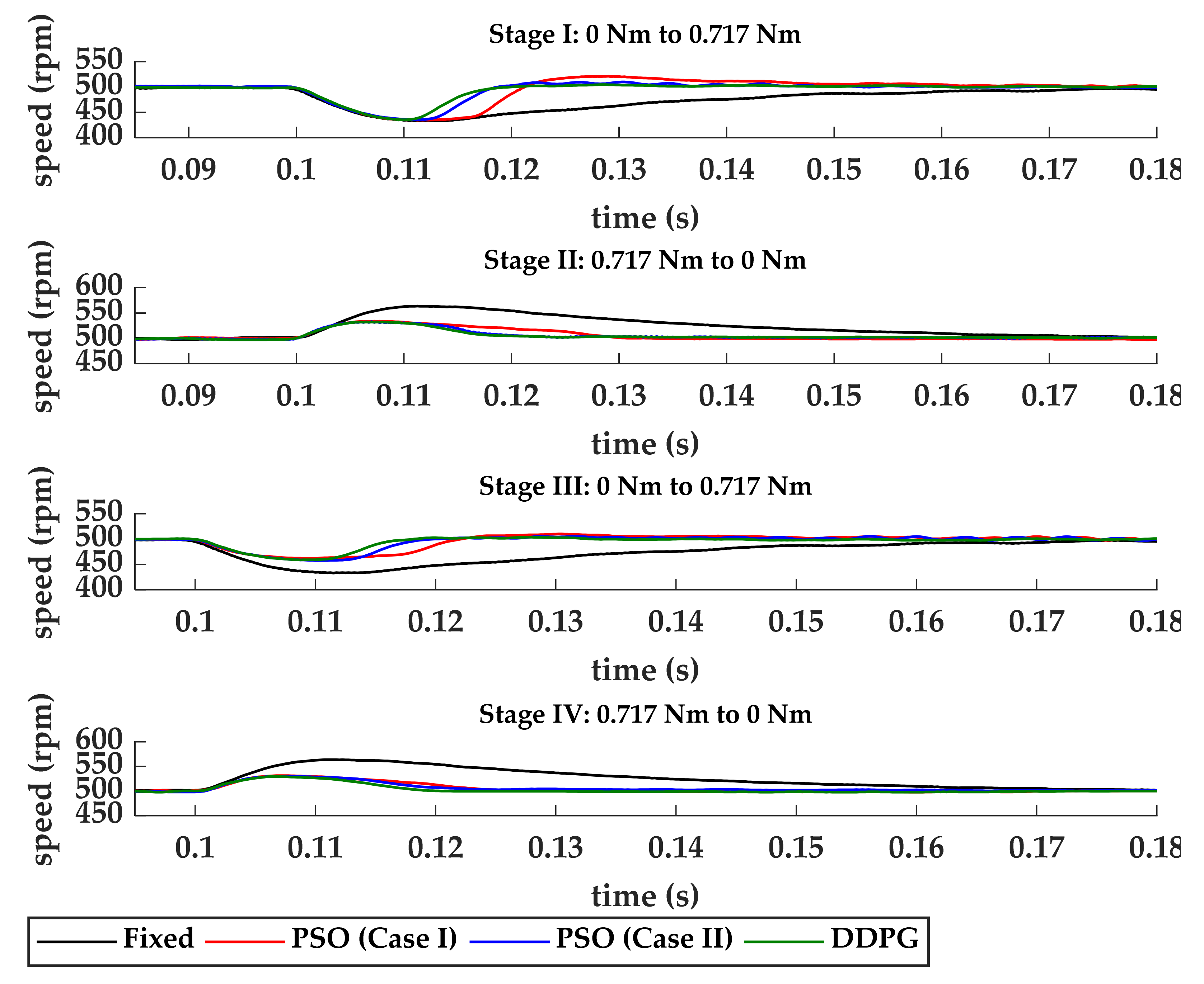
4.2. Online-Tuning Results

The experiment was divided into four stages representing the load conditions of 0$\to$0.717 Nm, 0.717$\to$0 Nm, 0$\to$0.717 Nm, and 0.717$\to$0 Nm, respectively. Figure 11 shows the comparison of the four methods. As shown in Figure 11, using fixed values of $K_p$ and $K_i$, the settling time, undershoot and overshoot were about 100 ms, 13.4%, and 12.7%, respectively. To improve the performance of the time response, PSO tuning method is first discussed. Two parameter settings of PSO algorithm are shown in

Table 5. Two parameter settings of PSO algorithm.

Case	Parameters
	Particle Number	Iteration Number	${\mathit{w}}_{\mathit{p}}$	${\mathit{C}}_1$	${\mathit{C}}_2$	${\mathit{S}}_{\mathit{e}}\%$	${\mathit{N}}_{\mathit{e}}$	Number of Predicted Points
I	25	10	0.5	1.2	1.2	97	20	300
II	25	5	0.5	1.2	1.2	98.5	10	300

.

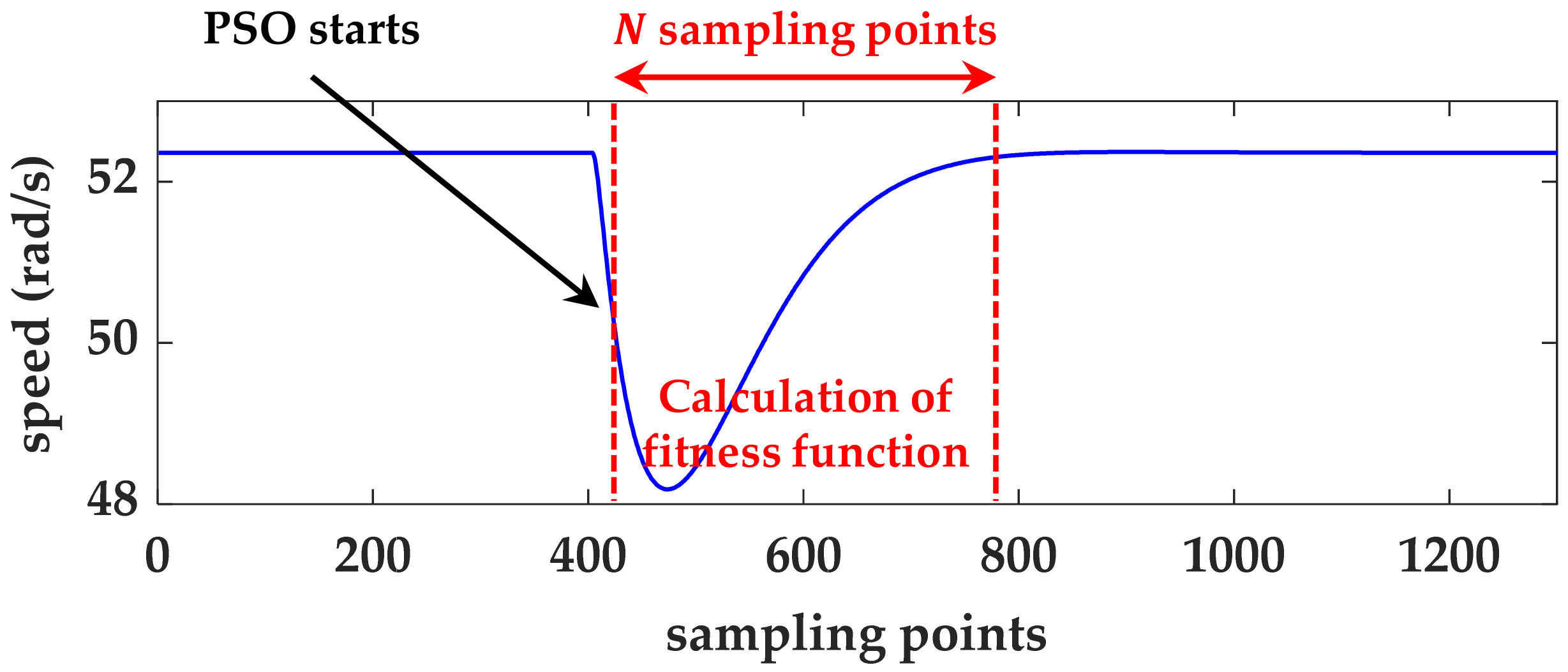
In Case I, when twenty continuous sampling points of the rotating speed was lower than 97% of the command speed, the PSO tuning method started. To calculate the fitness equation $T_{IAE}$ as shown in Equation (15), 300 sampling points of the speed response after the starting point were predicted by Equations (5) and (10). Subsequently, the sub-optimized solutions could be obtained and sent into the actuator.

First, for comparison with the fixed method, the values of $K_p$ and $K_i$ were initialized to 226 and 36. In stage I, the settling time could be improved from 100 ms to 58 ms. However, the undershoot did not undergo significant change, and was about 13%. In stage II, the settling time was decreased to 39 ms, which was 61 ms better than that of the fixed method. Moreover, the overshoot was decreased to 6.8%. To confirm the performance of the motor encountering the same load conditions, stages III and IV were conducted. In stage III, the settling time and undershoot were 34 ms and 7.6%, respectively. Because the values of $K_p$ and $K_i$ had been tuned, a better ability to compensate the current is shown. In stage IV, the settling time was 34 ms, and the overshoot was 6.26% which was 0.54% better than that in stage II. The results suggest that the performance of the time response was improved. However, the tuning results were affected by the computational consumption and delay time. In stage I, the real tuning point was operated after the lowest point, which was far from the start point. The delay time caused the solutions determined by the PSO algorithm to be sub-optimized solutions. In Case I, the PSO algorithm took about 2 ms to yield the solutions. In addition, the delay time of communicating with the actuator was about 10 ms. The results show that the time consumption is an important issue.

In order to minimize the influence of computational time and delay time, some parameter settings were changed. In Case II, the threshold $S_e$, error number $N_e$, and the iteration number were modified to 98.5% and 5. By changing the settings, the calculation time of the PSO algorithm was reduced to 1 ms. A lower value of $S_e$ led the tuning method to be more sensitive to the speed error; however, it made the start point move forward by about 2.5 ms.

In stage I, the settling time was about 28 ms, which was 22 ms better than that of Case I. However, the change of the settings did not make great improvement on the undershoot. In stage II, the settling time was decreased to 20 ms. Furthermore, the overshoot was decreased to 6.4%. In stage III, the settling time and undershoot were 19 ms and 8.3%, respectively. In stage IV, the settling time was 22 ms, and overshoot was 6.26%. The results show that, by reducing the processing time, some parts of the performance could be improved.

To deal with the delay time problem and imprecise mathematical model, DDPG model-free reinforcement learning was used to train online. By observing the experimental results of Cases I and II, the values of $S_e$ and $N_e$ were set to 98.5% and 10 in the Cases of DDPG. In addition, the TensorFlow Lite technique was utilized to accelerate the prediction process without losing accuracy. The prediction time could be reduced to 0.03 ms, which was about 300 times smaller than that of Case II. As illustrated in Figure 11, when a load was added to the motor, the DDPG method could provide the best current compensation. The settling times in stages I and II were 18 and 16 ms, which were the smallest values in each Case. When releasing the load, in stages II and IV, the settling times were 20 ms and 18 ms, respectively.

Table 6. Values of settling time, undershoot, and overshoot of each method.

Methods	Time Response
	Settling Time (ms)				Undershoot/Overshoot (%)
	Stage I	Stage II	Stage III	Stage IV	Stage I	Stage II	Stage III	Stage IV
Fixed	100	100	100	100	$\approx$13.4	12.7	13.4	12.7
PSO (Case I)	58	39	34	34	$\approx$13.4	6.8	7.6	6.3
PSO (Case II)	28	20	19	22	$\approx$13.4	6.4	8.3	6.3
DDPG	18	16	20	18	$\approx$13.4	6.5	8.0	6.3

list the values of settling time, undershoot, and overshoot of each method. The fixed value settings obtained from the Delta actuator performed the worst. For the undershoot and overshoot, the other three methods had similar performance. However, for the settling time, the proposed method had the smallest values.

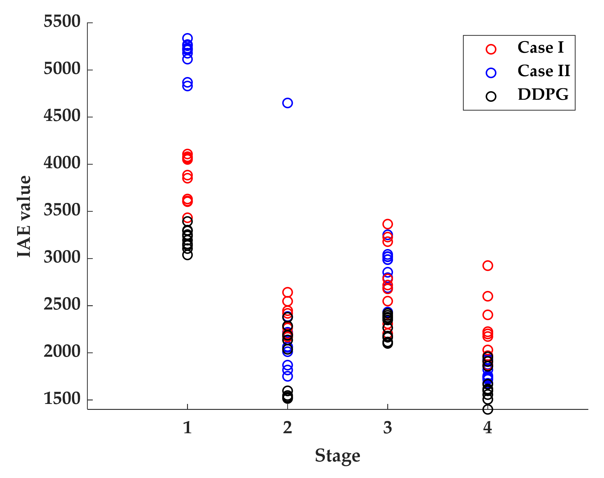
Figure 12 shows ten experimental results of the IAE calculation in different stages for each method. In Case I, the average IAE values of each stage were 5151.84, 2305.85, 2908.35, and 1792.76, respectively. In Case II, the average IAE values of each stage were 3831.83, 2333.24, 2718.14, and 2230.39, respectively. Generally, in stage I, the tuning results of Case II were better than those of Case I. Because the starting point was moved forward and the calculation time was decreased, the solutions of $K_p$ and $K_i$ could operate at a more suitable point. In stages II and III, the average IAE values were similar. In stage IV, the tuning results of Case I were better than those of Case II. Furthermore, in Case I, the standard deviations of each stage were 169.69, 205.41, 277.11, and 89.92, respectively. In Case II, the standard deviations of each stage were 246.02, 169.64, 429.51, and 322.51, respectively. The solutions of Case II were more separated, which was caused by the smaller number of iterations. However, some solutions determined by Case II were better than Case I.

The average IAE values of the proposed DDPG showed the best performance. Furthermore, according to the standard deviation of the IAE value, the solutions determined by the proposed DDPG were more converged, which is shown in Figure 12.

Table 7. IAE value of each Case.

Methods	IAE Value
	Average				Standard Deviation
	Stage I	Stage II	Stage III	Stage IV	Stage I	Stage II	Stage III	Stage IV
Fixed	8906.63	8674.13	8887.93	8641.33	50.31	105.52	19.74	70.90
PSO (Case I)	5151.84	2305.85	2908.35	1792.76	169.69	859.26	277.11	89.92
PSO (Case II)	3831.83	2333.24	2718.14	2230.39	246.02	169.64	429.51	322.51
DDPG	3279.09	1956.57	2303.54	1693.80	100.20	356.02	119.93	187.66

lists the average and standard deviation of the IAE value of the four methods. The experimental results show that the DDPG method combines the advantages of Cases I and II. The proposed method can learn the unknown model of the motor system and determine better tuning solutions for the load disturbance.

5. Conclusions

This study proposed a DDPG method to effectively track the speed control under an unknown load disturbance. A precise mathematical model of the motor system is not required when using the model-free reinforcement learning algorithm. Three methods, including the fixed method, PSO algorithm, and DDPG, were discussed. The fixed method showed the worst performance. The fixed values of $K_p$ and $K_i$, 226 and 36, were provided by the Delta actuator based on the motor status and settings. It took the longest time to return back to the speed command, and had the largest overshoot and undershoot. The tuning results of the PSO algorithm show that the speed response was improved when the load disturbance occurred. However, the computational time and time delay caused by communicating to the actuator affected the tuning performance. To solve the mentioned challenges, the DDPG method was proposed. The sub-optimized solutions of $K_p$ and $K_i$ determined by the PSO algorithm were added into the DDPG training, which caused the training to converge faster and more safely. Through the use of Tensorflow Lite, the computational time challenge could be solved. The experimental results show that the proposed DDPG method was able to effectively decrease the settling time, overshoot, and undershoot under the load disturbance. The proposed technique can be used in the field of machining. In the cutting process, the speed of the motor usually decreases when the external load suddenly becomes large. To obtain a smooth surface and high quality of the parts, the fast compensation method of the motor speed can be utilized.

References

1. Cruz, A.G.d.A.; Gomes, R.D.; Belo, F.A.; Lima-Filho, A. A Hybrid System Based on Fuzzy Logic to Failure Diagnosis in Induction Motors. IEEE Lat. Am. Trans. 2017, 15, 1480–1489. [Google Scholar] [CrossRef]
2. Sant, A.V.; Rajagopal, K.; Sheth, N.K. Permanent Magnet Synchronous Motor Drive Using Hybrid PI Speed Controller with Inherent and Noninherent Switching Functions. IEEE Trans. Magn. 2011, 47, 4088–4091. [Google Scholar] [CrossRef]
3. Gashtil, H.; Pickert, V.; Atkinson, D.; Giaouris, D.; Dahidah, M. Comparative evaluation of field oriented control and direct torque control methodologies in field weakening regions for interior permanent magnet machines. In Proceedings of the 2019 IEEE 13th International Conference on Compatibility, Power Electronics and Power Engineering, Sonderborg, Denmark, 23–25 April 2019. [Google Scholar]
4. Liu, Q.; Zha, Y.; Liu, T.; Lu, C. Research on adaptive control of airborne bolting rigs based on genetic algorithm optimization. Machines 2021, 9, 10. [Google Scholar] [CrossRef]
5. Hayashi, A.; Nakao, Y. Rotational speed control system of water driven spindle considering influence of cutting force using disturbance observer. Precis. Eng. 2018, 51, 88–96. [Google Scholar] [CrossRef]
6. Ciccarelli, D.; El Mehtedi, M.; Forcellese, A.; Greco, L.; Simoncini, M. In-process Control of Rotational Speed in Friction Stir Welding of Sheet Blanks with Variable Mechanical Properties. Procedia CIRP 2018, 67, 440–445. [Google Scholar] [CrossRef]
7. Huba, M.; Chamraz, S.; Bistak, P.; Vrancic, D. Making the PI and PID Controller Tuning Inspired by Ziegler and Nichols Precise and Reliable. Sensors 2021, 21, 6157. [Google Scholar] [CrossRef]
8. He, Z.; Nie, L.; Yin, Z.; Huang, S. A Two-Layer Controller for Lateral Path Tracking Control of Autonomous Vehicles. Sensors 2020, 20, 3689. [Google Scholar] [CrossRef]
9. Li, K.; Boonto, S.; Nuchkrua, T. On-line Self Tuning of Contouring Control for High Accuracy Robot Manipulators under Various Operations. Int. J. Control. Autom. Syst. 2020, 18, 1818–1828. [Google Scholar] [CrossRef]
10. Sant, A.V.; Rajagopal, K.R. PM Synchronous motor speed control using hybrid fuzzy-PI with novel switching functions. IEEE Trans. Magn. 2009, 45, 4672–4675. [Google Scholar] [CrossRef]
11. Aghili, F. Optimal feedback linearization control of interior PM synchronous motors subject to time-varying operation condi-tions minimizing power loss. IEEE Trans. Ind. Electron. 2018, 65, 5414–5421. [Google Scholar] [CrossRef]
12. Li, Z.; Zhou, S.; Xiao, Y.; Wang, L. Sensorless Vector Control of Permanent Magnet Synchronous Linear Motor Based on Self-Adaptive Super-Twisting Sliding Mode Controller. IEEE Access 2019, 7, 44998–45011. [Google Scholar] [CrossRef]
13. Mier, L.; Benitez, J.; Lopez, R.; Segovia, J.; Peña-Eguiluz, R.; Ramirez, F.J.J. Adaptive Fuzzy Control System for a Squirrel Cage Induction Motor. IEEE Lat. Am. Trans. 2017, 15, 795–805. [Google Scholar] [CrossRef]
14. Ahmed, A.A.; Koh, B.K.; Lee, Y.I. A comparison of Finite control set and continuous control set model predictive control schemes for speed control of induction motors. IEEE Trans. Ind. Inform. 2018, 14, 1334–1346. [Google Scholar] [CrossRef]
15. Bolognani, S.; Peretti, L.; Zigliotto, M. Design and Implementation of Model Predictive Control for Electrical Motor Drives. IEEE Trans. Ind. Electron. 2009, 56, 1925–1936. [Google Scholar] [CrossRef]
16. Kennedy, J.; Eberhart, R. Particle swarm optimization. In Proceedings of the ICNN’95—International Conference on Neural Networks, Perth, WA, Australia, 27 Noverber–1 December 1995; IEEE: Piscataway, NJ, USA; Volume 4, pp. 1942–1948. [Google Scholar]
17. Gharghan, S.K.; Nordin, R.; Ismail, M.; Ali, J.A. Accurate Wireless Sensor Localization Technique Based on Hybrid PSO-ANN Algorithm for Indoor and Outdoor Track Cycling. IEEE Sens. J. 2016, 16, 529–541. [Google Scholar] [CrossRef]
18. Ye, Y.; Yin, C.-B.; Gong, Y.; Zhou, J.-J. Position control of nonlinear hydraulic system using an improved PSO based PID controller. Mech. Syst. Signal Process. 2017, 83, 241–259. [Google Scholar] [CrossRef]
19. Lin, C.-J.; Li, T.-H.S.; Kuo, P.-H.; Wang, Y.-H. Integrated particle swarm optimization algorithm based obstacle avoidance control design for home service robot. Comput. Electr. Eng. 2016, 56, 748–762. [Google Scholar] [CrossRef]
20. Perng, J.-W.; Chen, G.-Y.; Hsieh, S.-C. Optimal PID Controller Design Based on PSO-RBFNN for Wind Turbine Systems. Energies 2014, 7, 191–209. [Google Scholar] [CrossRef] [Green Version]
21. Usama, M.; Qadir, J.; Raza, A.; Arif, H.; Yau, K.-L.A.; Elkhatib, Y.; Hussain, A.; Al-Fuqaha, A. Unsupervised Machine Learning for Networking: Techniques, Applications and Research Challenges. IEEE Access 2019, 7, 65579–65615. [Google Scholar] [CrossRef]
22. Sen, P.C.; Hajra, M.; Ghosh, M. Supervised Classification Algorithms in Machine Learning: A Survey and Review. In Emerging Technology in Modelling and Graphics; Springer: Singapore, 2020; pp. 99–111. [Google Scholar] [CrossRef]
23. Liu, C.; Xu, X.; Hu, D. Multiobjective Reinforcement Learning: A Comprehensive Overview. IEEE Trans. Syst. Man Cybern. Syst. 2015, 45, 385–398. [Google Scholar] [CrossRef]
24. Luwei, K.C.; Yunusa-Kaltungo, A.; Sha’aban, Y.A. Integrated fault detection framework for classifying rotating machine faults using frequency domain data fusion and artificial neural networks. Machines 2018, 6, 59. [Google Scholar] [CrossRef] [Green Version]
25. Seong, J.H.; Seo, D.H. Selective Unsupervised Learning-Based Wi-Fi Fingerprint System Using Autoencoder and GAN. IEEE Internet Things J. 2020, 7, 1898–1909. [Google Scholar] [CrossRef]
26. Van der Maaten, L.; Hinton, G. Visualizing high-dimensional data using t-SNE. J. Mach. Learn. Res. 2008, 9, 2579–2605. [Google Scholar]
27. Won, C.S. Multi-Scale CNN for Fine-Grained Image Recognition. IEEE Access 2020, 8, 116663–116674. [Google Scholar] [CrossRef]
28. Moreira, L.; Figueiredo, J.; Vilas-Boas, J.; Santos, C. Kinematics, Speed, and Anthropometry-Based Ankle Joint Torque Estimation: A Deep Learning Regression Approach. Machines 2021, 9, 154. [Google Scholar] [CrossRef]
29. Chiu, Y.-C.; Wang, P.-H.; Hu, Y.-C. The thermal error estimation of the machine tool spindle based on machine learning. Machines 2021, 9, 184. [Google Scholar] [CrossRef]
30. Wu, B.-F.; Lin, C.-H. Adaptive neural predictive control for permanent magnet synchronous motor systems with long delaytime. IEEE Access 2019, 7, 108061–108069. [Google Scholar] [CrossRef]
31. Watkins, C.J.C.H.; Dayan, P. Q-learning. Mach. Learn. 1992, 8, 279–292. [Google Scholar] [CrossRef]
32. Mnih, V.; Kavukcuoglu, K.; Silver, D.; Graves, A.; Antonoglou, I.; Wierstra, D.; Riedmiller, M. Playing Atari with deep reinforcement learning. arXiv 2013, arXiv:1312.5602. [Google Scholar]
33. Schenke, M.; Wallscheid, O. A Deep Q-Learning Direct Torque Controller for Permanent Magnet Synchronous Motors. IEEE Open J. Ind. Electron. Soc. 2021, 2, 388–400. [Google Scholar] [CrossRef]
34. Sutton, R.; McAllester, D.; Singh, S.; Mansour, Y. Policy gradient methods for reinforcement learning with function approximation. Adv. Neural Inf. Process. Syst. 2000, 12, 1057–1063. [Google Scholar]
35. Lillicrap, T.P. Continuous control with deep reinforcement learning. arXiv 2015, arXiv:1509.02971. [Google Scholar]
36. Fujimoto, S.; Hoof, H.; Meger, D. Addressing function approximation error in Actor-Critic methods. In Proceedings of the 35th International Conference on Machine Learning, Stockholm, Sweden, 10–15 July 2018. [Google Scholar]
37. Haarnoja, T. Soft Actor-Critic algorithms and applications. arXiv 2018, arXiv:1812.05905. [Google Scholar]
38. Liu, M.; Zhao, F.; Niu, J.; Liu, Y. ReinforcementDriving: Exploring Trajectories and Navigation for Autonomous Vehicles. IEEE Trans. Intell. Transp. Syst. 2021, 22, 808–820. [Google Scholar] [CrossRef]
39. Jin, L.; Tian, D.; Zhang, Q.; Wang, J. Optimal torque distribution control of multi-axle electric vehicles with in-wheel motors based on DDPG algorithm. Energies 2020, 13, 1331. [Google Scholar] [CrossRef] [Green Version]
40. Takasaki, G.; Fenton, R. On the identification of vehicle longitudinal dynamics. IEEE Trans. Autom. Control. 1977, 22, 610–615. [Google Scholar] [CrossRef]
41. Chen, G.Y.; Perng, J.-W. PI speed controller design based on GA with time delay for BLDC motor using DSP. In Proceedings of the 2017 IEEE International Conference on Mechatronics and Automation (ICMA), Takamatsu, Japan, 24 August 2017; IEEE: Piscataway, NJ, USA, 2017; pp. 1174–1179. [Google Scholar]
42. Bicakci, S. On the Implementation of Fuzzy VMC for an Under Actuated System. IEEE Access 2019, 7, 163578–163588. [Google Scholar] [CrossRef]
43. Rahimi, T.; Ding, L.; Kheshti, M.; Faraji, R.; Guerrero, J.M.; Tinajero, G.D.A. Inertia response coordination strategy of wind generators and hybrid energy storage and operation cost-based multi-objective optimizing of frequency control parameters. IEEE Access 2021, 9, 74684–74702. [Google Scholar] [CrossRef]
44. Yousaf, S.; Mughees, A.; Khan, M.G.; Amin, A.A.; Adnan, M. A Comparative Analysis of Various Controller Techniques for Optimal Control of Smart Nano-Grid Using GA and PSO Algorithms. IEEE Access 2020, 8, 205696–205711. [Google Scholar] [CrossRef]
45. Wasala, A.; Byrne, D.; Miesbauer, P.; O’Hanlon, J.; Heraty, P.; Barry, P. Trajectory based lateral control: A Reinforcement Learning case study. Eng. Appl. Artif. Intell. 2020, 94, 103799. [Google Scholar] [CrossRef]
46. Lin, G.; Zhu, L.; Li, J.; Zou, X.; Tang, Y. Collision-free path planning for a guava-harvesting robot based on recurrent deep reinforcement learning. Comput. Electron. Agric. 2021, 188, 106350. [Google Scholar] [CrossRef]
47. Zou, Y.; Chen, T.; Chen, X.; Li, J. Robotic seam tracking system combining convolution filter and deep reinforcement learning. Mech. Syst. Signal Process. 2022, 165, 108372. [Google Scholar] [CrossRef]
48. Yu, W.; Lv, P. An End-to-End Intelligent Fault Diagnosis Application for Rolling Bearing Based on MobileNet. IEEE Access 2021, 9, 41925–41933. [Google Scholar] [CrossRef]
49. Khatwani, K. On Routh-Hurwitz criterion. IEEE Trans. Autom. Control. 1981, 26, 583–584. [Google Scholar] [CrossRef]
Figure 1. Motor testing platform: (1) motor I; (2) speed sensor; and (3) motor II.
Machines 09 00343 g001
Figure 2. Peripheral devices: (1) power supplier; (2) signal amplifier of speed sensor; (3) USB-2405; (4) hall sensor; (5) actuator; and (6) regenerative resistor.
Machines 09 00343 g002
Figure 4. Operation of the PSO algorithm.
Machines 09 00343 g004
Figure 5. Flowchart of the PSO algorithm.
Machines 09 00343 g005
Figure 6. Signals fed into the actor network under the conditions of speed command 52.359 rad/s and load disturbance 0.717 Nm: (a) speed and (b) current.
Machines 09 00343 g006
Figure 7. Architectures of the networks: (a) actor and (b) critic.
Machines 09 00343 g007
Figure 8. Flowchart of the proposed online-tuning method.
Machines 09 00343 g008
Figure 9. Motor speed response: (a) transient and steady state response, and (b) speed response with disturbance load of 0.717 Nm.
Machines 09 00343 g009
Figure 10. Stable range of K p and K i for the system.
Machines 09 00343 g010
Figure 11. Comparison of the four tuning methods.
Machines 09 00343 g011
Figure 12. IAE values in each stage.
Machines 09 00343 g012