Article

Forward and Inverse Dynamics of a Unicycle-Like Mobile Robot

by
Carmine Maria Pappalardo
* and
Domenico Guida
Department of Industrial Engineering, University of Salerno, Via Giovanni Paolo II 132, 84084 Fisciano, Italy
*
Author to whom correspondence should be addressed.
Machines 2019, 7(1), 5; https://doi.org/10.3390/machines7010005
Submission received: 6 November 2018 / Revised: 3 January 2019 / Accepted: 8 January 2019 / Published: 11 January 2019

Abstract

:
In this research work, a new method for solving forward and inverse dynamic problems of mechanical systems having an underactuated structure and subjected to holonomic and/or nonholonomic constraints is developed. The method devised in this paper is based on the combination of the Udwadia-Kalaba Equations with the Underactuation Equivalence Principle. First, an analytical method based on the Udwadia-Kalaba Equations is employed in the paper for handling dynamic and control problems of nonlinear nonholonomic mechanical systems in the same computational framework. Subsequently, the Underactuation Equivalence Principle is used for extending the capabilities of the Udwadia-Kalaba Equations from fully actuated mechanical systems to underactuated mechanical systems. The Underactuation Equivalence Principle represents an efficient method recently developed in the field of classical mechanics. The Underactuation Equivalence Principle is used in this paper for mathematically formalizing the underactuation property of a mechanical system considering a particular set of nonholonomic algebraic constraints defined at the acceleration level. On the other hand, in this study, the Udwadia-Kalaba Equations are analytically reformulated in a mathematical form suitable for treating inverse dynamic problems. By doing so, the Udwadia-Kalaba Equations are employed in conjunction with the Underactuation Equivalence Principle for developing a nonlinear control method based on an inverse dynamic approach. As shown in detail in this investigation, the proposed method can be used for analytically solving in an explicit manner the forward and inverse dynamic problems of several nonholonomic mechanical systems. In particular, the tracking control of the unicycle-like mobile robot is considered in this investigation as a benchmark example. Numerical experiments on the dynamic model of the unicycle-like mobile robot confirm the effectiveness of the nonlinear dynamic and control approaches developed in this work.

1. Introduction

In this section, background information is provided first. Subsequently, the problem of interest for this investigation is formulated and a brief literature survey is reported. Then, the scope and the contributions of this paper are described and the organization of the manuscript is summarized.

1.1. Background

In industrial applications, the final design solution of a new product is almost always an engineering approximation that is intrinsically prone to unpredictable uncertainties [1,2,3,4,5,6,7]. A viable approach to the analysis of the approximation in a given design solution is based on the use of a reasonably complex mathematical model of the mechanical system at hand [8,9,10,11]. A mathematical model covers almost all physical, economical, biological, industrial, and technical phenomena [12,13,14,15,16,17,18]. In particular, dynamic models can be used for the development of new control algorithms suitable for solving several engineering problems [19,20,21,22,23,24]. This process is particularly effective in the field of robotics for controlling mobile robots that represent the main object of the present research work [25,26,27,28,29,30].

1.2. Formulation of the Problem of Interest for This Study

In the last thirty years, the use of mobile robots has gained great attention because of their broad potential in practical applications oriented toward the solution of important engineering problems [31,32,33,34,35,36]. For this purpose, several control approaches were developed for obtaining the stabilization and the trajectory tracking control of mobile robots [37,38,39,40,41,42,43]. In particular, in the field of robotics, the advantage of using wheeled mobile robots instead of legged mobile robots is widely accepted. When compared with legged mobile robots, wheeled mobile robots have a simple mechanical structure and, consequently, a mathematical model of this class of robots can be easily obtained. Legged mobile robots, on the other hand, are more versatile machines which make use of mechanical limbs for their movement and, therefore, can easily traverse several different terrains. The advantages in terms of dexterity of legged mobile robots over wheeled mobile robots involve a more complex structural design, a different paradigm for the construction of the robot, an increased power consumption, and require the development of a more complex control system. However, in general, both wheeled and legged mobile robots are subject to some degree of complexity in their mechanical behavior and, more importantly, their motion must satisfy some geometric constraints in order to be suitable for widely exploring the external environment [44,45,46,47,48]. One of the fundamental challenges associated with dynamic and control problems of both wheeled and legged mobile robots arise from the mathematical representation of their mechanical models which can be classified as underactuated nonholonomic dynamical systems. Underactuated mechanical systems are dynamical systems in which the number of control actuators is lower than the number of degrees of freedom. Moreover, nonholonomic dynamical systems are mechanical systems in which the constraint equations are of holonomic as well as nonholonomic nature, namely, they involve the complete set of generalized coordinates and their first and second time derivatives [49,50,51,52]. Thus, underactuated nonholonomic nonlinear mechanical systems represent a broad class of dynamical systems that are particularly challenging to analyze and control.

1.3. Literature Review

In the field of robotics, stabilization and tracking problems of mobile robots have grown in importance in recent years, as testified by a large number of research projects devoted to the investigation of these topics [53,54,55]. Furthermore, the nonlinear control problem focused on mobile robots have recently attracted significant attention in the control community because of the wide scope of applications of these mechanical systems [56,57,58,59,60,61,62,63]. In several engineering applications, mobile robots are often treated as mechanical systems constrained by holonomic and/or nonholonomic algebraic equations, which can be modeled employing nonlinear dynamics techniques such as the multibody approach to the dynamics of mechanical systems. In particular, wheeled mobile robots, which represent the mobile robots of interest for this investigation, must be modeled as nonholonomic mechanical systems to capture the pure rolling conditions of the wheels. Thus, the nonlinear control problem of this family of mechanical systems represents a challenging engineering issue [64,65,66,67]. In the literature, the nonlinear control methods employed for this class of mechanical systems are based on non-standard approaches that cannot be easily extended to both holonomic and nonholonomic mechanical systems [68,69,70]. For example, neural networks have been effectively used in recent years to approximate the dynamic behavior of mobile robots and for developing advanced nonlinear control strategies [71,72]. The control algorithms obtained by integrating kinematic controllers and neural network computed-torque controllers can be used for the solution of the three basic navigation problems associated with nonholonomic mobile robots, namely the tracking of a reference trajectory, the following of a prescribed path, and the stabilization around the desired configuration [73,74].
In this investigation, an effective control approach based on an inverse dynamic paradigm suitable for handling underactuated mechanical systems constrained by holonomic and/or nonholonomic algebraic equations is developed and its use is demonstrated by means of numerical experiments. The mobile robot that represents the object of this work is a wheeled robot having a unicycle-like underactuated structure. As described in detail in the paper, a unicycle-like mobile robot is a wheeled robot having three degrees of freedom that is endowed with a single steering wheel. This is a common design and is of great interest to engineers. The name unicycle for this type of mobile robot is commonly used also to remark the difference between this mobile robot and the bicycle mobile robot [75,76]. As mentioned before, the unicycle mobile robot has three degrees of freedom, is controlled by two control actuators, and is subjected to only one nonholonomic constraint equation associated with the pure rolling condition of the single wheel. The bicycle mobile robot, on the other hand, is endowed with four degrees of freedom, is controlled by using two control actuators, and is subjected to two nonholonomic constraint equations associated with the pure rolling conditions of the two wheels. Typically, the dynamic behavior of unicycle mobile robots is studied for testing nonlinear control strategies which can be directly extended to bicycle mobile robots. The performance of these control algorithms applied to bicycle mobile robots is particularly important because these mobile robots are kinematically equivalent to car-like mobile robots which are mechanically balanced. In the literature, the simple kinematic model this mobile robot is often used for investigating the performance of advanced control algorithms aimed at solving the stabilization, tracking, flocking, and rendezvous problems [77,78,79,80,81].

1.4. Scope and Contributions of This Research Work

This research work is focused on the dynamics and control of a unicycle-like mobile robot. The forward and inverse dynamic problems associated with the wheeled mobile robot considered in the paper represent archetypical examples pertaining to the general dynamic and control analysis of underactuated nonholonomic mechanical systems. To address these problems, the computational procedure developed in this investigation is based on an effective combination of the Udwadia-Kalaba Equations with the Underactuation Equivalence Principle. The Udwadia-Kalaba Equations allows for obtaining a clear and concise analytical formulation of dynamic problems which involve holonomic and/or nonholonomic algebraic constraints. Furthermore, as shown in this investigation, a general inverse dynamic method suitable for controlling nonlinear mechanical systems based on the Udwadia-Kalaba Equations can be readily devised and implemented. On the other hand, the Underactuation Equivalence Principle is a method recently developed in the field of analytical dynamics which allows for extending the application of the Udwadia-Kalaba Equations from fully actuated mechanical systems to underactuated mechanical systems. Therefore, as illustrated in this paper by means of detailed analytical derivations and extensive numerical computations, the Udwadia-Kalaba Equations can be effectively employed for solving forward and inverse dynamic problems associated with wheeled mobile robots. The Underactuation Equivalence Principle, on the other hand, is suitable for modeling underactuated nonholonomic mechanical systems and can be used for the synthesis of effective nonlinear control strategies. A unicycle-like mobile robot having one steerable drive wheel that is assumed to be always perpendicular to the ground, which represents one of the most common types of mobile robots employed in engineering applications, is used in this work for demonstrating the effectiveness of the inverse dynamic method devised in this investigation [82,83,84,85].

1.5. Organization of the Manuscript

This manuscript is organized as follows. In Section 2, the mathematical background related to Udwadia-Kalaba Equations and to the Underactuation Equivalence Principle is described in detail. In Section 3, the wheeled mobile robot having a unicycle-like underactuated structure used in the paper as a benchmark problem is illustrated and the derivation of a nonlinear tracking controller associated with a planar path described in a parametric form specifically designed for this mobile robot is analyzed. In Section 4, a discussion on the numerical results found by using the approach developed in the paper is reported and the directions for future research works are formulated. In Section 5, the summary of the paper and the conclusions obtained in this investigation are provided.

2. Background Material and Analytical Methods

In this section, the background material and the analytical methods of interest for this investigation are provided. First, the general form of the fundamental problem of constrained motion is recalled and, subsequently, these equations are rewritten in an analytical form suitable for solving inverse dynamics problems. Thereafter, the Udwadia-Kalaba Equations are discussed, and the Underactuation Equivalence Principle is presented. Moreover, the combined use of the Udwadia-Kalaba Equations with the Underactuation Equivalence Principle necessary for the development of nonlinear control laws suitable for controlling underactuated nonholonomic mechanical systems is analyzed.

2.1. Fundamental Problem of Constrained Dynamics

In this subsection, the general form of the fundamental problem of constrained motion is briefly recalled. In the central problem of constrained dynamics, the main goal is to predict the dynamical evolution of a mechanical system subjected to a given set of algebraic constraint equations [86,87,88]. For this purpose, the system initial conditions, namely the initial generalized coordinates and velocities, are specified data for the problem at hand. The external active forces not related to the kinematic constraints that are applied to the mechanical system are also assumed as known functions of time [89,90]. On the other hand, while the algebraic constraint equations represent specified limitations of the motion of the mechanical system and appear explicitly in the fundamental problem of constrained dynamics, the generalized constraint forces corresponding to the algebraic equations are additional unknowns of the dynamic problem to be solved [91,92].
An effective method for computing a closed-form analytical solution of the fundamental problem of constrained motion is based on the approach originally proposed by Udwadia and Kalaba [93]. The analytical method named after Udwadia and Kalaba is described in detail in a series of papers and in a book developed by the same authors [94,95]. For the purposes of the present study, the formulation and the solution of the general form of the fundamental problem of constrained motion developed by Udwadia and Kalaba can be summarized in the following steps. First, the equations of motion of a nonlinear mechanical system subjected to a general set of holonomic and/or nonholonomic constraints are analytically formulated by using the classical principles of analytical mechanics. Subsequently, the index-three form of the equations of motion is transformed into its index-one counterpart employing a standard index reduction technique. Finally, the general formulation of the Udwadia-Kalaba Equations is applied to the index-one form of the differential algebraic dynamic equations to obtain the system generalized acceleration vector and the generalized force vector associated with the algebraic constraints. In particular, an equivalent alternative form of the Udwadia-Kalaba Equations that is more suitable for describing the dynamic behavior of mechanical systems subjected to nonlinear algebraic constraints, such as multibody mechanical systems and wheeled mobile robots, is used in this paper.
The first step for the formulation and the solution of the fundamental problem of constrained dynamics is the analytical derivation of the equations of motion of a general mechanical system constrained by holonomic and/or nonholonomic constraints. To this end, the classical principles of analytical mechanics, such as the D’Alembert-Lagrange principle of virtual work formulated in conjunction with the Lagrange multiplier technique or the Lagrange equations, can be effectively used. To illustrate this fact, consider a nonlinear mechanical system described by a set of n b generalized coordinates that are used to represent the configuration space of the dynamical system [96]. Assume that the nonlinear mechanical system is initially unconstrained, namely the number of generalized coordinates n b of the dynamical system is equal to the number of the system degrees of freedom m f . In this case, it is well known that the equations of motion of a general unconstrained mechanical system can be directly obtained by using the Lagrange equations of the second kind. Thus, one can write:
d d t L q ˙ T L q T = Q e , n c
where t is time, q q ( t ) R n b denotes the generalized coordinate vector of the unconstrained mechanical system having dimension n b = m f , L L ( q , q ˙ , t ) identifies the Lagrangian function associated with the dynamical structure of the mechanical system, and Q e , n c Q e , n c ( q , q ˙ , t ) R n b represents the generalized force vector associated with the nonconservative external forces acting on the mechanical system. The generalized force vector associated with the nonconservative external forces Q e , n c can be found by calculating the virtual work of the nonconservative external forces as follows:
δ W e , n c = Q e , n c T δ q
where δ W e , n c δ W e , n c ( q , q ˙ , δ q ) denotes the virtual work of the nonconservative external forces applied on the mechanical system. For a given instant of time t, the generalized coordinate vector q and the generalized velocity vector q ˙ serve to determine uniquely the positions and the velocities of all the material points and rigid bodies that form the mechanical system [97]. Moreover, one can readily express the Lagrangian function of a mechanical systems as follows:
L = T U
where T T ( q , q ˙ , t ) identifies the kinetic energy associated with the inertial effects of the mechanical system and U U ( q , t ) denotes the potential energy relative to the conservative external forces acting on the dynamical system. For a mechanical system composed of rigid bodies, one can write the total kinetic energy of the nonlinear dynamical system in the following general form:
T = 1 2 q ˙ T M q ˙
where M M ( q , t ) R n b × n b is a positive-definite symmetric matrix that represents the system mass matrix. Considering the definition of the kinetic energy T given by Equation (4) as well as the general structure of the potential energy U, the application of the Lagrange equations of the second kind (1) leads to:
M q ¨ = T q T M ˙ q ˙ U q T + Q e , n c
or equivalently:
M q ¨ = Q v + Q e , c + Q e , n c
where Q v Q v ( q , q ˙ , t ) R n b is the inertia quadratic velocity vector which absorbs the generalized inertia effects associated with the squares of the generalized velocities and Q e , c Q e , c ( q , t ) R n b is the generalized force vector relative to the conservative external forces [98]. The inertia quadratic velocity vector Q v and the generalized force vector associated with the conservative external forces Q e , c are respectively given by:
Q v = T q T M ˙ q ˙ , Q e , c = U q T
It is, therefore, apparent that the definition of the Lagrangian function L of a nonlinear mechanical system and the specification of the virtual work associated with the nonconservative external forces δ W e , n c allow for calculating the equations of motion of a nonlinear mechanical system by using the Lagrange equations of the second kind given by Equation (1). For simplicity, one can rewrite the general form of the equations of motion of an unconstrained mechanical system given by Equation (6) as follows:
M q ¨ = Q b
where Q b Q b ( q , q ˙ , t ) R n b represents the total generalized force vector of the body forces relative to the mechanical system given by:
Q b = Q v + Q e , c + Q e , n c = Q v + Q e
where:
Q e = Q e , c + Q e , n c
where Q e Q e ( q , q ˙ , t ) R n b identifies the total generalized force vector associated with the external active forces. The equations of motion of a mechanical system written in the form given by Equation (8) constitute a nonlinear set of Ordinary Differential Equations (ODEs) in which the effect of the kinematic constraints is intrinsically embedded. This analytical description of the motion of a mechanical system is referred to as Minimal Coordinate Formulation (MCF) since by using this approach the general configuration of the mechanical system is represented employing a minimal set of generalized coordinates q formed by a vector of n b = m f variables [99]. In particular, the analytical approach based on the MCF leads to a set of equations of motion given by Equation (8) in which the generalized force vector associated with the algebraic constraints does not appear explicitly in accordance also with the basic assumption of ideal kinematic constraints or workless constraint forces. On the other hand, in principle, the same mechanical system can be equally described by using a Redundant Coordinate Formulation (RCF) in which an analytical approach based on a redundant set of generalized coordinates q is employed in order to univocally describe the geometric configuration of the mechanical system under consideration. In this case, the dimension of the generalized coordinate vector n b is larger than the number of the system degrees of freedom m f . In the RCF, the equations of motion can be readily obtained considering the Lagrange equations of the first kind as follows:
d d t L q ˙ T L q T = Q e , n c + Q c
where q identifies the redundant set of generalized coordinates having dimension n b > m f , L L ( q , q ˙ , t ) denotes the Lagrangian function associated with the redundant set of generalized coordinates, Q e , n c Q e , n c ( q , q ˙ , t ) R n b is the generalized force vector of the nonconservative external forces, and Q c Q c ( q , q ˙ , t ) R n b represents the total generalized force vector associated with the algebraic constraints applied to the mechanical system. Following the same mathematical manipulation previously used for the Lagrange equations of the second kind, the equations of motion of a general mechanical system expressed employing the analytical approach based on the RCF can be written as:
M q ¨ = Q b + Q c
where M M ( q , t ) R n b × n b denotes the system mass matrix associated with the redundant generalized coordinate vector and Q b Q b ( q , q ˙ , t ) R n b is the total generalized force vector of the body forces described by using the redundant coordinate approach. In the fundamental problem of constrained motion, the generalized force vector associated with the kinematic constraints Q c represents a set of additional unknowns of the problem. However, one can effectively use the Lagrange multiplier technique to express the analytical form of the generalized constraint force vector in terms of the vector of the Lagrange multipliers [100]. To this end, the algebraic equations that model the kinematic constraints can be effectively used.

2.2. Udwadia-Kalaba Equations in Forward and Inverse Dynamic Problems

In this subsection, the use of the Udwadia-Kalaba Equations for solving dynamic and control problems of nonlinear mechanical systems constrained by a general set of algebraic equations is discussed [101,102,103]. To this end, consider the following general form of the differential algebraic equations of motion of a mechanical system represented by using a redundant set of n b generalized coordinates whose motion is restricted by a set of n c algebraic constraints:
M q ¨ = Q b A T λ A q ¨ = b
where t is the time variable, q q ( t ) R n b is the generalized coordinate vector that represents that configuration of the mechanical system, q ˙ q ˙ ( t ) R n b represents the system generalized velocity vector, q ¨ q ¨ ( t ) R n b identifies the system generalized acceleration vector, M M ( q , t ) R n b × n b denotes the system mass matrix, Q b Q b ( q , q ˙ , t ) R n b identifies the total generalized force vector that acts on the mechanical system which includes the generalized external forces and the quadratic velocity inertial forces, λ λ ( t ) R n c represents the total vector of Lagrange multipliers associated with the constraint equations, A A ( q , t ) R n c × n b is the total Jacobian matrix relative to the constraint equations, and b b ( q , q ˙ , t ) R n c is the total constraint quadratic velocity vector. The index-three differential algebraic form of the dynamic equations is a general mathematical representation of the equations of motion of a nonlinear mechanical system that includes the effect of holonomic as well as nonholonomic constraints. In fact, considering a set of n f holonomic constraints defined at the position level, a set of n g nonholonomic constraints defined at the velocity level, and a set of n h nonholonomic constraints defined at the acceleration level, one can write the following general form of the algebraic equations:
f = 0 g = 0 h = 0
where f f ( q , t ) R n f is a nonlinear vector function associated with the holonomic constraint equations defined at the position level, g g ( q , q ˙ , t ) R n g denotes a nonlinear vector function relative to the nonholonomic constraint equations defined at the velocity level, and h h ( q , q ˙ , q ¨ , t ) R n h identifies a nonlinear vector function corresponding to the nonholonomic constraint equations defined at the acceleration level. This general set of constraint equations is included in the general form of the equations of motion by means of the total constraint Jacobian matrix denoted with A as well as considering the total constraint quadratic velocity vector indicated with b , which can be respectively obtained as follows:
A = A f A g A h , b = b f b g b h
where the total number of algebraic constraints is given by n c = n f + n g + n h , whereas A f A f ( q , t ) R n f × n b , A g A g ( q , t ) R n g × n b , and A h A h ( q , t ) R n h × n b respectively represent the Jacobian matrices relative to the algebraic constraint equations f , g , and h , while b f b f ( q , q ˙ , t ) R n f , b g b g ( q , q ˙ , t ) R n g , and b h b h ( q , q ˙ , t ) R n h respectively represent the quadratic velocity vectors associated with the algebraic constraint equations f , g , and h . These matrix and vector quantities are respectively defined as follows:
A f = f q A g = g q ˙ A h = h q ¨ , b f = f q q ˙ q q ˙ 2 f q t q ˙ f t t b g = g q q ˙ g t b h = c
where, for simplicity, the following structure of nonholonomic constraint equations defined at the acceleration level is assumed:
f q q ¨ + f q q ˙ q q ˙ + 2 f q t q ˙ + f t t = 0 g q ˙ q ¨ + g q q ˙ + g t = 0 h q ¨ q ¨ + c = 0
where the partial derivatives and the Jacobian matrices that appear in these equations are respectively defined as:
f q = f q , f q q ˙ q = f q q ˙ q , f q t = 2 f q t , f t t = 2 f t 2 g q ˙ = g q ˙ , g q = g q , g t = g t h q ¨ = h q ¨
where the term c c ( q , q ˙ , t ) R n h is assumed as a known nonlinear vector function. On the other hand, the Udwadia-Kalaba Equations can be written in a general form suitable for handling dynamic problems of nonlinear mechanical systems constrained by a general set of holonomic as well as nonholonomic constraints [104]. For this purpose, one can write:
q ¨ = a b + a c λ = Fe
where a b a b ( q , q ˙ , t ) R n b is the generalized acceleration vector of the mechanical system released from the constraint equations, a c a c ( q , q ˙ , t ) R n b is the generalized acceleration vector of the mechanical system induced by the constraint equations, F F ( q , q ˙ , t ) R n c × n c represents the constraint feedback matrix, and e e ( q , q ˙ , t ) R n c is the error vector associated with the generalized accelerations. The unconstrained acceleration vector a b can be explicitly computed by ignoring the action of the generalized constraint forces as follows:
a b = M 1 Q b
Furthermore, the acceleration error vector e can be analytically obtained by substituting the generalized acceleration vector corresponding to the unconstrained mechanical system a b into the set of constraint equations written in the standard form defined at the acceleration level:
e = b A a b
The constraint feedback matrix F , on the other hand, can be obtained by computing the Moore-Penrose pseudoinverse matrix of a special matrix associated with the constrained mechanical system. To this end, one can write:
F = K +
where the + symbol in the superscript indicates the Moore-Penrose pseudoinverse matrix and K K ( q , q ˙ , t ) R n c × n c is called the kinetic matrix of the constrained mechanical system. The kinetic matrix K is defined as follows:
K = A M 1 A T
The kinetic matrix K of a mechanical system constrained by a general set of holonomic as well as nonholonomic constraint equations completely defines the dynamic structure of a mechanical system as a result of the application of the nonlinear algebraic equations which represent general restrictions of the system motion. By using the Udwadia-Kalaba Equations, the generalized force vector Q c induced by the algebraic constraints can be readily obtained as follows:
Q c = A T Fe
Finally, one can easily compute the generalized acceleration vector induced by the algebraic constraints a c as follows:
a c = M 1 Q c
The complete set of equations which form the Udwadia-Kalaba Equations can be effectively used for solving forward and inverse dynamic problems of nonholonomic mechanical systems modeled in a seamless analytical framework.

2.3. Underactuation Equivalence Principle

In this subsection, the Underactuation Equivalence Principle is presented. For this purpose, the key aspects of this complementary principle of mechanics can be described as follows. Firstly, underactuated mechanical systems are dynamical systems in which the number of the control actions n u is lower than the number of the system degrees of freedom n b . The general structure of the equations of motion of an underactuated mechanical system can be written as follows:
M q ¨ = Q b + B u u
where B u B u ( q , t ) R n b × n u is an influence matrix associated with the input control actions that defines the collocations and the combinations of the control inputs, whereas u u ( t ) R n u is vector of control inputs. If a mechanical system is underactuated, then the rank r B u of the input influence matrix B u is lower than the number of the system degrees of freedom n b [105]. According to the Underactuation Equivalence Principle, one can replace the previous set of ordinary differential equations of motion with the following set of differential algebraic equations which involves a zero generalized constraint force vector:
M q ¨ = Q b + B u u A q ¨ = b
where it can be proved that the corresponding generalized constraint force vector Q c is identically equal to the zero vector. If a mechanical system is underactuated, the rank of the input influence matrix B u is lower than the number of system degrees of freedom, namely rank ( B u ) < n b . Therefore, it is apparent that the inverse dynamic problem for an underactuated mechanical system is a challenging control problem even if the generalized control force vector Q c can be simply written as a linear combination of the entries of the vector of control actions u . However, for a general class of constrained mechanical systems, the inverse dynamic problem for underactuated mechanical systems can still be addressed using the Udwadia-Kalaba Equations considering the Underactuation Equivalence Principle. This principle states that an unconstrained mechanical system having an underactuated structure of the control actions is dynamically equivalent to a constrained mechanical system subjected to a set of nonholonomic constraints defined at the acceleration level that generates a generalized constraint force vector identically equal to the zero vector. In general, two different mechanical systems are said to be dynamically equivalent when they are characterized by the same generalized acceleration vector. The validity of the Underactuation Equivalence Principle can be readily demonstrated by means of simple mathematical derivations. For this purpose, assume for simplicity the following simplified form of the input influence matrix B u :
B u = I O O O
One can partition the equations of motion of an unconstrained mechanical system having an underactuated structure as follows:
M 1 , 1 M 1 , 2 M 1 , 2 M 2 , 2 q ¨ 1 q ¨ 2 = Q b , 1 Q b , 2 + I O O O u 1 0
where:
q = q 1 q 2 , u = u 1 0 , M = M 1 , 1 M 1 , 2 M 1 , 2 M 2 , 2 , Q b = Q b , 1 Q b , 2
where u 1 u 1 ( t ) represents the effective vector of control actions, q 1 q 1 ( t ) is the set of generalized coordinates directly influenced by the control actions, and q 2 q 2 ( t ) denotes the set of generalized coordinates not directly influenced by the control actions, whereas M 1 , 1 M 1 , 1 ( q , t ) , M 1 , 2 M 1 , 2 ( q , t ) , and M 2 , 2 M 2 , 2 ( q , t ) represent the block matrices that form the partition of the mass matrix, while Q b , 1 Q b , 1 ( q , q ˙ , t ) and Q b , 2 Q b , 2 ( q , q ˙ , t ) identify the partitions of the total generalized force vector. Employing the Underactuation Equivalence Principle, one can consider the underactuated structure of the control actions applied to mechanical system as an equivalent set of nonholonomic constraints defined at the acceleration level. Therefore, one can demonstrate that the following set of equations of motion are associated with a mechanical system that is dynamically equivalent to the system under study:
M q ¨ = Q b + B u u + Q c A q ¨ = b
where Q c is the generalized force vector associated with the set of nonholonomic constraints that represent the underactuation property of the original mechanical system, while the constraint matrix A and the constraint quadratic velocity vector b can be readily obtained by using the Underactuation Equivalence Principle applied to the partitioned equations of motion (29). These matrix and vector quantities are respectively given by:
A = M 1 , 2 M 2 , 2 , b = Q b , 2
It can be easily demonstrated that the nonholonomic constraint equations associated with the Underactuation Equivalence Principle given by Equation (32) lead to an identically zero generalized constraint force vector Q c . To this end, assume that the block matrix M 1 , 1 ( q , t ) is not a singular matrix and consider the Woodbury matrix identity. By doing so, the inverse of the mass matrix M can be obtained as follows:
M 1 = M 1 , 1 1 + C 1 G 1 C 2 C 1 G 1 G 1 C 2 G 1
where the matrices C 1 C 1 ( q , t ) , C 2 C 2 ( q , t ) , and G G ( q , t ) are respectively defined as:
C 1 = M 1 , 1 1 M 1 , 2 , C 2 = M 1 , 2 M 1 , 1 1 , G = M 2 , 2 M 1 , 2 M 1 , 1 1 M 1 , 2
Considering the analytical formulation of the inverse of the mass matrix M , the central equations of constrained motion can be readily applied to the problem at hand. For this purpose, the generalized acceleration vector of the mechanical system obtained in absence of the algebraic constraints can be computed as follows:
a b = M 1 Q b = M 1 , 1 1 + C 1 G 1 C 2 Q b , 1 C 1 G 1 Q b , 2 G 1 C 2 Q b , 1 + G 1 Q b , 2
Subsequently, using the analytical expression of the generalized acceleration vector associated with the unconstrained mechanical system a b , one can compute the acceleration error vector e as:
e = b A a b = M 1 , 2 M 1 , 1 1 M 1 , 2 C 1 G 1 C 2 + M 2 , 2 G 1 C 2 Q b , 1 + I + M 1 , 2 C 1 G 1 M 2 , 2 G 1 Q b , 2 = 0
This equation shows that the acceleration error vector e associated with the mechanical system subjected to the nonholonomic constraints defined at the acceleration level arising from the Underactuation Equivalence Principle is identically equal to zero and, therefore, the corresponding generalized constraint force vector Q c is a zero vector as well. When this condition is met, there is a particular set of generalized accelerations that cannot be altered by the implementation of any vector of control inputs u . Thus, there are some trajectories in the configuration space of the underactuated mechanical system that cannot be imposed to follow by using any external control actions. This analytical result is consistent with the fact that the set of nonholonomic underactuation constraints arises from a subset of the equations of motion of the unconstrained mechanical system that leads to the unconstrained generalized acceleration vector a b . Consequently, the acceleration vector arising from the underactuation constraints is consistent with the space of the unconstrained motion of the mechanical system. Considering the Underactuation Equivalence Principle, the underactuation property of a dynamical system can be converted into a set of acceleration nonholonomic constraints to be able to analytically solve the inverse dynamic problem relative to underactuated mechanical systems employing the Udwadia-Kalaba Equations. Thus, the analytical method based on the Underactuation Equivalence Principle allows for extending the Udwadia-Kalaba nonlinear control approach to underactuated mechanical systems. By using the Underactuation Equivalence Principle, the Udwadia-Kalaba Equations can be applied to underactuated mechanical systems by formulating a proper set of nonholonomic constraints at the acceleration level that consistently reflects the underactuation property of the mechanical system. By doing so, the underactuation property of a mechanical system is recognized as a limitation of the system motion arising from the collocation of the control actuators and this property is correctly taken into account in the formulation of the stabilization or tracking control problem to be solved. To achieve this goal, one can assume that the constraint equations represent the desired behavior of the mechanical system on hand instead of modeling some physical limitations on the motion of the system. Therefore, the control analyst needs to formulate in a proper manner the constraint equations associated with the mechanical joints as well as the constraint equations representing the desired behavior of the mechanical system under study. Consequently, both the forward and inverse dynamic formulations are carried out in the same analytical framework and can be analytically treated by using the Udwadia-Kalaba Equations combined with the Underactuation Equivalence Principle discussed in this section. It is important to note that, by using the approach described in this section, one can formulate some control requirements expressed also in terms of nonholonomic constraint equations instead of using only holonomic algebraic constraints, leading to a more flexible and general formulation of the goals for the control problem to be solved.

3. Numerical Results

In this section, a set of numerical results and an evaluation of the performance of the method proposed in the paper are provided to demonstrate the application of the Udwadia-Kalaba Equations in conjunction with the Underactuation Equivalence Principle to nonlinear control problems. For this purpose, the problem of the tracking control of a wheeled mobile robot is considered. First, the description of the unicycle-like mobile robot employed as a benchmark problem is illustrated. Subsequently, the derivation of a nonlinear tracking controller is analyzed, and the numerical results found using the approach developed in the paper are presented. To achieve these goals, the equations of motion of the wheeled robot are obtained in a compact analytic form. Finally, the numerical simulations performed in the dynamic analysis are described considering different operative conditions.

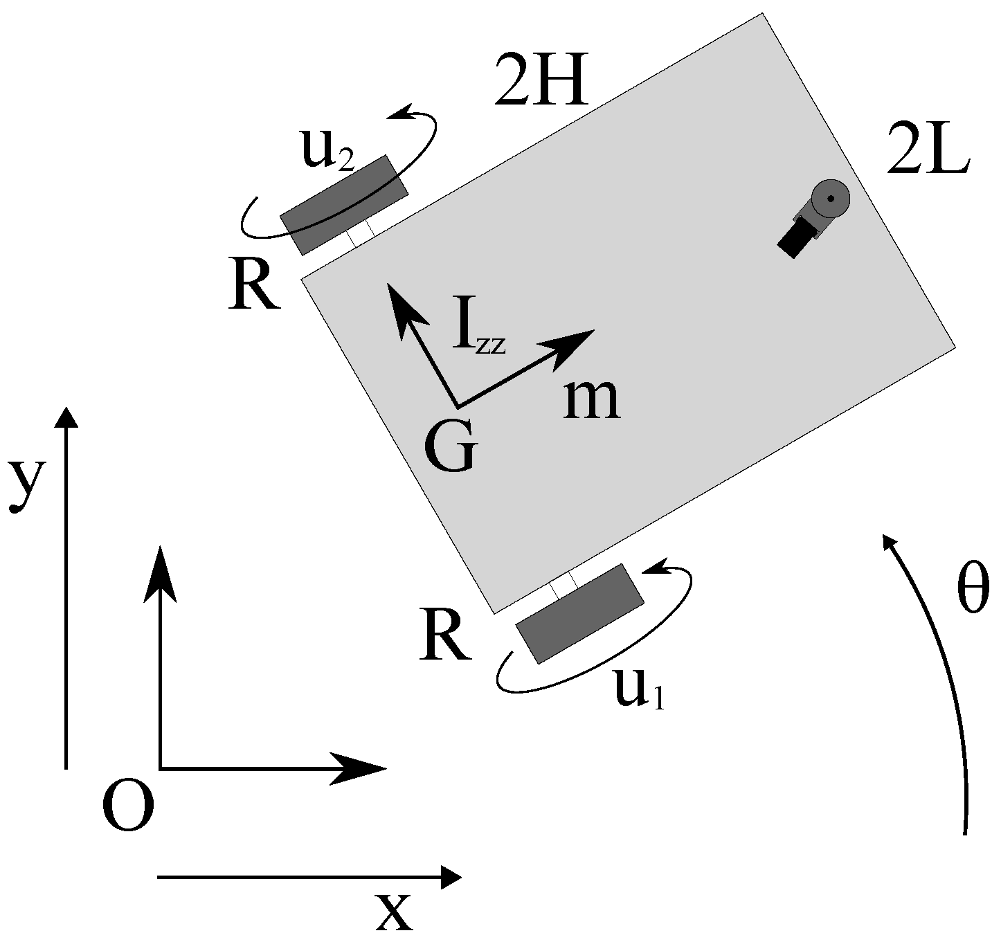
3.1. Unicycle-Like Mobile Robot Model

In this subsection, the description of the unicycle-like mobile robot used as a demonstrative example is presented. A schematic representation of the wheeled mobile robot considered herein is shown in Figure 1.
The dynamical system considered in this subsection is endowed with n b = 3 degrees of freedom. This mechanical system is subjected to a nonlinear force field which mathematically represents the dissipation phenomena. Furthermore, the mobile robot must satisfy a nonholonomic constraint equation which represents the pure rolling condition and, therefore, n c = 1 . Thus, the unicycle-like mobile robot is described by the following symbolic set of equations of motion:
M q ¨ = Q σ + Q r A r q ¨ = b r
where q is the configuration vector of the mobile robot, M represents the mass matrix of the mobile robot, Q σ is the generalized force vector associated with the dissipative effects which influence the dynamic behavior of the mobile robot, Q r identifies the generalized force vector arising from the pure rolling nonholonomic constraint equation that can be explicitly obtained by applying the Udwadia-Kalaba Equations, A r is the pure rolling constraint Jacobian matrix, and b r represents the pure rolling constraint quadratic velocity vector. These vector and matrix quantities are respectively given by:
M = m 0 0 0 m 0 0 0 I z z , Q σ = σ x ˙ σ y ˙ 0 , Q r = m sin ( θ ) θ ˙ cos ( θ ) x ˙ + sin ( θ ) y ˙ m cos ( θ ) θ ˙ cos ( θ ) x ˙ + sin ( θ ) y ˙ 0
and
q = x y θ , A r = sin ( θ ) cos ( θ ) 0 , b r = cos ( θ ) θ ˙ x ˙ + sin ( θ ) θ ˙ y ˙
where m is the robot mass, I z z denotes the robot moment of inertia, σ is the viscous damping coefficient that models the dissipation forces acting on the mobile robot, x represents the abscissa of the robot center of mass, y represents the ordinate of the robot center of mass, and θ is the angular orientation of the mobile robot. In particular, the generalized force vector arising from the pure rolling nonholonomic constraint Q r was explicitly obtained by applying the general form of the Udwadia-Kalaba Equations to the pure rolling constraint equations defined in the standard form described by the vector and matrix quantities A r and b r . To this end, Equation (19) can be effectively used. To achieve this goal, the pure rolling condition of the mobile robot is modeled as a nonholonomic constraint equation assuming that the velocity v G of the robot center of mass G must be orthogonal to the direction vector j associated with the robot wheels for each instant of time. Therefore, the vectors v G and j must be orthogonal for each instant of time to model the pure rolling of the wheeled mobile robot. Thus, one can write:
v G T j = 0
where:
v G = x ˙ y ˙ , j = sin ( θ ) cos ( θ )
Equation (40) represents a nonholonomic constraint equation that involves the generalized configuration vector of the mobile robot q and its time derivative q ˙ . By imposing this nonlinear condition, one obtains an algebraic equation which involves both the system generalized positions and velocities. This algebraic equation cannot be rewritten only in terms of the system generalized configuration vector q . Therefore, the pure rolling condition is a nonholonomic constraint equation. The Udwadia-Kalaba Equations, on the other hand, were used for obtaining in a concise form the generalized force vector Q r starting from the analytical definition of the pure rolling nonholonomic constraint equation given by Equation (40). To achieve this goal, one can effectively employ the following step-by-step derivation. First, the kinetic matrix K r associated with the mobile robot subjected to the pure rolling condition can be computed as follows:
K r = A r M 1 A r T = sin ( θ ) cos ( θ ) 0 1 m 0 0 0 1 m 0 0 0 1 I z z sin ( θ ) cos ( θ ) 0 = 1 m
where A r and b r are the vector and matrix quantities that represent the pure rolling condition in the standard form associated with nonholonomic constraint equations. The constraint feedback matrix F r corresponding to the kinetic matrix K r relative to the pure rolling condition of the mobile robot is given by:
F r = K r + = K r 1 = m
The unconstrained generalized acceleration vector a r obtained in absence of external force fields acting on the mobile robot is a zero vector:
a r = 0
Therefore, the error vector obtained by introducing the unconstrained generalized acceleration vector a r into the pure rolling nonholonomic constraint equation can be readily calculated to yield:
e r = b r A r a r = cos ( θ ) θ ˙ x ˙ + sin ( θ ) θ ˙ y ˙
Finally, one can obtain the generalized force vector Q r associated with the pure rolling condition of the mobile robot as follows:
Q r = A r T F r e r = sin ( θ ) cos ( θ ) 0 m cos ( θ ) θ ˙ x ˙ + sin ( θ ) θ ˙ y ˙ = m sin ( θ ) θ ˙ cos ( θ ) x ˙ + sin ( θ ) y ˙ m cos ( θ ) θ ˙ cos ( θ ) x ˙ + sin ( θ ) y ˙ 0
The explicit calculation of the generalized force vector Q r is one of the main results of this work which allows for performing dynamical simulation by using standard numerical integration techniques based on a sequential marching of the numerical solution on the time grid.

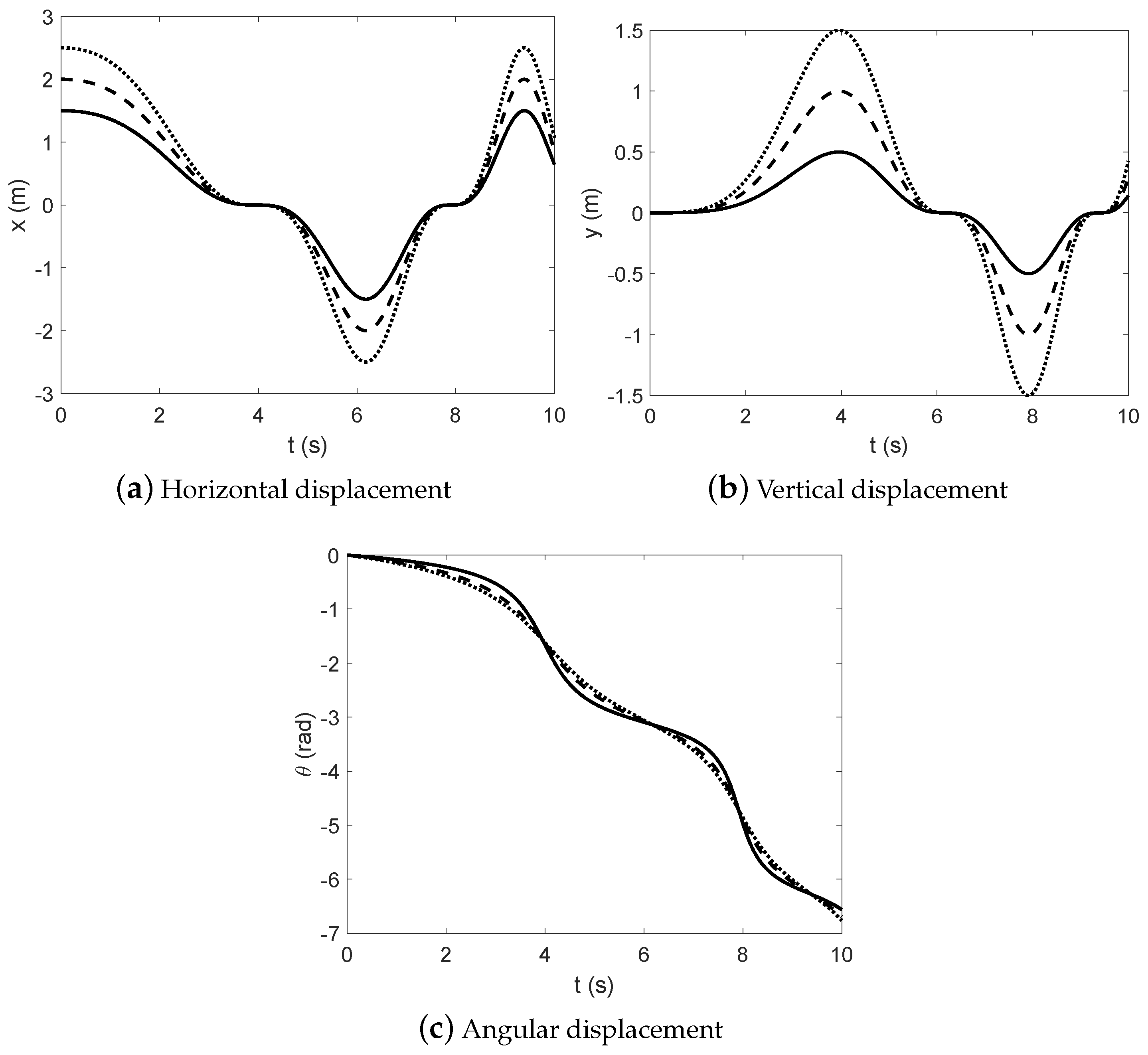
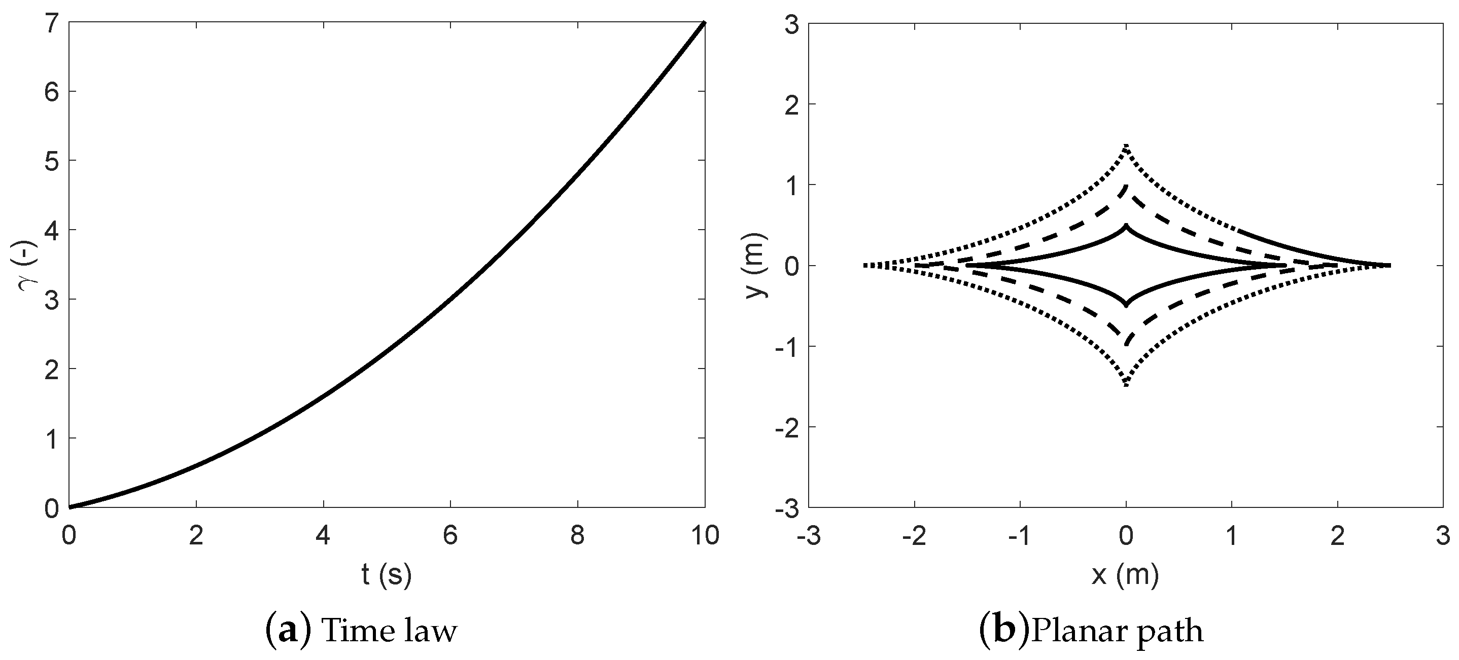
3.2. Nonlinear Trajectory Tracking

In this subsection, the derivation of a nonlinear tracking controller based on the inverse dynamic approach developed in the paper is presented. For this purpose, consider the application of an external control action on the mobile robot having an underactuated structure, which implies the following set of equations of motion:
M q ¨ = Q σ + Q r + B u u
where u is a vector of external control actions and B u denotes an input influence matrix that are respectively given by:
u = u 1 u 2 , B u = cos ( θ ) R cos ( θ ) R sin ( θ ) R sin ( θ ) R L R L R
where the number of the active control actions is n u = 2 , while u 1 is the control torque applied on the right wheel of the mobile robot, u 2 is the control torque applied on the left wheel of the mobile robot, L denotes half the length of the robot axle track, and R corresponds to the radius of the robot wheels. To obtain a nonlinear tracking controller for the mobile robot and, at the same time, to impose the underactuation property of this mechanical system by considering a nonholonomic constraint equation defined at the acceleration level, one can assume the following nonholonomic constraint equations defined in the standard form:
A t q ¨ = b t
where A t is the trajectory tracking constraint Jacobian matrix and b t represents the trajectory tracking constraint quadratic velocity vector. These matrix and vector quantities are respectively defined as:
A t = m R cos ( θ ) m R sin ( θ ) 0 1 0 0 0 0 1 , b t = R cos ( θ ) σ x ˙ m sin ( θ ) θ ˙ cos ( θ ) x ˙ + sin ( θ ) y ˙ + R sin ( θ ) σ y ˙ + m cos ( θ ) θ ˙ cos ( θ ) x ˙ + sin ( θ ) y ˙ ξ ¨ φ ¨
where ξ represents a prescribed function of time for the abscissa x of the robot center of mass and φ denotes a prescribed function of time for the angular orientation θ of the robot chassis, whereas the first equation in these matrix expressions is a mathematical representation of the underactuation requirement which can be readily obtained by applying the Underactuation Equivalence Principle given by Equation (29). These equations are written at the acceleration level and arise from the following set of nonholonomic constraint equations:
m R cos ( θ ) x ¨ m R sin ( θ ) y ¨ = R cos ( θ ) σ x ˙ m sin ( θ ) θ ˙ cos ( θ ) x ˙ + sin ( θ ) y ˙ R sin ( θ ) σ y ˙ + m cos ( θ ) θ ˙ cos ( θ ) x ˙ + sin ( θ ) y ˙ x = ξ θ = φ
By imposing the previous set of constraint equations on the unicycle-like mobile robot, one obtains the generalized force vector associated with the nonlinear controller for the trajectory tracking by means of the Udwadia-Kalaba Equations given by Equation (19). This generalized force vector is denoted with Q t and is given by:
Q t = A t T F t e t = σ x ˙ + m sin ( θ ) θ ˙ cos ( θ ) x ˙ + sin ( θ ) y ˙ + m ξ ¨ tan ( θ ) σ x ˙ + m sin ( θ ) θ ˙ cos ( θ ) x ˙ + sin ( θ ) y ˙ + m ξ ¨ I z z φ ¨
This generalized force vector allows for imposing on the unicycle-like mobile robot a set of control actions suitable for tracking a prescribed state-space trajectory defined in terms of the arbitrary functions ξ and φ . However, it is important to note that the functions ξ and φ , which define the desired state-space trajectory, must be also consistent with the pure rolling condition imposed on the unicycle-like mobile robot.

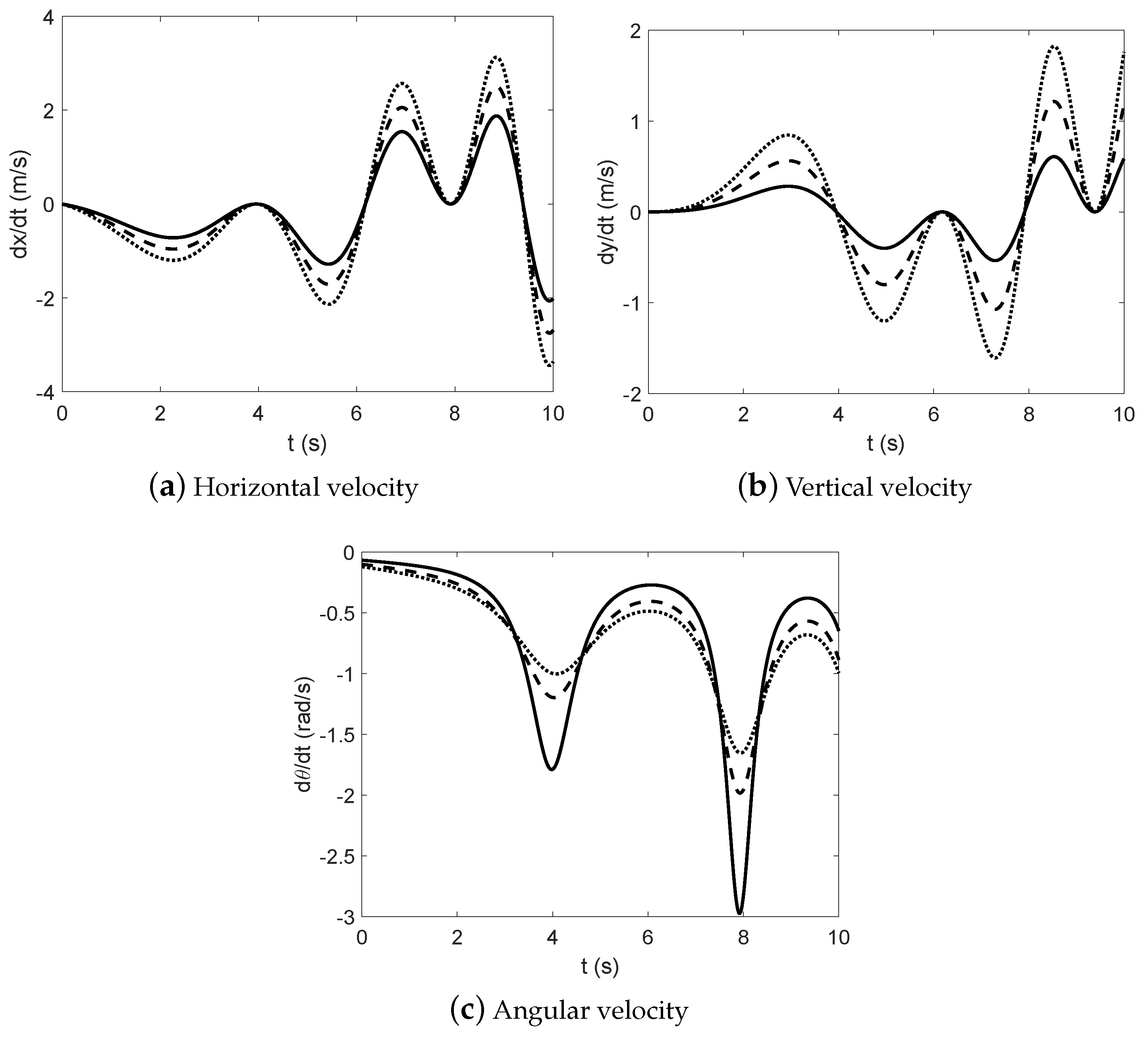
3.3. Dynamic Analysis

In this subsection, the numerical results found using the approach developed in the paper are presented. For this purpose, consider the numerical data for the unicycle-like mobile robot reported in Table 1.
In the dynamic analysis, a time span equal to T = 10 ( s ) is considered and a step size equal to Δ t = 10 3 ( s ) is assumed. The computational algorithm used for performing the time marching of the numerical solution of the equations of motion is the sixth-order Adams-Bashforth method. To demonstrate the effectiveness of the proposed method for performing the tracking controller of the unicycle-like mobile robot, consider the following parametric form for the system path and time law:
ξ = C + a cos 3 ( γ ) η = D + b sin 3 ( γ ) φ = atan 2 ( d η d γ , d ξ d γ ) γ = 1 2 α t 2 + β t + δ
where ξ is the assigned horizontal displacement, η is the assigned vertical displacement, φ is the assigned angular displacement, and γ is the assigned time law. Thus, the time law chosen for the mobile robot is a uniformly accelerated motion whereas the planar curve considered for the path is an astroid. The numerical values of the constant parameters that appear in these equations are respectively defined in Table 2.
To test the performance of the inverse dynamic method developed in this paper in multiple scenarios, three different sets of initial conditions are considered for the unicycle-like mobile robot. For simplicity, the three set of initial conditions considered in this work are respectively labeled with the numbers 1, 2, and 3 as shown in Table 3.
In Table 3, considering a general set of initial conditions labeled with the number i = 1 , 2 , 3 , x 0 i is the initial horizontal displacement, y 0 i represents the initial vertical displacement, θ 0 i denotes the initial angular displacement, u 0 i is the initial horizontal velocity, v 0 i represents the initial vertical velocity, and ω 0 i denotes the initial angular velocity. The resulting horizontal displacement, vertical displacement, and angular displacement of the mechanical system obtained in the dynamical analysis by using the designed tracking control actions are respectively shown in Figure 2a–c.
The time law used for performing the dynamic analysis is represented in Figure 3a, while the planar path of the unicycle-like mobile robot resulting from the application of the control inputs obtained by using the proposed inverse dynamic approach is represented in Figure 3b.
The resulting horizontal velocity, vertical velocity, and angular velocity of the mechanical system obtained in the dynamical analysis by using the designed tracking control actions are respectively shown in Figure 4a–c.
Furthermore, the right and left control actions which allow for performing the tracking control in correspondence of the designed state-space trajectory are respectively shown in Figure 5a,b.
In Figure 2a–c, Figure 3a,b, Figure 4a–c and Figure 5a,b, the solid lines refer to the set of initial conditions labeled with the number 1, the dashed lines refer to the set of initial conditions labeled with the number 2, and the dotted lines refer to the set of initial conditions labeled with the number 3, respectively.

4. Discussion

In this section, a critical discussion of the numerical results obtained in the paper is reported and some directions for future research are provided.

4.1. Performance Analysis

The motion of the mobile robot represented in Figure 2a,b demonstrates that the method proposed in the paper can be effectively used for devising nonlinear control actions for mechanical systems constrained by holonomic as well as nonholonomic constraints. To quantify the performance of the proposed approach, one can compute the deviation of the actual state-space trajectory obtained by using the nonlinear controller from the theoretical state-space trajectory imposed as the reference solution. To this end, the absolute errors between the actual state-space trajectory and the desired state-space trajectory can be used for evaluating the performance of the control method proposed in the paper. The absolute error for the planar path is simply defined as:
e x ( t ) = x ( t ) ξ ( t ) e y ( t ) = y ( t ) η ( t )
where e x ( t ) and e y ( t ) respectively denote the absolute errors of the horizontal and vertical displacements x and y. Figure 6a shows the time evolution of the absolute error related to the horizontal displacement, while Figure 6b shows the time evolution of the absolute error related to the vertical displacement.
In Figure 6a,b, the solid lines refer to the set of initial conditions labeled with the number 1, the dashed lines refer to the set of initial conditions labeled with the number 2, and the dotted lines refer to the set of initial conditions labeled with the number 3, respectively. Furthermore, the root-mean-square deviations between the actual state-space trajectory and the desired state-space trajectory are used in this investigation as a quantitative metric. The root-mean-square deviations are defined as follows:
x R M S = 1 N n = 1 N x ( t n ) ξ ( t n ) 2 y R M S = 1 N n = 1 N y ( t n ) η ( t n ) 2
where x R M S and y R M S respectively denote the RMS deviation of the horizontal and vertical displacements x and y. The numerical results found for the horizontal and vertical root-mean-square deviations are reported in Table 4.
The numerical results found for the root-mean-square deviations are referred to the three sets of initial conditions considered in this research work that are labeled with the numbers 1, 2, and 3. Table 4 shows that the numerical solution obtained in the dynamic simulation involves small deviations from the designed state-space trajectory. These errors are caused by the numerical approximation used for obtaining the numerical solution of the equations of motion which affect each numerical integration scheme suitable for solving nonlinear sets of ordinary differential equations. Therefore, the numerical results found in this section show a good agreement between the actual state-space trajectory obtained using the proposed inverse dynamic method and the desired state-space trajectory arising from a preliminary motion planning phase, thereby demonstrating the effectiveness of the methodology developed in this paper.

4.2. General Considerations

In this paper, the starting point is the analysis of the robot kinematic model, while the complete nonlinear dynamic model of the unicycle robot is subsequently employed for testing the inverse dynamic method proposed in this investigation to obtain an analytical solution for the tracking control problem. Because of the no side-slip condition of the wheel, which is kinematically equivalent to a no-slip condition, the unicycle robot cannot move in the direction of the wheel axis and, therefore, the motion of the robot must take place only in the direction of its heading. This pure rolling condition implies that the velocity vector of the unicycle robot must be parallel to the longitudinal direction of the robot chassis. Therefore, the no side-slip condition must be mathematically modeled as a nonholonomic algebraic equation. In general, mechanical systems subjected to nonholonomic constraints are difficult to control and the main goal of this paper is to provide a general method for addressing this challenge. In this research work, an effective inverse dynamic control method based on the combined application of the Udwadia-Kalaba Equations with the Underactuation Equivalence Principle was developed and tested in the case of a unicycle mobile robot. In principle, the approach developed in the paper can be directly extended to the solution of the control problem of other wheeled mobile robots, such as the bicycle mobile robot, as well as to legged mobile robot. However, these developments will be the objects of future investigations.
The nonlinear control problem of wheeled mobile robots represents a challenging issue. Several effective methods were proposed in the literature for solving this problem [56,57,58,59,60,61,62,63]. However, the main difficulty associated with the nonlinear control approaches employed in the literature for wheeled mobile robots is that they rely on non-standard techniques which cannot be readily extended to other control problems [71,72,73,74]. Unlike the methods already available in the literature, an inverse dynamic method based on the use of the Udwadia-Kalaba Equations was developed in this work. The proposed method is effective, general, and can be easily applied to different control problems related to mobile robots. Furthermore, in principle, the inverse dynamic method developed in this study can be combined with the conventional optimal control method for obtaining the design of a feedforward plus feedback control architecture. This promising combination will be investigated in future research works.
Future research will be devoted to the application of the nonlinear control algorithm developed in this paper to more complex mechanical systems having an underactuated structure and constrained by holonomic as well as nonholonomic algebraic equations. For instance, the immediate extension of this work, which is focused on the stabilization and tracking problem of a unicycle-like mobile robot, is the development of an inverse dynamic computational procedure applied to a bicycle model of a wheeled mobile robot subjected to a set of nonholonomic constraints that analytically define the pure rolling condition of the robot wheels. Moreover, further directions of future research are related to dynamic and control problems of multibody mechanical systems, namely mechanical systems formed by rigid as well as flexible components interconnected by kinematic joints, which comprise many degrees of freedom and represent dynamical systems particularly challenging to mathematically model and computationally analyze. Another important direction for future research works to be explored is the use of the methods of optimal control theory in conjunction with the inverse dynamic approach based on the Udwadia-Kalaba Equations combined with the Underactuation Equivalence Principle developed in this investigation.

5. Summary and Conclusions

The scientific research of the authors is focused on three main areas of interest that are closely related to practical applications in the field of mechanical engineering. The general topics addressed by the investigation of the authors are system identification, nonlinear control, and multibody dynamics [106,107,108,109,110]. System identification is aimed at obtaining a good estimation of the parameters that define a dynamical model of a given mechanical system. Nonlinear control deals with the development of nonlinear control strategies for mechanical systems described by nonlinear mathematical models. Multibody dynamics is a branch of analytical mechanics devoted to the study of the dynamic behavior of articulated systems composed of rigid or flexible bodies constrained by mechanical joints.
This paper is concerned with forward and inverse dynamic problems of wheeled mobile robots having an underactuated structure and is part of a wider research plan inspired by the vision of the authors. In particular, this work is focused on the dynamic and control problem of wheeled mobile robots having a unicycle-like structure. This type of mobile robots represents an important example of a large class of underactuated nonholonomic nonlinear mechanical systems which is used in the field of nonlinear control for testing the effectiveness of new computational algorithms. The method developed in the paper is based on the use of the Udwadia-Kalaba Equations in conjunction with the Underactuation Equivalence Principle. It is shown in this paper that the Udwadia-Kalaba Equations can be employed for deriving the generalized force vector necessary for solving both forward and inverse dynamic problems of nonholonomic mechanical systems. Also, this investigation demonstrates that the Underactuation Equivalence Principle allows for extending the effectiveness of the use of the Udwadia-Kalaba Equations from fully actuated mechanical systems to underactuated mechanical systems. To demonstrate this fact, the nonlinear trajectory tracking problem of a unicycle-like mobile robot is considered in this work as an illustrative example. Dynamical simulations and numerical experiments corroborate the analytical developments obtained in this paper. In particular, the numerical results found for the unicycle robot show a small error between the desired trajectory and the actual trajectory followed by the mobile robot.
In future research works, the method developed in this paper will be used as an open-loop (feedforward) control law and will be combined with the optimal control technique that is useful for the design of compensator controllers based on a closed-loop (feedback) architecture. Furthermore, the method developed in this work will be applied to the solution of inverse dynamic problems of more complex mechanical systems like, for example, the bicycle model of a wheeled mobile robot.

Author Contributions

This research paper was principally developed by the first author (C.M.P.). The detailed review carried out by the second author (D.G.) considerably improved the quality of the work.

Funding

This research work received no external funding.

Conflicts of Interest

The authors declare no conflicts of interest.

References

  1. Juang, J.N.; Phan, M.Q. Identification and Control of Mechanical Systems; Cambridge University Press: New York, NY, USA, 2001. [Google Scholar]
  2. Villecco, F. On the Evaluation of Errors in the Virtual Design of Mechanical Systems. Machines 2018, 6, 36. [Google Scholar] [CrossRef]
  3. Sena, P.; Attianese, P.; Pappalardo, M.; Villecco, F. FIDELITY: Fuzzy inferential diagnostic engine for on-line support to physicians. In Proceedings of the 4th International Conference on the Development of Biomedical Engineering in Vietnam, Ho Chi Minh City, Vietnam, 8–10 January 2012; pp. 396–400. [Google Scholar]
  4. Ghomshei, M.; Villecco, F.; Porkhial, S.; Pappalardo, M. Complexity in Energy Policy: A Fuzzy Logic Methodology. In Proceedings of the 6th International Conference on Fuzzy Systems and Knowledge Discovery, Tianjin, China, 14–16 August 2009; IEEE: Los Alamitos, CA, USA, 2009; Volume 7, pp. 128–131. [Google Scholar]
  5. Zhai, Y.; Liu, L.; Lu, W.; Li, Y.; Yang, S.; Villecco, F. The Application of Disturbance Observer to Propulsion Control of Sub-mini Underwater Robot. In Proceedings of the ICCSA 2010 International Conference on Computational Science and Its Applications, Fukuoka, Japan, 23–26 March 2010; pp. 590–598. [Google Scholar]
  6. Sena, P.; D’Amore, M.; Pappalardo, M.; Pellegrino, A.; Fiorentino, A.; Villecco, F. Studying the Influence of Cognitive Load on Driver’s Performances by a Fuzzy Analysis of Lane Keeping in a Drive Simulation. IFAC Proc. Vol. 2013, 46, 151–156. [Google Scholar] [CrossRef]
  7. Ghomshei, M.; Villecco, F. Energy Metrics and Sustainability. In Proceedings of the International Conference on Computational Science and Its Applications, Seoul, Korea, 29 June–2 July 2009; pp. 693–698. [Google Scholar]
  8. Sena, P.; Attianese, P.; Carbone, F.; Pellegrino, A.; Pinto, A.; Villecco, F. A Fuzzy Model to Interpret Data of Drive Performances from Patients with Sleep Deprivation. Comput. Math. Methods Med. 2012, 2012, 868410. [Google Scholar] [CrossRef] [PubMed]
  9. Zhang, Y.; Li, Z.; Gao, J.; Hong, J.; Villecco, F.; Li, Y. A method for designing assembly tolerance networks of mechanical assemblies. Math. Probl. Eng. 2012, 2012, 513958. [Google Scholar] [CrossRef]
  10. Villecco, F.; Pellegrino, A. Evaluation of Uncertainties in the Design Process of Complex Mechanical Systems. Entropy 2017, 19, 475. [Google Scholar] [CrossRef]
  11. Pellegrino, A.; Villecco, F. Design Optimization of a Natural Gas Substation with Intensification of the Energy Cycle. Math. Probl. Eng. 2010, 2010, 294102. [Google Scholar] [CrossRef]
  12. Sequenzia, G.; Fatuzzo, G.; Oliveri, S.M.; Barbagallo, R. Interactive re-design of a novel variable geometry bicycle saddle to prevent neurological pathologies. Int. J. Int. Des. Man. 2016, 10, 165–172. [Google Scholar] [CrossRef]
  13. Barbagallo, R.; Sequenzia, G.; Cammarata, A.; Oliveri, S.M.; Fatuzzo, G. Redesign and multibody simulation of a motorcycle rear suspension with eccentric mechanism. Int. J. Int. Des. Man. 2018, 12, 517–524. [Google Scholar] [CrossRef]
  14. Barbagallo, R.; Sequenzia, G.; Oliveri, S.M.; Cammarata, A. Dynamics of a high-performance motorcycle by an advanced multibody/control co-simulation. Proc. Inst. Mech. Eng. Part K J. Eng. 2016, 230, 207–221. [Google Scholar] [CrossRef]
  15. Cammarata, A.; Sequenzia, G.; Oliveri, S.M.; Fatuzzo, G. Modified chain algorithm to study planar compliant mechanisms. Int. J. Int. Des. Man. 2016, 10, 191–201. [Google Scholar] [CrossRef]
  16. Oliveri, S.M.; Sequenzia, G.; Calí, M. Flexible multibody model of desmodromic timing system. Mech. Based Des. Struct. 2009, 37, 15–30. [Google Scholar] [CrossRef]
  17. Barbagallo, R.; Sequenzia, G.; Cammarata, A.; Oliveri, S.M. An integrated approach to design an innovative motorcycle rear suspension with eccentric mechanism. In Advances on Mechanics, Design Engineering and Manufacturing; Springer: Cham, Switzerland, 2017; pp. 609–619. [Google Scholar]
  18. Calí, M.; Oliveri, S.M.; Sequenzia, G. Geometric modeling and modal stress formulation for flexible multi-body dynamic analysis of crankshaft. In Proceedings of the 25th Conference and Exposition on Structural Dynamics 2007, Orlando, FL, USA, 19–22 February 2007; pp. 1–9. [Google Scholar]
  19. Cammarata, A. A novel method to determine position and orientation errors in clearance-affected overconstrained mechanisms. Mech. Mach. Theory 2017, 118, 247–264. [Google Scholar] [CrossRef]
  20. Cammarata, A.; Calió, I.; Greco, A.; Lacagnina, M.; Fichera, G. Dynamic stiffness model of spherical parallel robots. J. Sound Vib. 2016, 384, 312–324. [Google Scholar] [CrossRef]
  21. Callegari, M.; Cammarata, A.; Gabrielli, A.; Sinatra, R. Kinematics and dynamics of a 3-CRU spherical parallel robot. In Proceedings of the ASME 2007 International Design Engineering Technical Conferences and Computers and Information in Engineering Conference, Las Vegas, NV, USA, 4–7 September 2007; pp. 933–941. [Google Scholar]
  22. Cammarata, A.; Lacagnina, M.; Sequenzia, G. Alternative elliptic integral solution to the beam deflection equations for the design of compliant mechanisms. Int. J. Interact. Des. Manuf. (IJIDeM) 2018, 1–7. [Google Scholar] [CrossRef]
  23. Cammarata, A.; Sinatra, R.; Maddio, P.D. A Two-Step Algorithm for the Dynamic Reduction of Flexible Mechanisms. In Mechanism Design for Robotics; Springer: Cham, Switzerland, 2018; pp. 25–32. [Google Scholar]
  24. Muscat, M.; Cammarata, A.; Maddio, P.D.; Sinatra, R. Design and development of a towfish to monitor marine pollution. Euro-Mediterr. J. Environ. Integr. 2018, 3, 11. [Google Scholar] [CrossRef] [Green Version]
  25. Cammarata, A.; Sinatra, R. On the elastostatics of spherical parallel machines with curved links. In Recent Advances in Mechanism Design for Robotics; Springer: Cham, Switzerland, 2015; pp. 347–356. [Google Scholar]
  26. Cammarata, A.; Lacagnina, M.; Sinatra, R. Dynamic simulations of an airplane-shaped underwater towed vehicle marine. In Proceedings of the 5th International Conference on Computational Methods in Marine Engineering, Hamburg, Germany, 29–31 May 2013; pp. 830–841, Code 101673. ISBN 978-849414074-7. [Google Scholar]
  27. Cammarata, A.; Lacagnina, M.; Sinatra, R. Closed-form solutions for the inverse kinematics of the Agile Eye with constraint errors on the revolute joint axes. In Proceedings of the 2016 IEEE/RSJ International Conference on Intelligent Robots and Systems (IROS), Daejeon, Korea, 9–14 October 2016; pp. 317–322. [Google Scholar]
  28. Cammarata, A.; Angeles, J.; Sinatra, R. Kinetostatic and inertial conditioning of the McGill Schonflies-motion generator. Adv. Mech. Eng. 2010, 2, 186203. [Google Scholar] [CrossRef]
  29. Cammarata, A. Unified formulation for the stiffness analysis of spatial mechanisms. Mech. Mach. Theory 2016, 105, 272–284. [Google Scholar] [CrossRef]
  30. Cammarata, A. Optimized design of a large-workspace 2-DOF parallel robot for solar tracking systems. Mech. Mach. Theory 2015, 83, 175–186. [Google Scholar] [CrossRef]
  31. Tanev, T.K.; Cammarata, A.; Marano, D.; Sinatra, R. Elastostatic model of a new hybrid minimally-invasive-surgery robot. In Proceedings of the 14th IFToMM World Congress, Taipei, Taiwan, 25–30 October 2015. [Google Scholar]
  32. Reinhart, R.F.; Shareef, Z.; Steil, J.J. Hybrid Analytical and Data-Driven Modeling for Feed-Forward Robot Control. Sensors 2017, 17, 311. [Google Scholar] [CrossRef] [PubMed]
  33. Diez, S.; Hoefling, A.; Theato, P.; Pauer, W. Mechanical and Electrical Properties of Sulfur-Containing Polymeric Materials Prepared via Inverse Vulcanization. Polymers 2017, 9, 59. [Google Scholar] [CrossRef]
  34. Qin, C.; Zhang, C.; Lu, H. H-Shaped Multiple Linear Motor Drive Platform Control System Design Based on an Inverse System Method. Energies 2017, 10, 1990. [Google Scholar] [CrossRef]
  35. Duan, X.; Yang, Y.; Cheng, B. Modeling and Analysis of a 2-DOF Spherical Parallel Manipulator. Sensors 2016, 16, 1485. [Google Scholar] [CrossRef]
  36. Garcia-Murillo, M.A.; Sanchez-Alonso, R.E.; Gallardo-Alvarado, J. Kinematics and Dynamics of a Translational Parallel Robot Based on Planar Mechanisms. Machines 2016, 4, 22. [Google Scholar] [CrossRef]
  37. Zhuge, C.; Cai, Y.; Tang, Z. A novel dynamic obstacle avoidance algorithm based on Collision time histogram. Chin. J. Electron. 2017, 26, 522–529. [Google Scholar] [CrossRef]
  38. Khan, M.; Hassan, S.; Ahmed, S.I.; Iqbal, J. Stereovision-based real-time obstacle detection scheme for Unmanned Ground Vehicle with steering wheel drive mechanism. In Proceedings of the 2017 International Conference on Communication, Computing and Digital Systems, C-CODE 2017, Islamabad, Pakistan, 8–9 March 2017; pp. 380–385. [Google Scholar]
  39. Ji, J.; Khajepour, A.; Melek, W.W.; Huang, Y. Path planning and tracking for vehicle collision avoidance based on model predictive control with multiconstraints. IEEE Trans. Veh. Technol. 2017, 66, 952–964. [Google Scholar] [CrossRef]
  40. Wang, Y.; Goila, A.; Shetty, R.; Heydari, M.; Desai, A.; Yang, H. Obstacle Avoidance Strategy and Implementation for Unmanned Ground Vehicle Using LIDAR. SAE Int. J. Commer. Veh. 2017, 10, 50–55. [Google Scholar] [CrossRef]
  41. Lee, S.; Cho, S.; Sim, S.; Kwak, K.; Park, Y.W.; Cho, K. A dynamic zone estimation method using cumulative voxels for autonomous driving. Int. J. Adv. Robot. Syst. 2017, 14. [Google Scholar] [CrossRef] [Green Version]
  42. Al-Mayyahi, A.; Wang, W.; Hussein, A.A.; Birch, P. Motion control design for unmanned ground vehicle in dynamic environment using intelligent controller. Int. J. Intell. Comput. Cybern. 2017, 10, 530–548. [Google Scholar] [CrossRef] [Green Version]
  43. Al-Mayyahi, A.; Wang, W.; Birch, P. Adaptive neuro-fuzzy technique for autonomous ground vehicle navigation. Robotics 2014, 3, 349–370. [Google Scholar] [CrossRef]
  44. Van Pham, H.; Moore, P. Robot Coverage Path Planning under Uncertainty Using Knowledge Inference and Hedge Algebras. Machines 2018, 6, 46. [Google Scholar] [CrossRef]
  45. Zhang, H.Y.; Lin, W.M.; Chen, A.X. Path Planning for the Mobile Robot: A Review. Symmetry 2018, 10, 450. [Google Scholar] [CrossRef]
  46. Ravankar, A.; Ravankar, A.; Kobayashi, Y.; Hoshino, Y.; Peng, C.C. Path Smoothing Techniques in Robot Navigation: State-of-the-Art, Current and Future Challenges. Sensors 2018, 18, 3170. [Google Scholar] [CrossRef]
  47. Kim, J.; Park, J.; Chung, W. Self-Diagnosis of Localization Status for Autonomous Mobile Robots. Sensors 2018, 18, 3168. [Google Scholar] [CrossRef]
  48. Shih, C.L.; Lin, L.C. Trajectory Planning and Tracking Control of a Differential-Drive Mobile Robot in a Picture Drawing Application. Robotics 2017, 6, 17. [Google Scholar] [CrossRef]
  49. Milosavljevic, B.; Pesic, R.; Dasic, P. Binary logistic regression modeling of idle CO emissions in order to estimate predictors influences in old vehicle park. Math. Prob. Eng. 2015, 463158. [Google Scholar] [CrossRef]
  50. Serifi, V.; Dasic, P.; Jecmenica, R.; Labovic, D. Functional and Information Modeling of Production using IDEF Methods. Strojniski Vestnik/J. Mech. Eng. 2009, 55, 131–140. [Google Scholar]
  51. Dasic, P.; Franek, F.; Assenova, E.; Radovanovic, M. International Standardization and Organizations in the Field of Tribology. Ind. Lubr. Tribol. 2003, 55, 287–291. [Google Scholar] [CrossRef]
  52. Dasic, P. Determination of Reliability of Ceramic Cutting Tools on the basis of Comparative Analysis of Different Functions Distribution. Int. J. Qual. Reliab. Manag. 2001, 18, 431–443. [Google Scholar]
  53. De Simone, M.C.; Rivera, Z.B.; Guida, D. Obstacle Avoidance System for Unmanned Ground Vehicles by Using Ultrasonic Sensors. Machines 2018, 6, 18. [Google Scholar] [CrossRef]
  54. De Simone, M.C.; Russo, S.; Rivera, Z.B.; Guida, D. Multibody model of a UAV in presence of wind fields. In Proceedings of the 2017 International Conference on Control, Artificial Intelligence, Robotics & Optimization (ICCAIRO), Prague, Czech Republic, 20–22 May 2017; pp. 83–88. [Google Scholar]
  55. De Simone, M.C.; Guida, D. Identification and Control of a Unmanned Ground Vehicle By using Arduino. UPB Sci. Bull. Ser. D 2018, 80, 141–154. [Google Scholar]
  56. Rajashekaraiah, G.; Sevil, H.E.; Dogan, A. PTEM based moving obstacle detection and avoidance for an unmanned ground vehicle. In Proceedings of the ASME 2017 Dynamic Systems and Control Conference, Tysons, VA, USA, 11–13 October 2017. [Google Scholar]
  57. Zhang, M.; Jasiobedzki, P. Unobtrusive and assistive obstacle avoidance for tele-operation of ground vehicles. In Proceedings of the SPIE—The International Society for Optical Engineering, Trieste, Italy, 31 May 2017; p. 10195. [Google Scholar]
  58. Giesbrecht, J.; Ng, H.-K.; Zhang, M.; Tang, J.; Bondy, M.; Jasiobedzki, P. Safeguarding autonomy through intelligent shared control. In Proceedings of the SPIE—The International Society for Optical Engineering, San Francisco, CA, USA, 28 January–2 February 2017; p. 10195. [Google Scholar]
  59. Mohammadi, S.S.; Khaloozadeh, H. Optimal motion planning of unmanned ground vehicle using SDRE controller in the presence of obstacles. In Proceedings of the 4th International Conference on Control, Instrumentation, and Automation, ICCIA, Qazvin, Iran, 27–28 January 2016; pp. 167–171. [Google Scholar]
  60. Tee Kit Tsun, M.; Lau, B.T.; Siswoyo Jo, H. An Improved Indoor Robot Human-Following Navigation Model Using Depth Camera, Active IR Marker and Proximity Sensors Fusion. Robotics 2018, 7, 4. [Google Scholar] [CrossRef]
  61. Gonzalez, A.; Olazagoitia, J.L.; Vinolas, J. A Low-Cost Data Acquisition System for Automobile Dynamics Applications. Sensors 2018, 18, 366. [Google Scholar] [CrossRef]
  62. Negrete, J.C.; Kriuskova, E.R.; Cantens, G.D.J.L.; Avila, C.I.Z.; Hernandez, G.L. Arduino Board in the Automation of Agriculture in Mexico, a Review. Int. J. 2018, 8, 52–68. [Google Scholar] [CrossRef]
  63. Li, B.; Liu, H.; Zhang, J.; Zhao, X.; Zhao, B. Small UAV autonomous localization based on multiple sensors fusion. In Proceedings of the 2017 IEEE 2nd Advanced Information Technology, Electronic and Automation Control Conference, IAEAC, Chongqing, China, 25–26 March 2017; pp. 296–303. [Google Scholar]
  64. Sharifzadeh, M.; Pisaturo, M.; Farnam, A.; Senatore, A. Joint structure for the real-time estimation and control of automotive dry clutch engagement. IFAC-PapersOnLine 2018, 51, 1062–1067. [Google Scholar] [CrossRef]
  65. Sharifzadeh, M.; Farnam, A.; Senatore, A.; Timpone, F.; Akbari, A. Delay-dependent criteria for robust dynamic stability control of articulated vehicles. Mech. Mach. Sci. 2018, 49, 424–432. [Google Scholar]
  66. Senatore, A.; Pisaturo, M.; Sharifzadeh, M. Real time Identification of Automotive Dry Clutch Frictional Characteristics Using Trust Region Methods. In Proceedings of the 23rd Conference of the Italian Association of Theoretical and Applied Mechanics, Salerno, Italy, 4–7 September 2017; Volume 4, pp. 526–534. [Google Scholar]
  67. Sharifzadeh, M.; Timpone, F.; Farnam, A.; Senatore, A.; Akbari, A. Tyre-road adherence conditions estimation for intelligent vehicle safety applications. In Advances in Italian Mechanism Science; Springer: Cham, Switzerland, 2017; pp. 389–398. [Google Scholar]
  68. Strano, S.; Terzo, M. Actuator Dynamics Compensation for Real-time Hybrid Simulation: An Adaptive Approach by means of a Nonlinear Estimator. Nonlinear Dyn. 2016, 85, 2353–2368. [Google Scholar] [CrossRef]
  69. Strano, S.; Terzo, M. Accurate State Estimation for a Hydraulic Actuator via a SDRE Nonlinear Filter. Mech. Syst. Signal Process. 2016, 75, 576–588. [Google Scholar] [CrossRef]
  70. Strano, S.; Terzo, M. A SDRE-based Tracking Control for a Hydraulic Actuation System. Mech. Syst. Signal Process. 2015, 60, 715–726. [Google Scholar] [CrossRef]
  71. Gupta, P.; Sinha, N.K. Modeling robot dynamics using dynamic neural networks. IFAC Proc. Vol. 1997, 30, 755–759. [Google Scholar] [CrossRef]
  72. Huang, S.N.; Tan, K.K.; Lee, T.H. Adaptive friction compensation using neural network approximations. IEEE Trans. Syst. Man Cybern. Part C (Appl. Rev.) 2000, 30, 551–557. [Google Scholar] [CrossRef]
  73. Fierro, R.; Lewis, F.L. Control of a nonholonomic mobile robot using neural networks. IEEE Trans. Neural Netw. 1998, 9, 589–600. [Google Scholar] [CrossRef]
  74. Nagata, S.; Sekiguchi, M.; Asakawa, K. Mobile robot control by a structured hierarchical neural network. IEEE Control Syst. Mag. 1990, 10, 69–76. [Google Scholar] [CrossRef]
  75. Siciliano, B.; Sciavicco, L.; Villani, L.; Oriolo, G. Robotics: Modelling, Planning and Control; Springer Science and Business Media: Berlin, Germany, 2010. [Google Scholar]
  76. Siciliano, B.; Khatib, O. Springer Handbook of Robotics; Springer: Berlin, Germany, 2016. [Google Scholar]
  77. Lee, T.C.; Song, K.T.; Lee, C.H.; Teng, C.C. Tracking control of unicycle-modeled mobile robots using a saturation feedback controller. IEEE Trans. Control Syst. Technol. 2001, 9, 305–318. [Google Scholar]
  78. Zhang, C.; Arnold, D.; Ghods, N.; Siranosian, A.; Krstic, M. Source seeking with non-holonomic unicycle without position measurement and with tuning of forward velocity. Syst. Control Lett. 2007, 56, 245–252. [Google Scholar] [CrossRef]
  79. Noijen, S.P.M.; Lambrechts, P.F.; Nijmeijer, H. An observer-controller combination for a unicycle mobile robot. Int. J. Control 2005, 78, 81–87. [Google Scholar] [CrossRef] [Green Version]
  80. De Simone, M.C.; Guida, D. On the development of a low-cost device for retrofitting tracked vehicles for autonomous navigation. In Proceedings of the 23rd Conference of the Italian Association of Theoretical and Applied Mechanics, Salerno, Italy, 4–7 September 2017; Volume 4, pp. 71–82. [Google Scholar]
  81. De Simone, M.C.; Guida, D. Control design for an under-actuated UAV model. FME Trans. 2018, 46, 443–452. [Google Scholar]
  82. Dasic, P.; Natsis, A.; Petropoulos, G. Models of Reliability for Cutting Tools: Examples in Manufacturing and Agricultural Engineering. Strojniski Vestnik/J. Mech. Eng. 2008, 54, 122–130. [Google Scholar]
  83. Dasic, P.; Dasic, J.; Crvenkovic, B. Service Models for Cloud Computing: Search as a Service (SaaS). Int. J. Eng. Technol. 2016, 8, 2366–2373. [Google Scholar] [CrossRef]
  84. Dasic, P.; Dasic, J.; Crvenkovic, B. Applications of Access Control as a Service for Software Security. Int. J. Ind. Eng. Manag. (IJIEM) 2016, 7, 111–116. [Google Scholar]
  85. Dasic, P. Comparative analysis of different regression models of the surface roughness in finishing turning of hardened steel with mixed ceramic cutting tools. J. Res. Dev. Mech. Ind. 2013, 5, 101–180. [Google Scholar]
  86. Meirovitch, L. Methods of Analytical Dynamics; Courier Corporation: Chelmsford, MA, USA, 2010. [Google Scholar]
  87. Bauchau, O.A. Flexible Multibody Dynamics; Springer Science and Business Media: Berlin, Germany, 2010. [Google Scholar]
  88. Shabana, A.A.; Zaazaa, K.E.; Sugiyama, H. Railroad Vehicle Dynamics: A Computational Approach; CRC Press: Boca Raton, FL, USA, 2010. [Google Scholar]
  89. Shabana, A.A. Dynamics of Multibody Systems; Cambridge University Press: Cambridge, UK, 2013. [Google Scholar]
  90. Garcia De Jalon, J.G.; Bayo, E. Kinematic and Dynamic Simulation of Multibody Systems: The Real-Time Challenge; Springer: Berlin, Germany, 2012. [Google Scholar]
  91. Schutte, A.; Udwadia, F. New Approach to the Modeling of Complex Multibody Dynamical Systems. J. Appl. Mech. 2011, 78, 021018. [Google Scholar] [CrossRef]
  92. Marques, F.; Souto, A.P.; Flores, P. On the Constraints Violation in Forward Dynamics of Multibody Systems. Multibody Syst. Dyn. 2017, 39, 385–419. [Google Scholar] [CrossRef]
  93. Udwadia, F.E. Equations of Motion for Constrained Multibody Systems and Their Control. J. Optim. Theory Appl. 2005, 127, 627–638. [Google Scholar] [CrossRef]
  94. Udwadia, F.E. Optimal tracking control of nonlinear dynamical systems. Proc. R. Soc. Lond. A Math. Phys. Eng. Sci. 2008, 464, 2341–2363. [Google Scholar] [CrossRef] [Green Version]
  95. Udwadia, F.E.; Kalaba, R.E. Analytical Dynamics: A New Approach; Cambridge University Press: Cambridge, UK, 2007. [Google Scholar]
  96. Lanczos, C. The Variational Principles of Mechanics; Courier Corporation: Chelmsford, MA, USA, 2012. [Google Scholar]
  97. Shabana, A.A. Computational Continuum Mechanics, 3rd ed.; John Wiley and Sons: Hoboken, NJ, USA, 2018. [Google Scholar]
  98. Shabana, A.A. Computational Dynamics, 2nd ed.; John Wiley and Sons: Hoboken, NJ, USA, 2009. [Google Scholar]
  99. Meirovitch, L. Fundamentals of Vibrations; Waveland Press: Long Grove, IL, USA, 2010. [Google Scholar]
  100. Flannery, M.R. The Enigma of Nonholonomic Constraints. Am. J. Phys. 2005, 73, 265–272. [Google Scholar] [CrossRef]
  101. Udwadia, F.E.; Wanichanon, T. On General Nonlinear Constrained Mechanical Systems. Numer. Algebra Control Optim 2013, 3, 425–443. [Google Scholar] [CrossRef]
  102. Pennestrí, E.; Valentini, P.P.; De Falco, D. An Application of the Udwadia-Kalaba Dynamic Formulation to Flexible Multibody Systems. J. Frankl. Inst. 2010, 347, 173–194. [Google Scholar] [CrossRef]
  103. De Falco, D.; Pennestrí, E.; Vita, L. Investigation of the Influence of Pseudoinverse Matrix Calculations on Multibody Dynamics Simulations by means of the Udwadia-Kalaba Formulation. J. Aerosp. Eng. 2009, 22, 365–372. [Google Scholar] [CrossRef]
  104. Udwadia, F.E.; Weber, H.I.; Leitmann, G. Dynamical Systems and Control; CRC Press: Boca Raton, FL, USA, 2016. [Google Scholar]
  105. Fantoni, I.; Lozano, R. Non-Linear Control for Underactuated Mechanical Systems; Springer Science and Business Media: Berlin, Germany, 2002. [Google Scholar]
  106. De Simone, M.C.; Guida, D. Modal coupling in presence of dry friction. Machines 2018, 6, 8. [Google Scholar] [CrossRef]
  107. De Simone, M.C.; Rivera, Z.B.; Guida, D. Finite element analysis on squeal-noise in railway applications. FME Trans. 2018, 46, 93–100. [Google Scholar] [Green Version]
  108. De Simone, M.C.; Guida, D. Object Recognition by Using Neural Networks For Robotics Precision Agriculture Application. Eng. Lett. 2018, in press. [Google Scholar]
  109. Concilio, A.; De Simone, M.C.; Rivera, Z.B.; Guida, D. A new semi-active suspension system for racing vehicles. FME Trans. 2017, 45, 578–584. [Google Scholar] [CrossRef] [Green Version]
  110. Quatrano, A.; De Simone, M.C.; Rivera, Z.B.; Guida, D. Development and implementation of a control system for a retrofitted CNC machine by using Arduino. FME Trans. 2017, 45, 565–571. [Google Scholar] [CrossRef]
Figure 1. Unicycle-like mobile robot.
Machines 07 00005 g001
Figure 2. Robot displacement. Initial conditions 1 (solid lines), initial conditions 2 (dashed lines), initial conditions 3 (dotted lines).
Machines 07 00005 g002
Figure 3. Robot trajectory. Initial conditions 1 (solid lines), initial conditions 2 (dashed lines), initial conditions 3 (dotted lines).
Machines 07 00005 g003
Figure 4. Robot velocity. Initial conditions 1 (solid lines), initial conditions 2 (dashed lines), initial conditions 3 (dotted lines).
Machines 07 00005 g004
Figure 5. Control actions. Initial conditions 1 (solid lines), initial conditions 2 (dashed lines), initial conditions 3 (dotted lines).
Machines 07 00005 g005
Figure 6. Displacement absolute errors. Initial conditions 1 (solid lines), initial conditions 2 (dashed lines), initial conditions 3 (dotted lines).
Machines 07 00005 g006
Table 1. Mobile robot data.
DescriptionsSymbolsData (Units)
Half Length of the Axle TrackL 0.15 ( m )
Radius of the WheelsR 0.025 ( m )
Robot Massm 3 ( kg )
Robot Moment of Inertia I z z 0.0625 ( kg × m 2 )
Viscous Damping Coefficient σ 0.1 ( kg / s )
Table 2. State-space trajectory parameters.
DescriptionsSymbolsData (Units)
Path parameterC 0 ( m )
Path parameterD 0 ( m )
Path parametera 2.0 ( m )
Path parameterb 1.0 ( m )
Time law parameter α 0.1 ( s 2 )
Time law parameter β 0.2 ( s 1 )
Time law parameter δ 0 ( )
Table 3. Sets of initial conditions.
DescriptionsSymbolsData (Units)
Initial horizontal displacement x 0 1 , x 0 2 , x 0 3 1.5 ( m ) , 2.0 ( m ) , 2.5 ( m )
Initial vertical displacement y 0 1 , y 0 2 , y 0 3 0 ( m ) , 0 ( m ) , 0 ( m )
Initial angular displacement θ 0 1 , θ 0 2 , θ 0 3 0 ( rad ) , 0 ( rad ) , 0 ( rad )
Initial horizontal velocity u 0 1 , u 0 2 , u 0 3 0 ( m / s ) , 0 ( m / s ) , 0 ( m / s )
Initial vertical velocity v 0 1 , v 0 2 , v 0 3 0 ( m / s ) , 0 ( m / s ) , 0 ( m / s )
Initial angular velocity ω 0 1 , ω 0 2 , ω 0 3 0.0667 ( rad / s ) , 0.1 ( rad / s ) , 0.12 ( rad / s )
Table 4. State-space trajectory root-mean-square deviations for different sets of initial conditions.
DescriptionsSymbolsData (Units)
Horizontal displacement RMS x R M S 1 , x R M S 2 , x R M S 3 1.684 × 10 10 ( m ) , 2.246 × 10 10 ( m ) , 2.807 × 10 10 ( m )
Vertical displacement RMS y R M S 1 , y R M S 2 , y R M S 3 1.558 × 10 8 ( m ) , 4.248 × 10 8 ( m ) , 7.094 × 10 8 ( m )

