1. Introduction
The engineering and social systems that exist today are often described by high-dimensional and complex mathematical models, such as communication networks, power systems, and transportation. Describing and understanding these systems often necessitate the use of sophisticated mathematical models. These high-dimensional models capture the intricate interactions between various components and factors. Analyzing the stability of such systems is a daunting challenge due to the enormous amount of information that needs to be processed. To address this complexity, researchers have proposed an approach called the interconnected systems (IS) [
1,
2]. By using IS, the complexity of message processing can be effectively reduced. In recent years, many experts and researchers have made great efforts toward the development of IS [
3,
4,
5]. They explore various applications and domains aiming to exploit the potential of this paradigm. For example, the application of disturbance observer-based control in IS has been thoroughly studied [
6]. In another study [
7], the authors delved into the analysis of wind farms using the IS method. Furthermore, the detectability of cyber attacks in interconnected systems has been extensively studied [
8]. To further improve the accuracy and completeness of physical modeling, the concept of an interconnected system has been extended to include the descriptor interconnect system (DIS). The use of descriptor systems allows for a more precise and comprehensive description of bodily behavior [
9]. However, it is important to note that analyzing the stability of descriptor systems presents unique challenges, such as addressing regularity and causality issues [
10]. Despite these challenges, researchers have made remarkable progress in the field of DIS. Several important discoveries and contributions have been reported, elucidating important aspects of stability and stability [
11], sliding mode control [
12], and decentralized static output tracking control [
13], among other important developments.
On the other hand, most physical systems are nonlinear forms, which brings great difficulties in analyzing the stability of the system. Over the past few years, T-S FM [
14,
15] has been considered to be one of the most effective techniques for effectively transforming a nonlinear system into a set of linear subsystems. The T-S FM divides a complex system into a set of smaller subsystems, with each subsystem represented by an if-then rule. These rules consist of two parts: the antecedent, which describes the system inputs using fuzzy sets, and the consequent, which represents the mathematical function of the system outputs. By using fuzzy logic and fuzzy rules, the T-S fuzzy model can effectively capture the nonlinear relationships and uncertainties present in real-world systems. Many important results of T-S FM have been presented. For example, the authors of [
16] studied the fuzzy tracking control of unmanned surface vehicles. Fuzzy integral sliding mode control of multi-area power systems was investigated in [
17]. The swarm trajectory tracking control of the unmanned aerial vehicle was considered in [
18]. Moreover, the T-S DIS is proposed because it can not only describe a physical model more accurately than the T-S fuzzy regular system but also reduce the computational complexity of the method. The application of T-S DIS is diverse and spans various industries, such as robotics, smart grids, autonomous vehicles, and many other areas that involve complex and interconnected processes. The ability to model, control, and optimize these systems using T-S fuzzy modeling and control techniques opens up new possibilities for automation, efficiency, and performance improvement. In addition, some results of the T-S DIS are given. For instance, the robust decentralized static output-feedback control for a T-S DIS was investigated in [
19]. The passive control techniques for T-S DIS were proposed in [
20]. Recently, decentralized multi-performance control for T-S DIS was considered in [
21].
Among all methods of controlling T-S DIS, one approach is through decentralized control strategies. The decentralized control is a control paradigm that distributes the decision-making authority among multiple components or subsystems in a system. Unlike centralized control, where a single controller oversees the entire system, decentralized control allows individual entities to make autonomous decisions based on local information and objectives. The fundamental principle of decentralized control is local decision making. Each component or subsystem is equipped with its own controller, which operates independently based on local measurements and objectives. This autonomy enables individual entities to respond to local changes and uncertainties without relying on a centralized authority. However, decentralized control also presents challenges that need to be addressed. One of the primary challenges is achieving coordination among decentralized controllers. Since each controller operates independently, ensuring consistent and coherent actions across the system requires effective coordination mechanisms. Decentralized control has found applications in various domains. In robotics, decentralized control enables the coordination of multiple robots to perform collaborative tasks efficiently. In manufacturing, decentralized control optimizes production processes by allowing individual machines or workstations to make local decisions while coordinating with neighboring entities. In transportation, decentralized control can be applied to traffic management, autonomous vehicles, and intelligent transportation systems to enhance safety and optimize traffic flow.
Another important aspect of control in T-S DIS is the limit of the descriptor matrix. The descriptor matrix may cause regular and impulse-free problems in the system, which can lead to systems that cannot effectively analyze stability issues. To tackle this problem, a PDF control scheme was developed in [
22]. The PDF control scheme is a widely used control strategy that can effectively address both regular and impulse-free problems in control systems. Regular problems in T-S DIS refer to situations in which the control system exhibits steady-state errors or lacks sufficient stability. The proportional component of the PDF control scheme plays a crucial role in solving regular problems by reducing steady-state errors. It produces an output signal that is proportional to the error between the desired and actual states, driving the system toward the desired setpoint. The proportional gain determines the strength of the response to the error. By appropriately tuning the proportional gain, the steady-state error can be minimized or eliminated, resulting in improved control accuracy and precision. Impulse-free problems in T-S DIS involve the elimination of sudden or unexpected disturbances or impulses in the system. The PDF control scheme is effective in addressing impulse-free problems due to its derivative action. The derivative term enables the control system to respond to the rate of change in the error, allowing it to quickly counteract sudden disturbances or impulses. By incorporating the derivative action, the PDF control scheme can effectively dampen the impact of disturbances, minimizing their effect on the system’s output and ensuring stability and accurate control in T-S DIS. In the past few years, many efforts have been made to study PDF control problems for descriptor systems [
23,
24]. In [
25], a study on decentralized control with the PDF control method for the T-S DIS was proposed.
In addition, CCC is a critical concept in the field of control theory aimed at optimizing the performance of dynamical systems while ensuring stability [
26]. This approach involves designing control strategies that minimize a predefined cost function, providing a quantitative measure of system performance, while simultaneously guaranteeing specific performance requirements. In many practical systems, cost optimization is a crucial consideration. Whether it is minimizing energy consumption in a manufacturing plant, reducing response time in a robotic system, or optimizing resource allocation in an economic model, ensuring efficient performance is of paramount importance. However, solely focusing on cost reduction may lead to instability or the violation of critical constraints. CCC addresses this challenge by incorporating stability guarantees while optimizing the cost function. To implement CCC, one must first define a suitable cost function that quantifies the desired system performance. This cost function typically considers factors such as energy consumption, control effort, error minimization, or other relevant system-specific objectives. The next step is to identify performance requirements and constraints. These can include bounds on the system states, control inputs, or other operational limitations. CCC finds applications in various fields. In engineering, it is used to optimize the control of complex systems, such as aircraft, power grids, and chemical processes, ensuring efficient operation while considering constraints. In robotics, CCC is employed to optimize the motion planning, trajectory tracking, and energy efficiency of robotic systems. It is also extensively used in economics and finance, where the control of economic models and investment portfolios can benefit from performance optimization with stability guarantees [
27,
28].
The main contributions of this study are given as follows: (1) This study considers nonlinear DIS with uncertainties expressed by T-S FM. (2) Based on the CCC method, the decentralized control method, and the PDF control, the fuzzy controller can be designed for T-S DIS. (3) The proposed conditions are expressed as linear matrix inequalities (LMIs), and feedback gains can be obtained by solving the LMIs. (4) The proposed controller design method is applied to the nonlinear tripled inverted pendulum (TIP) system to show that the obtained results are valid and feasible.
The structure of the paper is outlined as follows. The problem formulation is presented in
Section 2. In
Section 3, the DRCCFC is designed for T-S DIS. In
Section 4, two examples are provided to demonstrate the efficacy of the proposed control method. The conclusions of this study can be found in
Section 5.
Notations: and are the matrix transposition and matrix inversion of a matrix . denotes diagonal matrix ; ; is the symmetric item in matrices.
2. Problem Formulations
The representation of as nonlinear subsystem can be expressed using the T-S DIS as follows:
Plant Rule : IF
is
and,
,
is
, THEN
where
,
, and
are fuzzy sets;
are the premise variables. For the
nonlinear subsystem,
denotes the
. Fuzzy inference
is the number of inference rules.
and
are the system state and control input, respectively. In the matrices
,
, and
,
and
denote the
local model;
denotes the descriptor matrix. The descriptor matrix provides mathematical models that explicitly capture non-generic behavior. Traditional models often fail to represent complex systems accurately, as they assume generic behavior. The descriptor system models incorporate singularities and non-generic behavior explicitly, enabling a more accurate representation of complex system dynamics.
represents the interconnection matrix between the nonlinear subsystems
and the
.
According to [
25], for the matrices
,
,
and
, the uncertainties of
,
, and
can be represented as follows:
where
is a matrix with unknown time-varying elements that satisfy the following inequality:
where
denotes the identity matrix with appropriate dimensions.
By applying a center average and the defuzzifier method [
25], the overall model of the DIS with uncertainties can be expressed as follows:
with
, where
denotes the grade of membership of
in
, and we know
,
.
Based on the decentralized control scheme and PDF control method, the following controllers can be designed to stabilize the system (4):
where
and
are controller gains.
By incorporating controller (5) into the system (4), we obtain
where
Remark 1. The limitations and definitions for PDF control methods and descriptor system have been discussed in detail in [
20].
The PDF can regulate the dynamics of differential variables in a descriptor system. By utilizing the error signal and its derivatives, PD control can efficiently respond to system dynamics, providing stability and performance improvement for differential variables. It is easy to know that system (6) exists if unique and impulse-free .
In addition, the cost function is defined as follows:
where
,
, and
are the given positive definite matrices.
The definition of CCC can be defined in the following way with the cost function (8).
Definition 1 [21]. For all derivative matrix if the system is invertible, the system (6) is asymptotically stable and satisfies CCC with PDF controller (5) if there exists a positive scalar and the following inequality holds:where
is the minimization of output energy. In this paper, we consider inequality (9) to optimize the control signal and minimize the output energy. These techniques involve formulating an optimization problem that includes energy consumption as part of the cost function. By solving this optimization problem, the control signal can be calculated to achieve the desired control objective while minimizing the output energy.
Before presenting the main findings, we will use the following lemmas throughout the proof to support our analysis:
Lemma 1 [21]. The following inequality holds if there exists real vectors and , and a positive matrix .
Lemma 2 [21]. With , the following inequality holds if there exists a positive semidefinite symmetric matrix and two positive integers and satisfying .
The presence of an interconnect matrix in the system can present challenges when attempting to translate stability conditions into LMI form. However, using the above two lemmas can effectively promote the transformation of the interconnection matrix, thereby simplifying the steps of the subsequent stability analysis and making it more convenient.
Based on the given closed-loop system (6), there are three main control problems to be addressed as follows:
Problem 1. Finding suitable control gain matrices that guarantee the stability of the entire closed-loop large system. The goal is to design control gains that ensure the system remains stable and does not exhibit any unstable behavior.
Problem 2. Developing a DRCCFC strategy that maintains system stability even in the presence of uncertainties. The aim is to design a robust control approach that can handle external uncertainties and still keep the system stable and well-behaved.
Problem 3. Design the DRCCFC strategy in a way that satisfies the CCC conditions outlined in Definition 1. The CCC conditions effectively constrain the output energy of the system. The objective is to incorporate these constraints into the control design process to ensure that the output energy remains within acceptable limits.
By addressing these three control problems, we can achieve a comprehensive solution that guarantees system stability, robustness, and adherence to the prescribed output energy constraints.
3. Main Results
In this section, the T-S FM, QLF, and FWF are employed to design the PDF controller.
Theorem 1. For the given positive definite matrices , , and, if there exists , , , , , , , , , and the following conditions hold, the fuzzy controller (5) is considered to be the CCC for system (6) with and .
Proof. Considering the QLF defined in [
20], the time derivative of QLF can be obtained as follows using FWF:
where
and
are free-weighting matrices and the following FWF can be defined with a closed-loop system (6):
According to [
20], one can obtain the following inequalities with Lemma 1 and Lemma 2.
and
Then, Equation (15) may be rewritten as follows using (17), (18), and some simplifications.
where
,
,
From cost function (8), we have
where
Substituting (5) and (19) into (23), we then obtain
where
.
Pre- and post-multiplying (24) by the
and
, it follows that
where
,
Then, according to (7), (25), and by extracting the membership functions, the cost function (24) is obtained as follows:
where
From (27), we know that
where
Then, by using the Schur complement, inequality (29) is equivalent to
where
with
,
and
.
Similarly, we can rewrite (28) as
If the inequality in (12) and (13) holds, the matrices
and
are also satisfied, and then
is obtained from (26). In addition, if
is guaranteed, we know that
Integrating (32) from
to
, it yields
where
.
If the inequality in (33) holds, the system is stable with CCC performance. However, the inequalities in (12) and (13) provide the CCC performance. The following inequality presents a method of selecting a controller that minimizes the upper bound of the guaranteed cost (8). By applying Schur complement to (14), it yields
or
Based on (35), one can obtain
Thus, if the conditions in (12), (13), and (14) are satisfied, the designed controller satisfies the CCC performance, which also ensures the minimization of the guaranteed cost for the system. The proof is completed. □
However, the stability conditions given in Theorem 1 exist in time-varying matrices, which cannot be solved using the LMI toolbox. Therefore, the LMI conditions are given by the following theorem.
Remark 2. It is worth emphasizing that Equations (12) and (13) cannot be classified as linear matrix inequalities due to the presence of the uncertainties term, which introduces nonlinearity and complicates the analysis. However, when the uncertainties term is not considered, Theorem 1 is the stability condition of the system and satisfies the CCC performance.
Robust control techniques play a crucial role in ensuring the stability and performance of fuzzy systems in the presence of uncertainties and disturbances. Robust control aims to design controllers that can maintain system stability and desired performance, even in the presence of uncertainties. Fuzzy systems inherently possess the ability to handle imprecise and uncertain information, making them suitable for dealing with real-world complexities. However, uncertainties in the system parameters, measurement noise, and external disturbances can still affect the performance of fuzzy systems. Robust control techniques provide a framework to systematically address these uncertainties and enhance the robustness of fuzzy control systems. In the following section, we will extend the robust control approach in the control design procedure.
Theorem 2. For the given positive definite matrices , , and, if there exists , , , , , , , , , , and the following conditions hold, the fuzzy controller (5) is considered to be the CCC for system (6) with and .
Proof. Considering the uncertainties from (2), it follows from (30) that
where
By referring to Equation (42), we obtain
where
According to Lemma 3 from [
20], if there exists scalar
, Equation (43) can be written as follows using (33).
By applying the Schur complement to (44), it yields
Similarly, we also have the following inequality from (31).
where
,
. □
By analyzing Equations (45) and (46), it is clear that the conversion from BMI to LMI is successfully achieved. As described in this section, this transformation allows the derivation of sufficient conditions to ensure CCC performance and robust control. Therefore, the proof is considered complete.
Based on the aforementioned design process, the design of DRCCFC can be summarized as follows:
Design Procedure:
Step 1: Develop a set of fuzzy rules as outlined in Equation (1). These rules can effectively describe nonlinear systems and assist in the design of DRCCFC.
Step 2: Given the performance matrices , , and , employ the LMI Toolbox in Matlab to solve the stability condition stated in Theorem 2. This procedure can find the control gains and minimum output energy values.
Step 3: Utilize the control gains obtained from Theorem 2 to construct the DRCCFC (5), the configuration of which ensures the incorporation of the identified control parameters in the control system design.
Step 4: Substitute the calculated and into inequality (9) to confirm whether the system satisfies CCC.
Following the above design procedures, DRCCFC can be effectively designed, and the system is stable and satisfies CCC.
4. Example
Example 1. Considering a nonlinear DIS with two subsystems, which can be represented by the T-S FM with uncertainties in the form of (6), the parameters are given as follows:
The uncertainties for Example 1 have been defined as follows:
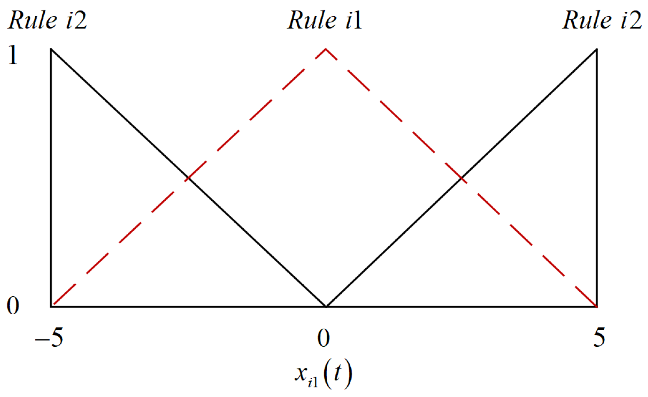
With the membership function (
Figure 1) and by solving the proposed conditions from Theorem 2, one can obtain the following controller gains with initial conditions
,
and performance matrices
,
and
.
For subsystem 1:
and
For subsystem 2:
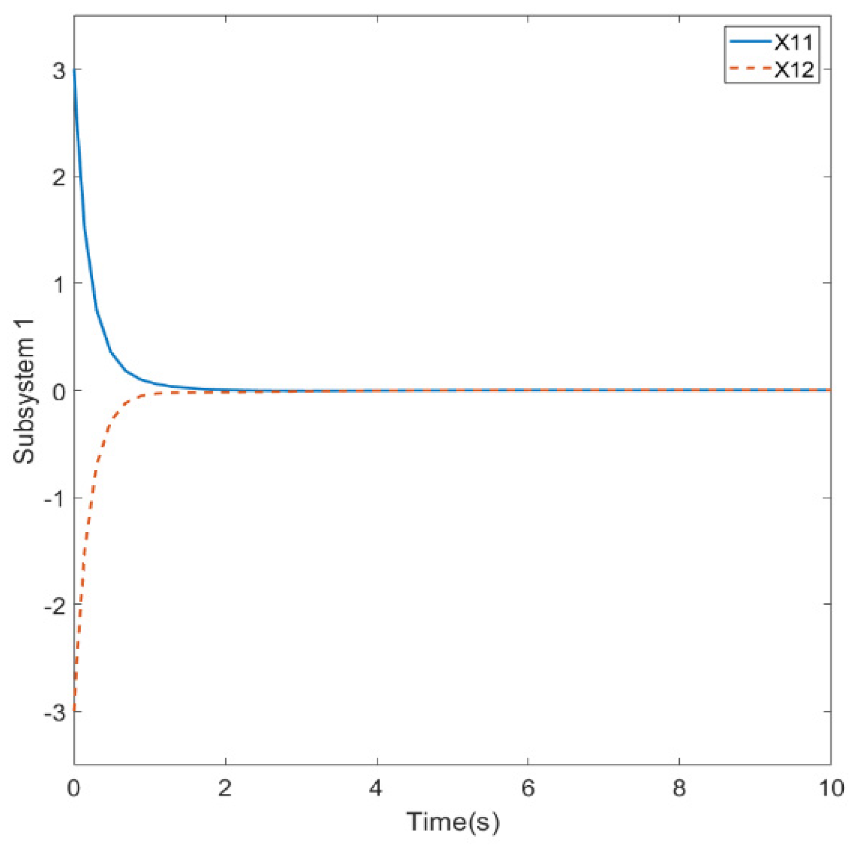
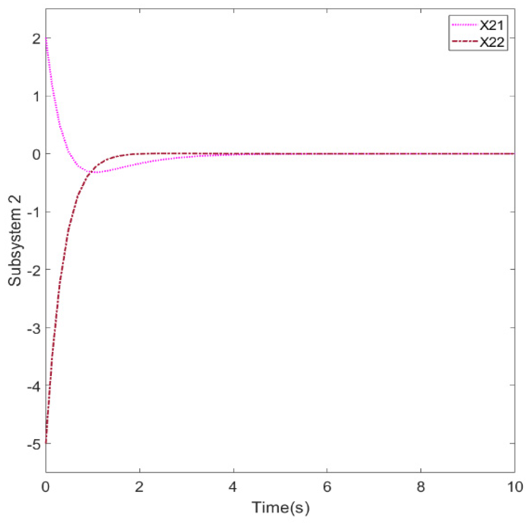
The state responses are shown in
Figure 2 and
Figure 3. In addition, the following scalar value is calculated to verify the CCC performance:
According to Definition 3, inequality (9) is satisfied with the above parameters, which implies that the CCC performance is well guaranteed under the minimization of output energy .
Based on the observations in
Figure 2 and
Figure 3, it is evident that the state trajectory gradually converges to zero over time. This convergence indicates that the controller gains proposed in Example 1 effectively stabilize the system. Furthermore, the system demonstrates quick and smooth stabilization under the CCC performance. This signifies that the proposed method delivers satisfactory performance.
Figure 2 and
Figure 3 validate the objective and effectively demonstrate the effectiveness of the proposed method.
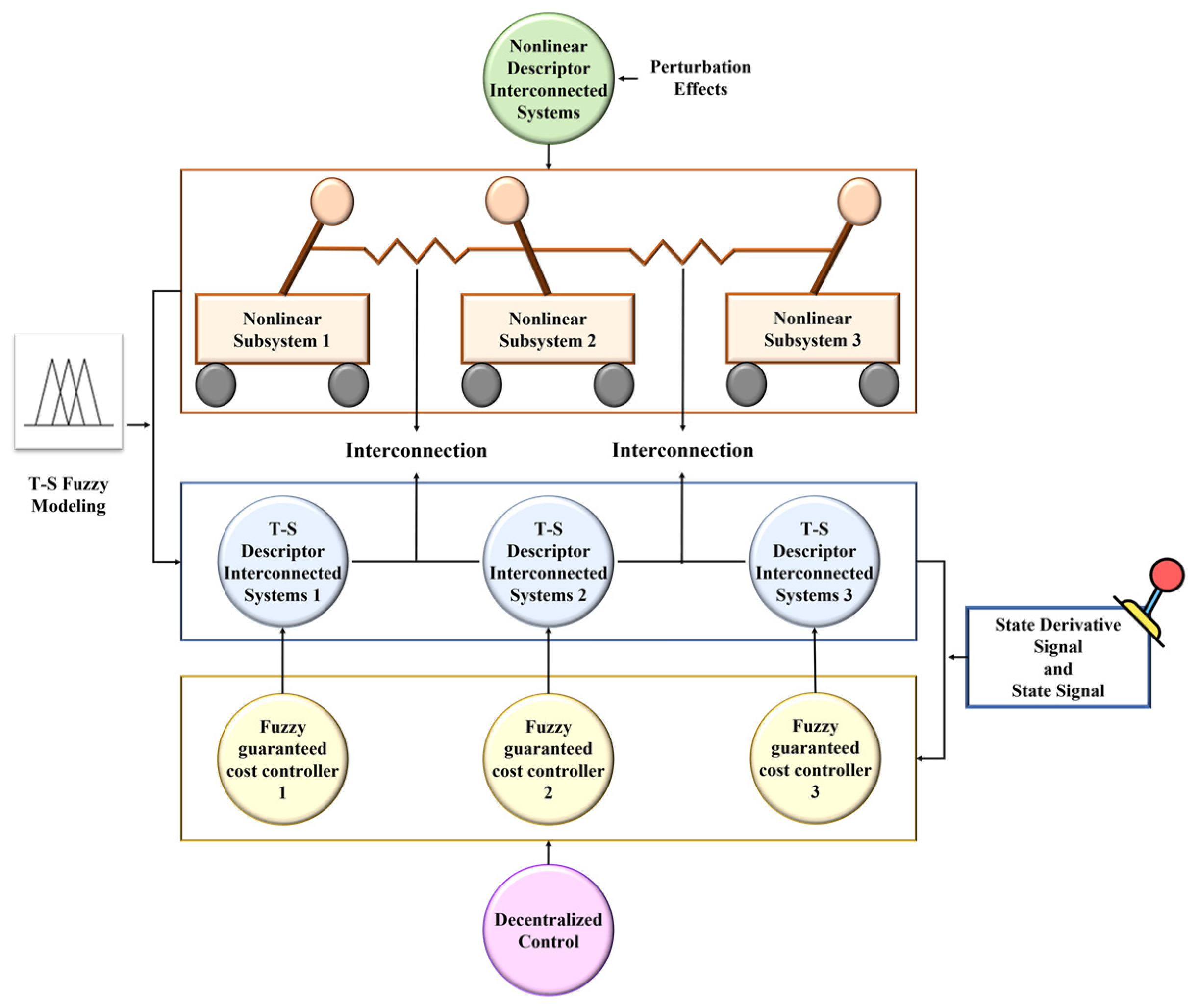
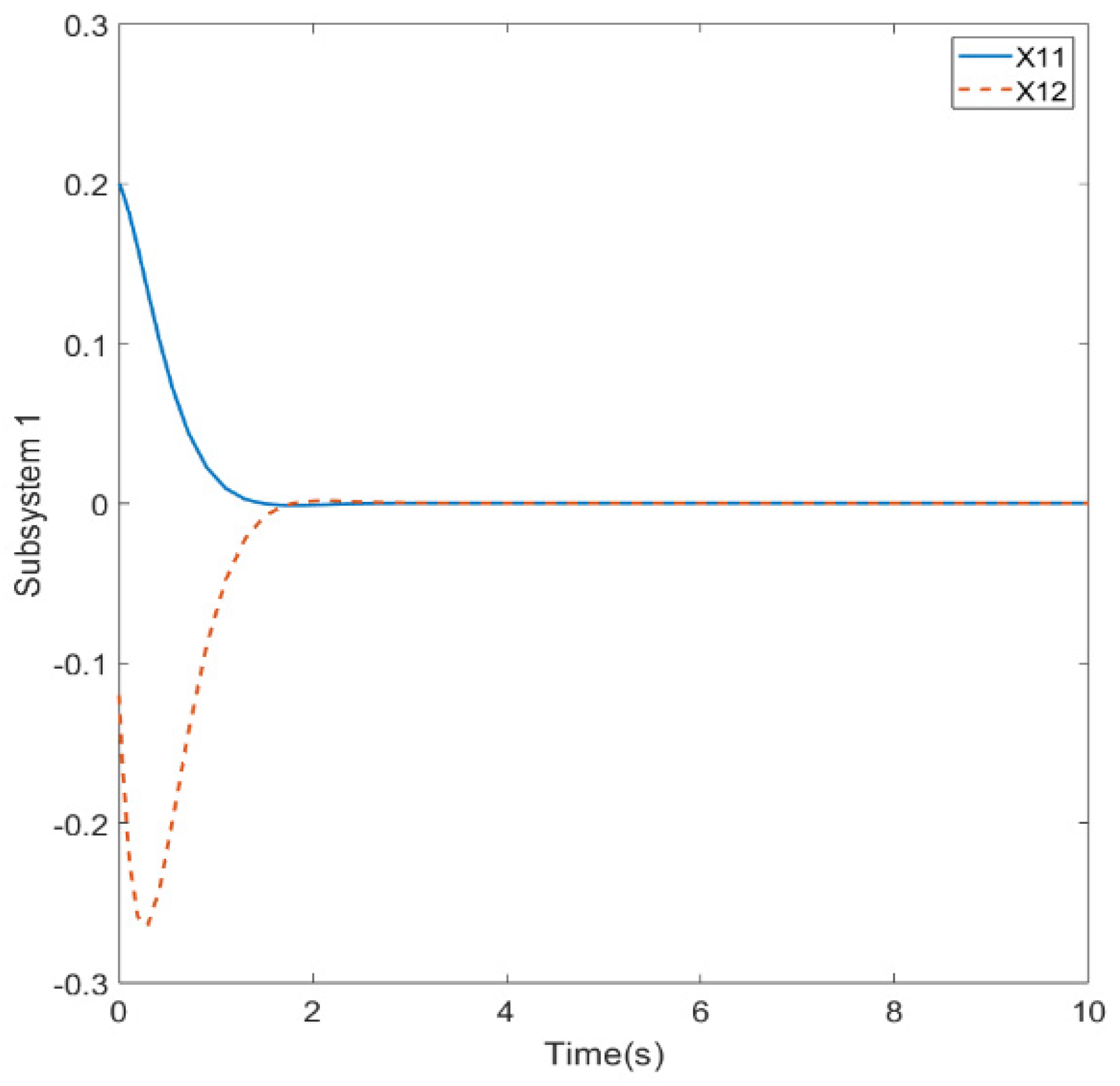
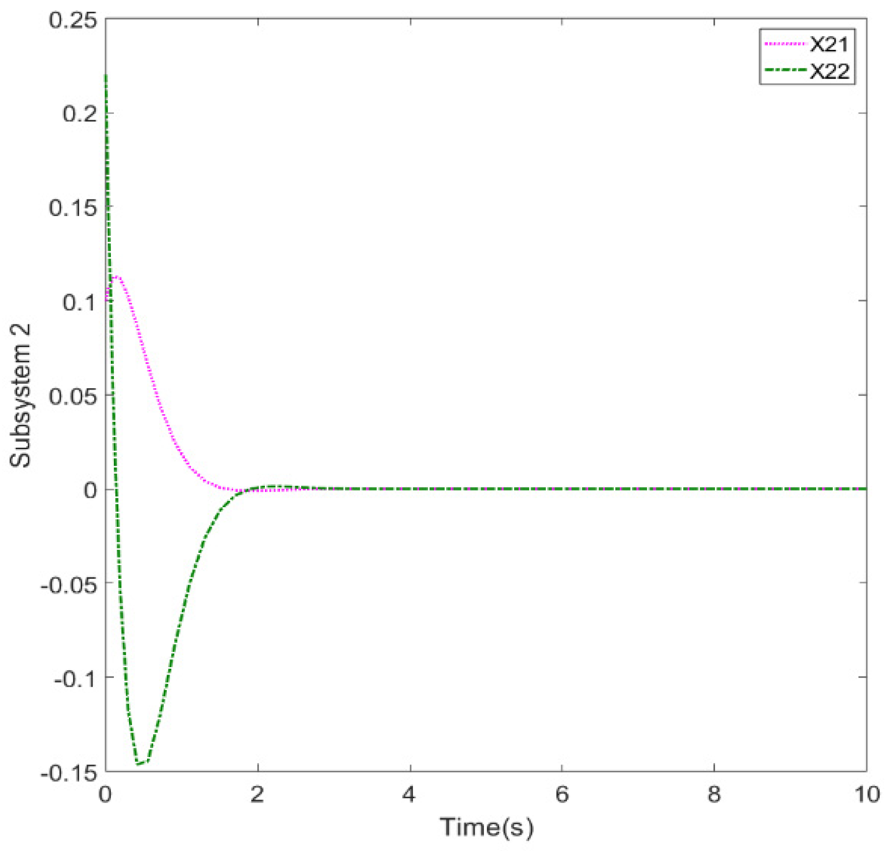
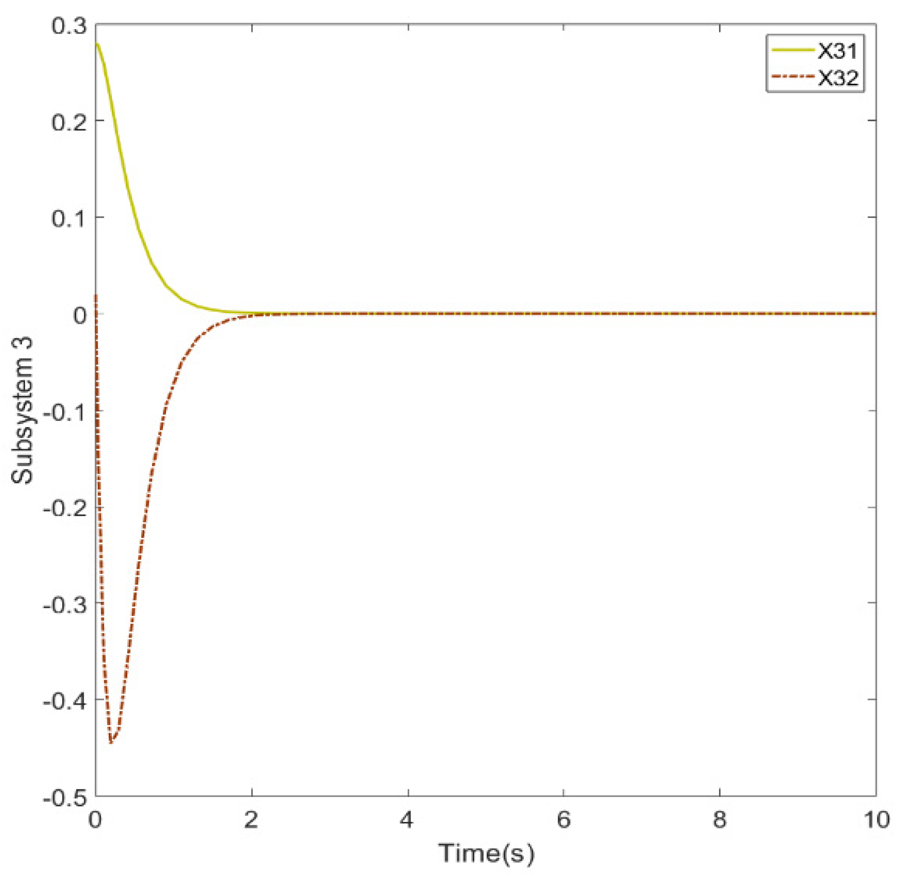
Example 2. The system under consideration is a nonlinear TIP system connected by two springs, as described in reference [20]. The nonlinear TIP system is a complex mechanical system that consists of multiple pendulums stacked on top of each other. Unlike a traditional pendulum that has a single mass attached to a fixed pivot, the TIP system incorporates additional masses and linkages, resulting in a highly nonlinear and dynamic behavior. In order to clearly demonstrate the proposed methodology, the control method for a nonlinear TIP system is presented in Figure 4.
where
represents the angular displacement of the pendulum
from the vertical reference;
denotes the torque input exerted by a servomotor at its base. All parameters have been provided in
Table 1.
By approximating the subsystems at
or
with the system form (6), the following system parameter can be obtained.
The uncertainties have been considered as
Considering the performance matrices , . Upon solving the conditions presented in Theorem 2, the feedback gains can be derived.
For subsystem 1:
For subsystem 2:
For subsystem 3:
With the initial conditions,
,
and
. The state responses are shown in
Figure 5,
Figure 6 and
Figure 7. According to the simulation results, all state responses converge to zero. That is to say, the DRCCFC proposed in this study can be effectively used in nonlinear DIS. Additionally, the CCC performance is satisfied for the tripled-inverted pendulum system with the following scalar values:
Stability: In a stable system, the state variables should converge to a steady state or equilibrium over time.
Transient Response: Evaluate how quickly the system reaches a steady state or desired condition. A faster transient response, where the state variables reach their desired values more rapidly, is often preferable. However, it is essential to balance speed with stability and avoid excessive overshoots or oscillations.
Overshoot and Damping: Assess whether the state response exhibits an overshoot, where the variables exceed their desired values before settling. Excessive overshoot can lead to instability, oscillations, or even system failure if it persists or grows uncontrollably.
Settling Time: Settling time is an important parameter, as it provides information about the system’s dynamic behavior and the speed at which it can achieve the desired state. A shorter settling time is generally better, as it indicates a faster system response and stability. However, too fast a settling time may cause overshoot in the system, so designing a controller with a faster settling time and reduced overshoot has always been a major problem in the field of control systems.
System Constraints: Consider any constraints or limitations specific to the system. For example, in control systems, there may be limitations in the control effort or actuator movements. A better state response adheres to these constraints while achieving the desired performance.
According to the simulation results, 0 represents the equilibrium point in the system. In the case of setting different initial state conditions, we can see that all states have converged to 0. This means that the designed controller can effectively control and stabilize T-S DIS. In addition, we can see that each state converges to 0 smoothly, which also means that the system does not have excessive overshoot when it is under control. Ultimately, CCC is a constraint that we choose to ensure that the total output energy of the system remains within predefined ranges or limits. From the calculated values of
and
, we can conclude that the inequality in (36) is satisfied, which also means that the simulation results meet the conditions of CCC. As a further explanation, in
Figure 2 and
Figure 3 and
Figure 5,
Figure 6,
Figure 7, since two different states are included, we designed different initial conditions to demonstrate the effectiveness of the controller. However, the initial evolution of the system will also have different results due to the different initial conditions, system matrices, and controller gains.
5. Conclusions
This paper studied the problem of CCC for nonlinear DIS with uncertainties. By constructing the QLF and FWF, sufficient stability conditions can be obtained based on the PDF control method and CCC function. In addition, the minimum value is also proposed to ensure that the system performance degradation is less than the upper bound. The proposed sufficient conditions for system stability can be cast into the LMI problems. Finally, we have provided two examples and simulation figures, which show the effectiveness and advantages of the proposed results. Based on the simulation results, it is evident that all states converge to 0, which indicates that the designed controller effectively regulates the T-S DIS and ensures its stability. Furthermore, the smooth convergence of each state to 0 signifies that the controlled system does not exhibit an excessive overshoot. This highlights the ability of the controller to maintain stable and controlled behavior without significant oscillations. In addition, the CCC is implemented as a constraint to ensure that the total output energy of the system remains within predefined limits or ranges. In fact, the system considered in this paper can be extended to the time-delay system, which could be the focus of our future work.


