1. Introduction
The traditional agricultural robot operations relying on manual control have low operation efficiency, high energy consumption, poor safety, and the quality of operation depends on the experience of agricultural machinery operators [
1]. Moreover, due to the increasing shortage of rural labor force, they are unable to meet the requirements of modern agricultural development. Therefore, the automatic driving technology has become the research focus in the intelligent planters, transplanters, harvesters, and other intelligent agricultural robots [
2,
3,
4,
5]. The farmland Complete Coverage Path Planning (CCPP), as one of the key technologies in autonomous agricultural robots [
6], aims at finding paths that cover all operating areas except obstacles. It has great significance for improving the operation efficiency of automatic driving agricultural robot, reducing the repeated work area and energy consumption [
7], ensuring the operation quality [
8], and promoting the development of precision agriculture [
9].
The CCPP methods mainly address the following problems [
10,
11,
12], (1) the entire work area must be traversed; (2) the static obstacles must be avoided; (3) the repeated work areas should be reduced as much as possible; and (4) the number of turns and U-turns should be minimized. The CCPP methods can be classified as grid-based method, cell decomposition-based method, neural network-based method, and heuristic algorithm-based method according to its implementation method.
The grid-based method, invented by W.E. Howden in 1968, divides the work area into several grids with equal size, and seeks the optimal path that has the minimum number of repeated grids and traverses all free grids. A high-resolution grid map representation-based online CCPP control algorithm [
13] was proposed to generate a smooth coverage path through Bezier curve approximation. The grid and HS (Harmony Search) algorithm-based path planner [
14] significantly reduced the number of trajectories turns. To solve the problem of path planning with a large number of grids, Ammar et al. [
15] improved the calculation times of the actual cost function. The grid-based methods have the advantages of simple implementation and easy planning; however, their computational complexity increases with the increasing number of grids.
The cell decomposition-based method firstly decomposes the work area into multiple sub-regions with simple shapes and without obstacles. Then the CCPP of each sub-region becomes a simple reciprocating movement, and can be implemented by seeking the optimal operation sequence of each sub-region. The boustrophedon-based decomposition method [
16] was presented to divide the region with excessive obstacle vertices. The decomposition method [
17] using different decomposition directions for different farmlands solved the problem that the traditional method can only be decomposed vertically. Although the cell decomposition methods have high efficiencies and significantly reduced the CCPP difficulty, the inappropriate connecting order of each sub-region can result in too many repeated paths.
The neural network-based CCPP method utilizes the self-learning ability and adaptability of neural network to improve the area coverage efficiency. A biologically inspired neural networks-based CCPP method [
18] was emerged to plan collision-free paths autonomously and in real time. The neural dynamics-based complete coverage navigation (CCN) algorithm [
19] can plan a shorter collision-free complete coverage path in an unknown environment. A complete coverage neural network (CCNN) [
20] was constructed, which can generate paths with smaller steering angles and fewer changes in navigation direction by the next optimal location decision strategy that combined with the driving direction. A feature-learning fully convolutional model [
21] was built to solve the crop row-based CCPP problem. The neural network brings new ideas to solve the CCPP problem, whereas it has a lower planning success rate when the data are insufficient, and its loss function has less robustness.
The heuristic algorithms-based CCPP method utilizes the heuristic factors to reduce the complexity of the search problem, thereby improving the efficiency of searching the optimal paths. The bacterial foraging method [
22] for robot path planning is proposed to plan the best collision-free path between the starting point and the target point, and it can plan stable and reliable trajectories in complex environments. A new mix-opt operator for simulated annealing algorithm [
23] was proposed to accelerate the convergence speed of heuristic optimization. The CCPP method combining the genetic algorithm and TSP (Travel Quotient Problem) [
24] can find the coverage path that has the shortest travel distance and grid coverage time. A novel integrated virus evolution heuristic algorithm [
25] that satisfies the trade-off between multiple objectives is proposed for intelligent toolpath optimization, which can obtain the direct output of the global optimized toolpath, and has very important industrial strategic capabilities. The Non-Dominated Sorting Genetic Algorithm (NSGA-III) [
26] takes the maximum volume of pesticide tanks into consideration, and can seek out the coverage path with minimum travel distance and routing angle. It can solve the CCPP problem of multi-agricultural mobile robot. A self-reconfigurable autonomous robot [
27] that can enter the narrow space was created, and can conduct the CCPP by optimizing the order of traveler sequences. Focusing on the irregular fields with a single entrance, a search space with virtual obstacles [
28] was generated that can use the A* algorithm to determine a curved path for returning to the entrance after completed an agricultural task. The heuristic algorithm-based CCPP methods have the advantages of easy implementation, high capability of seeking the optimum solution, and fair extensibility [
29].
Many scholars have done in-depth research on complete coverage path planning technology, which is of significance for the further research and application of this technology in intelligent agricultural robots. Each path planning method mentioned above has its own advantages and limitations, and their differences are summarized in
Table 1, a comparison table of complete coverage path planning methods. Among them, the genetic algorithm has the advantages of high optimization ability and parallel ability, easy coding, and combination with other algorithms, and can effectively solve multi-objective optimization problems. Hence, this paper uses the improved genetic algorithm to solve the complete coverage path planning problem.
The grid-based, cell decomposition-based, and neural network-based CCPP methods have obtained many research achievements; however, they still have some problems such as high path repetition rate, low planning efficiency, and poor robustness when coping with complex working scenarios. Therefore, the heuristic-based CCPP method with good stability and strong global optimization-seeking ability was used in this paper to deal with the complex farming scenarios that have irregular boundaries and obstacles. Nonetheless, the adopted classical heuristic genetic algorithm is prone to the local optimal solution in the actual planning. Thus, an improved genetic algorithm-based [
30] CCPP method was proposed in this paper to improve the global optimization-seeking ability and environmental adaptability of the classical genetic algorithm in complex environments. The proposed method innovatively extends the traditional genetic algorithm’s chromosomes and single-point mutation into chromosome pairs and multi-point mutation, which can reduce the repeated area and the number of turns and U-turns. The proposed CCPP method can guide the autonomous agricultural robot to achieve efficient cultivation especially in complex field environments. The main contributions of this paper are as follows, (1) extends the chromosomes to chromosome pairs that contains a chromosome for genetic evolution and a chromosome for fitness calculation, which increases the efficiency and operational effectiveness of CCPP; (2) proposes a multi-point mutation method to break the genetic sequence of the parent chromosomes as much as possible, which improves the global optimization-seeking ability in a complex environment; and (3) establishes a multi-objective fitness function that takes account of the repeated operation area, the number of turns and U-turns, which reduces the overall energy consumption.
2. Materials and Methods
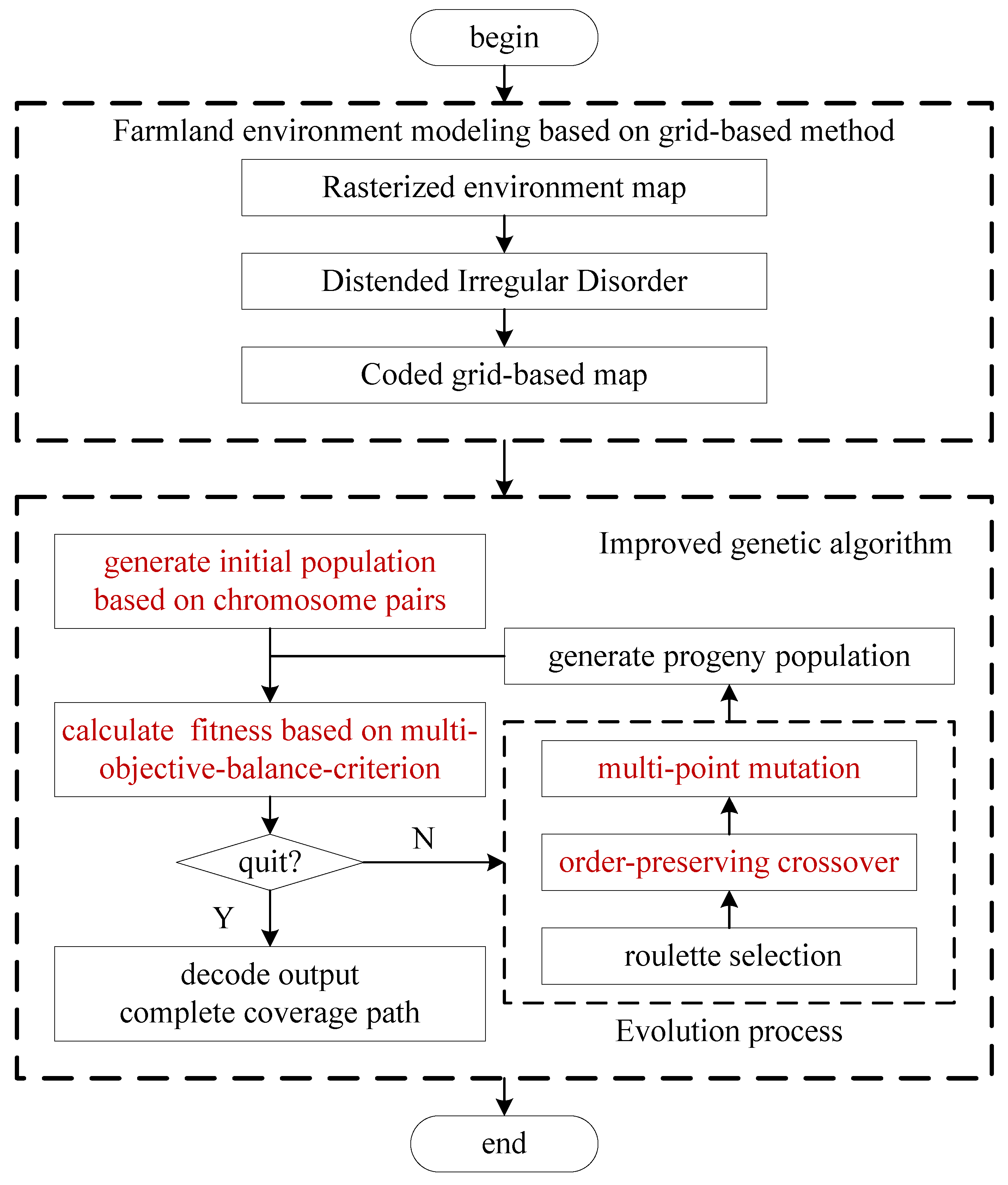
The proposed improved-genetic-algorithm-based CCPP method consists of two parts, (1) the field environment map modeling and (2) the improved genetic algorithm for CCPP. As shown in
Figure 1, the field environment map modeling includes three modules, (1) environment map rasterization, which divides the environment map into grids with equal size; (2) irregular object dilation, which dilates the irregular-sized obstacles and irregular-shaped fields into regular grids; and (3) grid map coding, which adopts the sequential notation method to code the grids. The improved genetic algorithm for CCPP includes six modules, (1) chromosome-pairs-based initial population generation, which generates the initial Q chromosome pairs; (2) multi-objective-balance-criterion-based chromosome fitness calculation, which is used for algorithm iterative update; (3) elitist-strategy-based roulette selection, which selects a limited number of chromosomes with the best fitness values to pass to the next generation population; (4) order-preserving crossover, which aims to inherit the excellent genes of the parent chromosomes and ensure the stability of the population; (5) multi-points mutation, which introduces diversity in the genetic population and expands the search space; and (6) optimal complete coverage path (OCCP) output, which decodes and outputs the OCCP when the termination condition is satisfied.
2.1. Field Environment Map Modeling Based on Grid Method
The field environment mapping is the foundation of CCPP for self-driving agricultural robots. The grid map can accurately represent the environmental information, and is easy to maintain, store, and be used for solving the CCPP problem. Therefore, the grid map construction method was adopted in this paper for representing the field boundaries, free space, and obstacles in an real field. The grid-map-based field environment modeling includes (1) environment map rasterization, (2) irregular object dilation, and (3) grid map coding, which are detailed as follows.
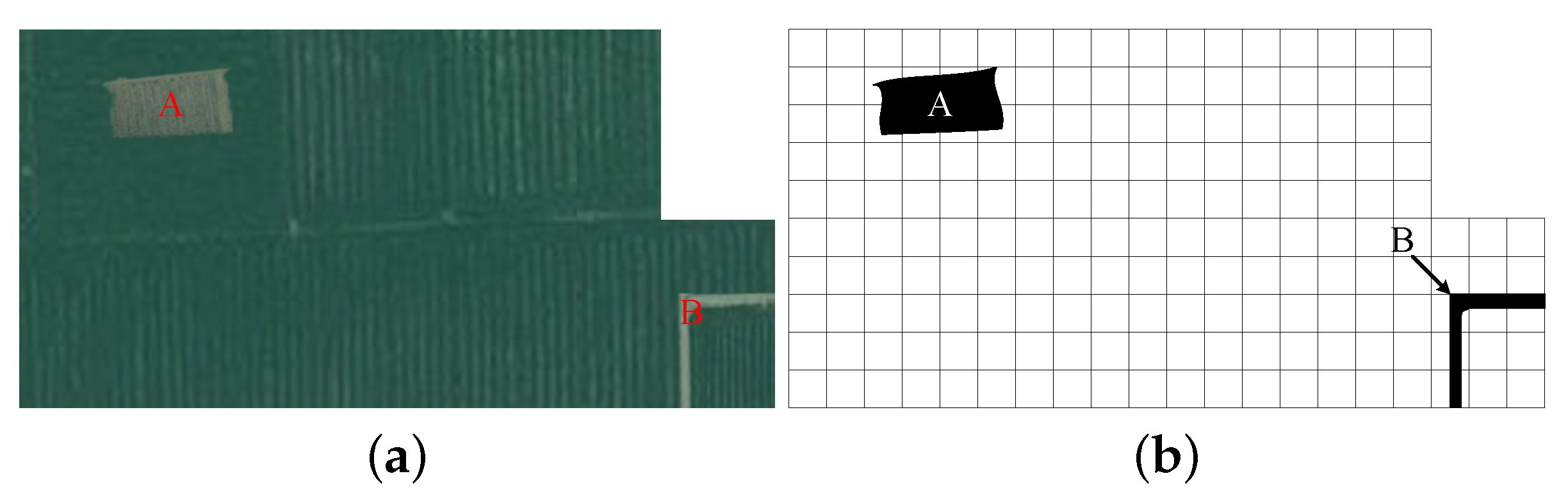
2.1.1. Rasterization of the Environment Map
The environment map rasterization is the first task for creating the environment grid map, which divides the environment map into grids with equal area. As shown in
Figure 2, the field map shown in
Figure 2a is rasterized into the grid map shown in
Figure 2b. The grid size can be determined by the size and the operation width of the autonomous driving agricultural robot. In addition, the obstacles are projected to the grid map, e.g., the obstacle A and B in
Figure 2.
2.1.2. Irregular Grid Expansion
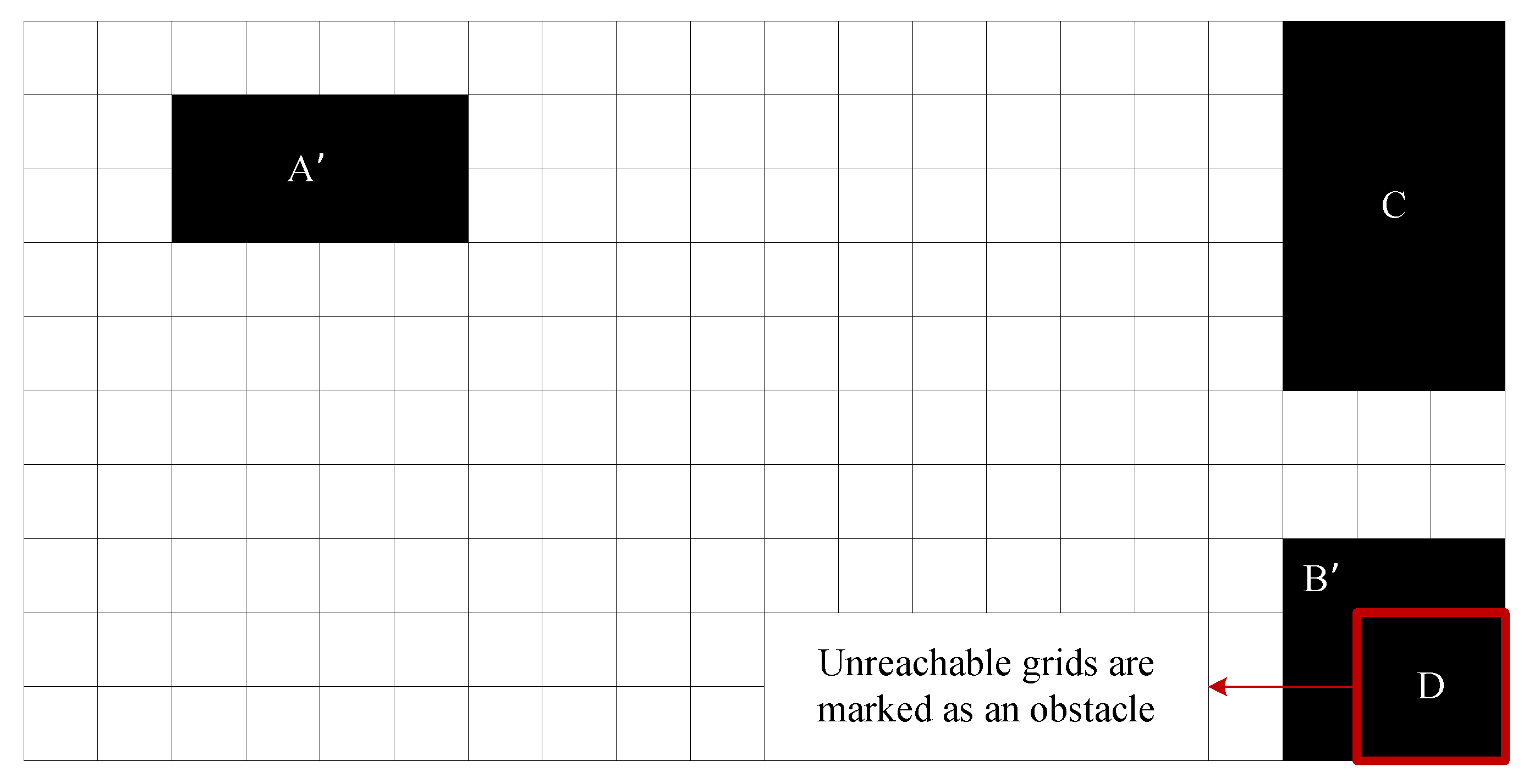
When the field has an irregular shape or some static obstacles existed in the field, the rasterized field map needs to be dilated into a regular-shaped map, and the irregular-shaped obstacles into regular-shaped obstacles. This will help to determine whether a grid is reachable. For example, the grid map shown in
Figure 2b was dilated to the grid map shown in
Figure 3. Area C in
Figure 3 was added to regularize the grid map and the irregular-shaped obstacle A in
Figure 2b were dilated into the regular-shaped obstacle A’ in
Figure 3. In addition, because the area D in
Figure 3 surrounded by L-shaped obstacle B in
Figure 2b is an unreachable, the L-shaped obstacle B in
Figure 2b should be dilated into the rectangular obstacle B’ in
Figure 3.
2.1.3. Grid-Based Map Coding
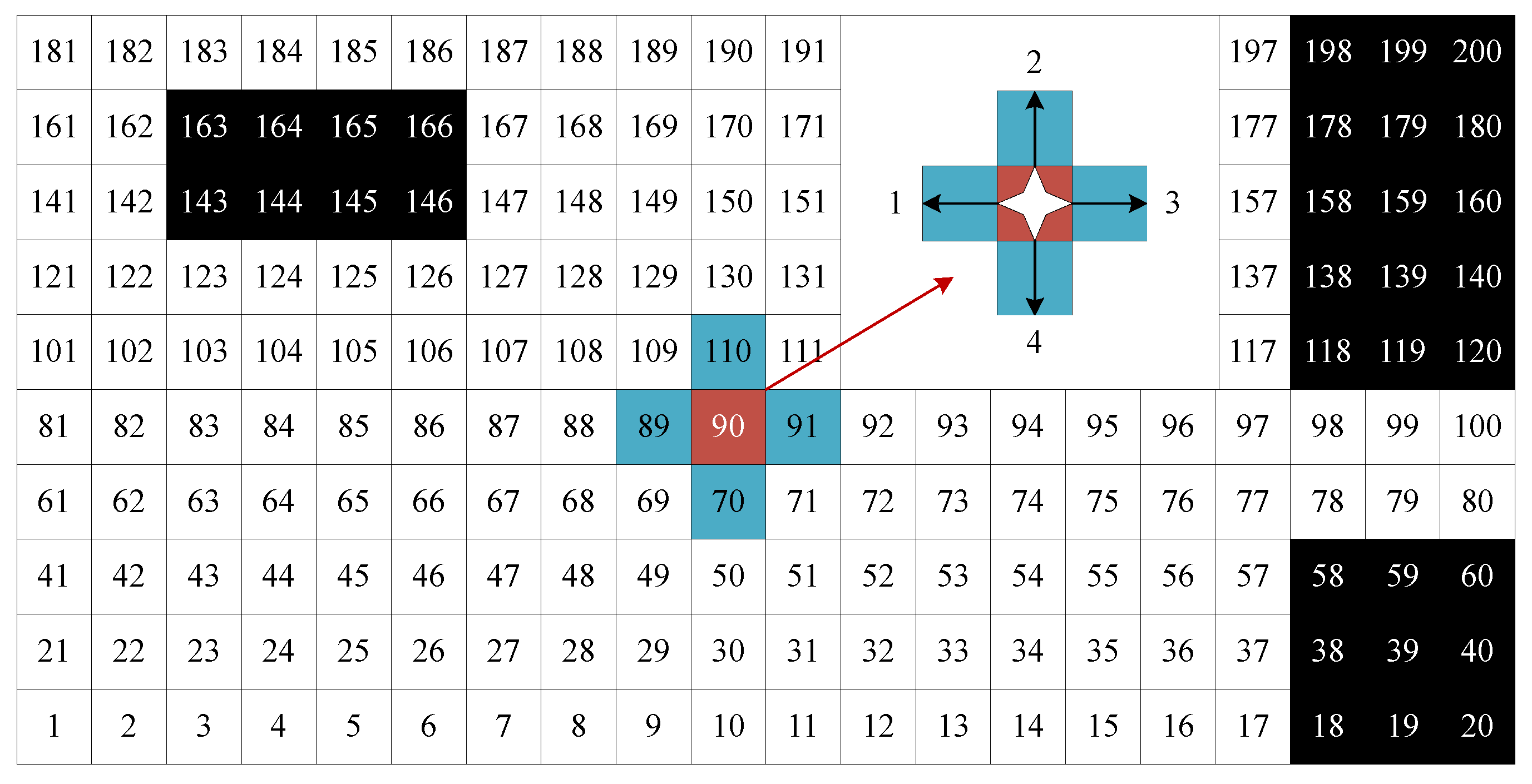
For the convenience of solving the CCPP problem and presenting the final planned path, the sequential notation method was adopted to encode the map grids in this paper. As shown in
Figure 4, the grid map was encoded, starting from the bottom left grid, and each grid is sequentially marked as the unique number in the order of left to right and bottom to top. Meanwhile, the black occupied grid (e.g., 18–20, 143–146, 118–120) was labeled as “1”, and the white free grid (e.g., 61–117) as “0”, for identifying the properties of different grids. Therefore, each grid is represented as
, where
is the unique number of the grid, and
is the grid property. When the CCPP method searches for the OCPP, the 4-neighbor searching method was employed for reducing the CCPP searching spaces. For example, if the autonomous driving agricultural robot is at the position <90,0> in
Figure 4, its 4-neighbor were <89,0>, <91,0>, <70,0>, and <110,0>, namely the one-step reachable search domain of the grid <90,0>. For ease of calculating the number of turns and U-turns (see
Section 2.2.2), the left movement (e.g., from <90,0> to <89,0> in
Figure 4 is marked as 1, up movement (e.g., from <90,0> to <110,0> in
Figure 4 as 2, right movement (e.g., from <90,0> to <91,0> in
Figure 4 as 3 and down movement (e.g., from <90,0> to <70,0> in
Figure 4 as 4.
2.2. Field CCPP Based on Improved Genetic Algorithm
Since the traditional-genetic-algorithm-based CCPP method, when coping with the irregular-shaped field, and other complex field with obstacles, is prone to the problems, such as more repeated work area, more turns or U-turns, and falling into local optimum, an improved-genetic-algorithm-based CCPP method was proposed in this paper. This method innovatively proposes the chromosome pairs and multi-points mutation to improve its global optimization ability in complex environments, and the multi-objective (i.e., the repeated work area, the number of turns and U-turns)-balance-criterion-based chromosome fitness function to reduce the number of turns and U-turns under the premise of less repeated work area. The improved genetic algorithm includes (1) chromosome-pair-based initial population generation, (2) multi-objective-balance-criterion-based chromosome fitness calculation, (3) elitist-strategy-based roulette selection, (4) order-preserving crossover, (5) multi-points mutation, and (6) OCCP output, which are detailed as follows. Furthermore, the algorithm needs to meet the following conditions, (1) the shape of the grid map is a regular rectangle; (2) the number of grids in the grid map is limited; (3) the feasible area and obstacle area of the known grid map; and (4) does not consider the mileage constraints of agricultural robots. At the end of the algorithm run, the output optimal chromosome is decoded into the optimal path order.
2.2.1. Initial Population Generation Based on Chromosome Pairs
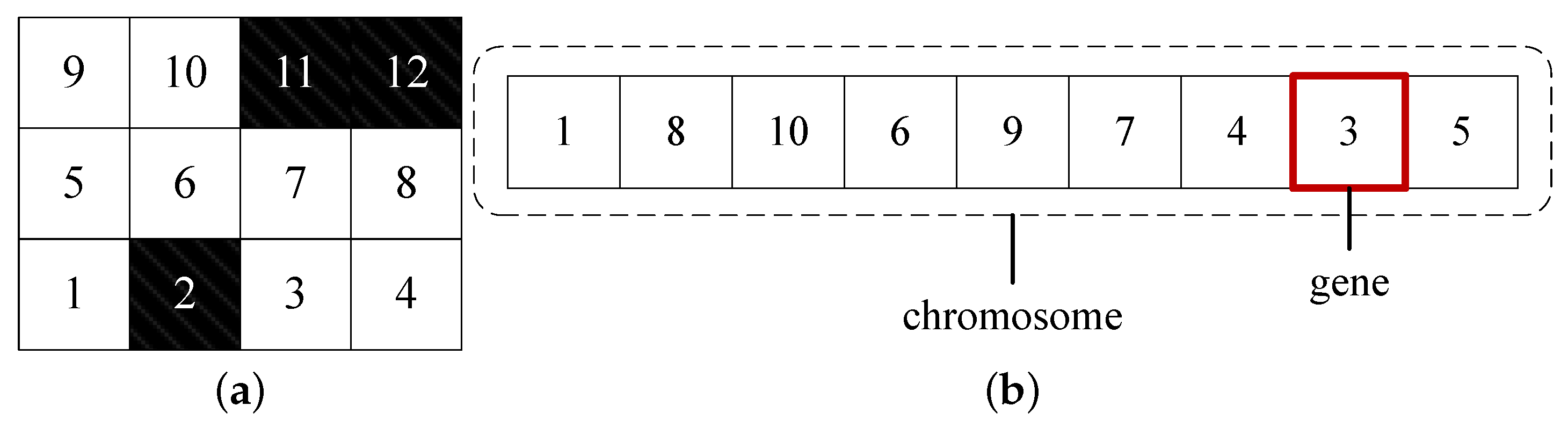
The CCPP aims to traverse all the free grids, and the traversed grid order is the planned complete coverage path. To describe the encoding scheme with a minimum encoding character set, a decimal encoding is adopted in this paper. Each chromosome represents a feasible solution, i.e., a field complete coverage path, where the grid in set
presents at least once, while the grid in set
is absent. For example, an initial chromosome
in
Figure 5b corresponding to the encoded grid map in
Figure 5a, can be randomly generated.
The traditional genetic algorithm randomly generates Q chromosomes as the initial population. However, for the CCPP problem, the randomly generated initial population is prone to a large number of invalid chromosomes. For example, the chromosome shown in
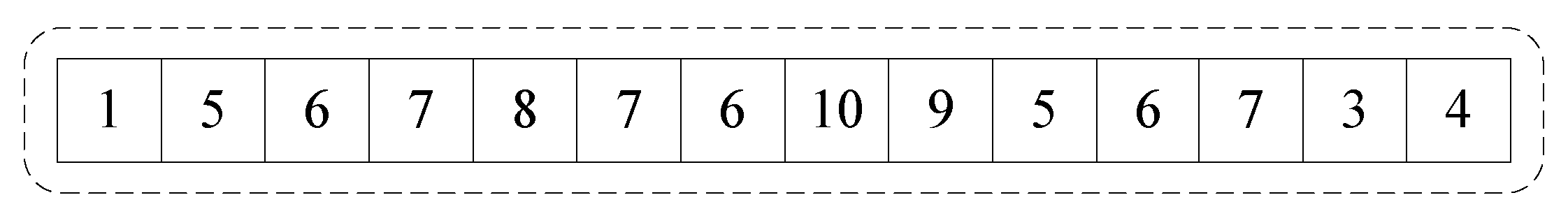
Figure 5b is an invalid chromosome since the 4-neighbor relationship between gene 1 and gene 8 is not satisfied, i.e., gene 8 is not in the one-step reachable search domain of gene 1. In other words, the autonomous driving agricultural robot cannot directly move from grid 1 to grid 8. Therefore, the randomly generated chromosome is adjusted in this paper to obtain the chromosome (as shown in
Figure 6) that the adjacent genes satisfied the 4-neighbor relationship.
The proposed adjustment method of the chromosome is described as follows:
- (1)
If two adjacent genes satisfy the 4-neighbor relationship, i.e., the adjacent genes are one-step reachable, no adjustment is required.
- (2)
If two adjacent genes do not satisfy the 4-neighbor relationship, the gene sequence where the adjacent genes satisfy the 4-neighbor relationship with the shortest path was inserted between the two genes. If the inserted gene appears in the subsequent gene sequence of the chromosome, the repeated genes appeared in the subsequent gene sequence will be deleted. The Floyd’s algorithm [
31] was used in this paper to find the gene sequence with the shortest path that should be inserted.
- (3)
Starting from the first gene of the chromosome, step (1) and step (2) were repeated until all the genes of the chromosome were traversed. Thus, the valid chromosome where all the adjacent genes satisfy the 4-neighbor relationship will be generated.
For example, the process of adjusting the invalid chromosome shown in
Figure 5b to the valid chromosome shown in
Figure 6 is as follows:
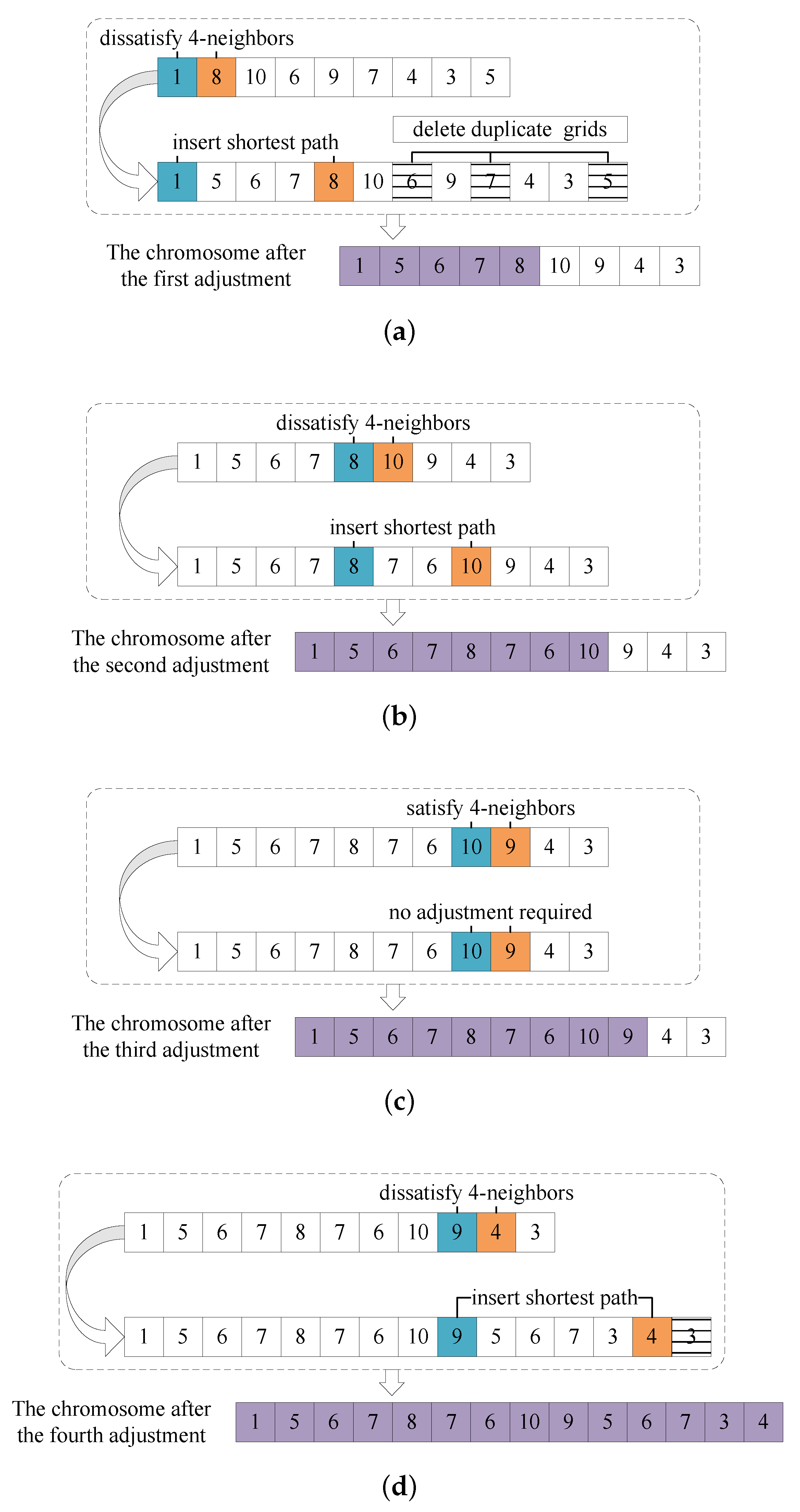
- (1)
As shown in
Figure 7a, starting from the first gene, the shortest path 5-6-7 obtained by the Floyd’s algorithm was inserted between gene 1 and gene 8 since gene 1 and gene 8 do not satisfy the 4-neighbor relationship. In addition, the genes 5, 6, and 7 appeared in the subsequent gene sequence of the chromosome are deleted, and the adjusted chromosome 1-5-6-7-8-10-9-4-3 will be obtained.
- (2)
As shown in
Figure 7b, next traversing the gene 8, the shortest path 7-6 obtained by the Floyd’s algorithm was inserted between gene 8 and gene 10 since gene 8 and gene 10 do not satisfy the 4-neighbor relationship. Because gene 7 and gene 6 was absent in the subsequent gene sequence, the chromosome 1-5-6-7-8-7-6-10-9-4-3 can be obtained without gene deletion operation.
- (3)
As shown in
Figure 7c, continually traversing the next gene 10, because gene 10 and gene 9 satisfy the 4-neighbor relationship, no adjustment was done. Then traversing the next gene 9, as shown in
Figure 7d, the shortest path 5-6-7-3 was inserted similarly as (1) between gene 9 and gene 4, and the repeated gene 3 was deleted. Since gene 4 was the last gene of the chromosome, the chromosome adjustment was finished. Finally, the adjusted valid chromosome is 1-5-6-7-8-7-6-10-9-5-6-7-3-4 where all free grids appeared at least once and all the adjacent genes satisfy the 4-neighbor relationship.
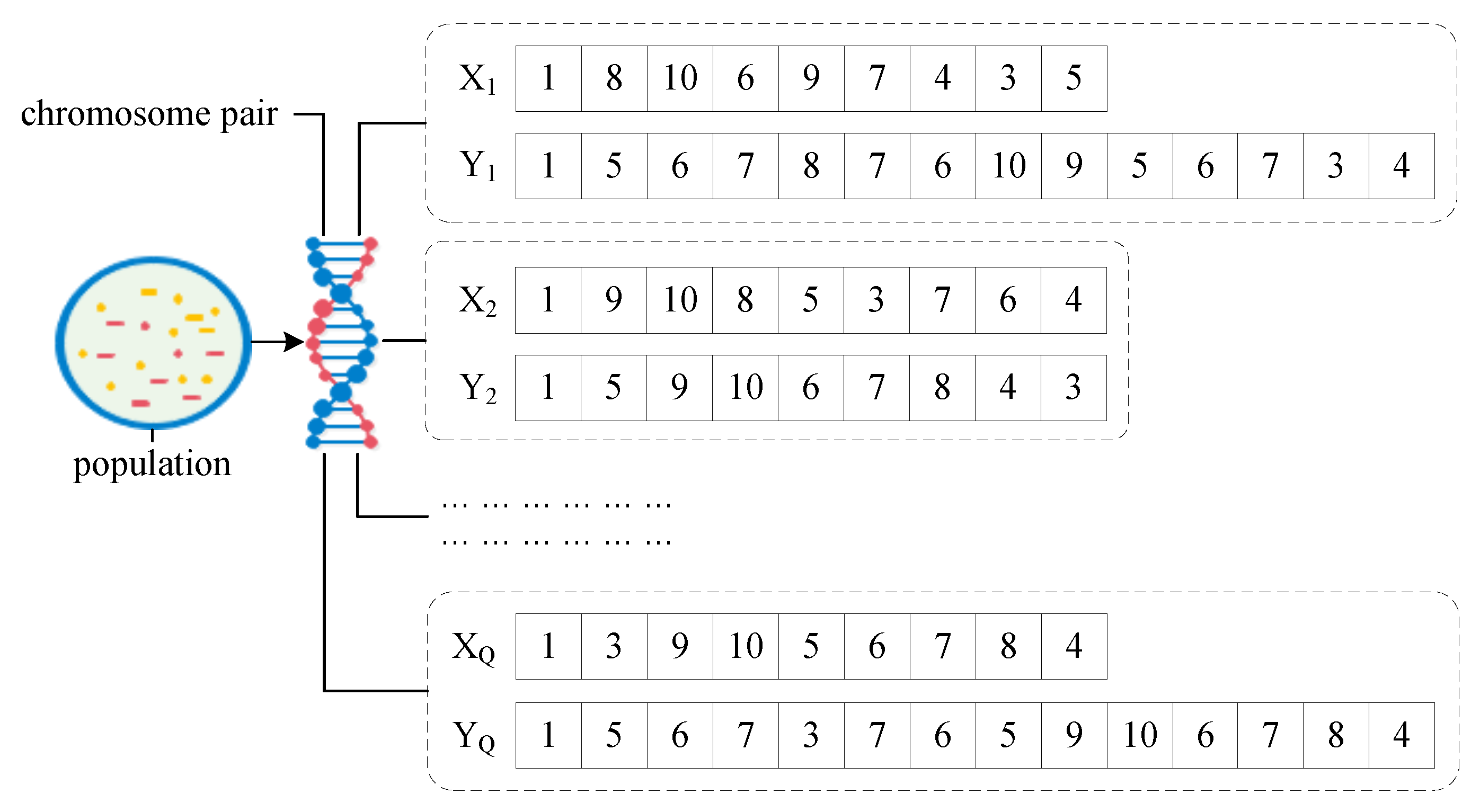
As shown in
Figure 7, the chromosome pair was generated by combining the chromosome
= 1-8-10-6-9-7-4-3-5 and the adjusted valid chromosome
= 1-5-6-7-8-7-6-10-9-5-6-7-3-4. Thus, the initial population
show in
Figure 8 can be obtained by combing the Q chromosomes
randomly generated by the traditional genetic algorithm and its adjusted valid chromosomes
. The chromosome
X in the initial population has the same number of genes, and was used for selection, crossover, mutation, and other evolutionary operations. The chromosome
Y in the initial population may have different number of genes, and was used for chromosome fitness calculation. Moreover, the chromosome
Y represents a complete coverage path that an autonomous driving agricultural robot can travel in the real farming operation.
2.2.2. Fitness Calculation Based on Multi-Objective Equalization Criterion
The fitness function is the basis of the genetic algorithm iteration, and is the key factor of generating optimal solution and algorithm convergence. Because the turns and U-turns will produce a deceleration–reacceleration process, and increase the energy consumption of agricultural robot, the main objective of CCPP is to reduce the number of turns and U-turns as much as possible while covering all the free grids. However, in practical farming operation, the number of turns or U-turns was inevitably increased to reduce the repeated work area, or the repeated work area was increased to reduce the number of turns or U-turns. Therefore, to balance the cost of the number of turns, the number of U-turns, and the repeated work area [
32], a multi-objective-balance-criterion-based fitness function was proposed in this paper, which was defined as follows
where
represents the fitness value of the i-th chromosome;
,
and
represent the weight of the repeated work area, the weight of the number of turns and the weight of the number of U-turns, respectively, which were defined in (
2) to (
7); and
,
and
represent the repeated work area, the number of turns and the number of U-turns, which were defined in (
11) to (
15).
The initial weight of
,
, and
are set to 0.3, 0.2, and 0.5, then the weight adaptive mechanism was used to balance the three objectives with the following formula,
where
,
and
represent the weights of the i-th chromosome in current population;
,
and
represent the weight of the i-th chromosome in parent population;
,
and
represent the repeated work area, the number of turns and the number of U-turns of the i-th chromosome in current population, respectively; and
,
and
represent the average of the repeated work area, the number of turns and the number of U-turns of all chromosomes in parent population, respectively, which were defined in (
8) to (
10).
The repeated work area
, the number of turns
and the number of U-turns
of the i-th chromosome were calculated according to the Y chromosome, which are defined as follows:
where
represents the length of the chromosome
;
represents the length of the chromosome after removing its repeated genes; % represents the mod operation;
represents the moving direction of the autonomous driving agricultural robot at the grid
; and
,
represent whether the autonomous driving agricultural robot has the turn and U-turn action at the grid
, respectively.
2.2.3. Roulette Selection Operation Based on Elite Strategy
The elitist-strategy-based roulette selection was adopted in this paper to make the optimal k elite chromosomes in the parent population be inherited to the offspring population. In addition, the remaining chromosomes in the parent population are selected by the roulette algorithm until the desired number of offspring chromosomes are satisfied. Thus, each chromosome has the probability that proportional to its fitness value to enter the offspring generation, and the chromosomes both with low fitness value and high fitness value are selected. This will make the population have the diversity, and make the algorithm avoid falling into a local optimum [
33]. The probability
of a chromosome being selected in the population is defined as follows:
where
i represents the
i-th chromosome;
represents the fitness value of the
i-th chromosome (as shown in (
1)); and Q is the total number of chromosome in the population.
2.2.4. Crossover Operation Based on Order-Preserving Method
Crossover is one of the important steps in the evolution of genetic algorithm, which is analogous to reproduction and biological crossover. In crossover operation, more than one parent is selected with a high probability and one or more off-springs are produced using the genetic material of the parents, which will enhance the algorithm’s optimization ability. The order-preserving crossover method was used in this paper, which was detailed as follows. Firstly, two chromosomes, A and B, were randomly selected for crossover in the parent population. Then a crossover point of chromosome A was randomly determined, and the genes behind this point in chromosome A were deleted. Next the genes at the front of the crossover point in chromosome A were deleted from chromosome B. Finally, the remaining genes in chromosome B were added behind the crossover point of chromosome A, and a new chromosome C will be obtained. The crossover probability is generally between 0.5 and 1. The crossover not only ensures that the off-spring chromosome contains all the free grids, but also has the characteristics of the parent chromosome.
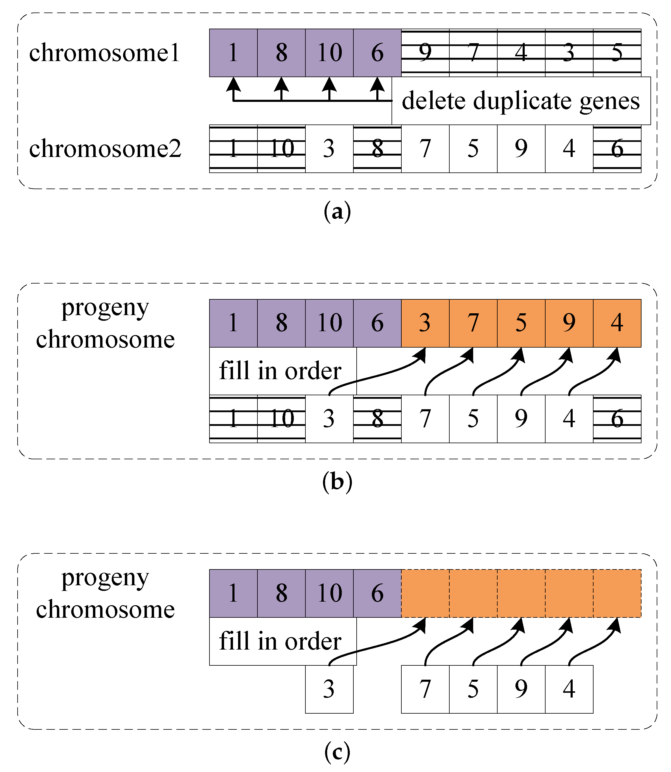
For example, the order-preserving crossover operation are shown in
Figure 9. Firstly, as shown in
Figure 9a, the crossover point was randomly determined, i.e., gene 6 in chromosome 1 and gene 8 in chromosome 2. Then, as shown in
Figure 9b, gene 1, 8, and 10 (appeared before the crossover point in chromosome 1) were deleted in chromosome 2, and the genes (i.e., gene 9, 7, 4, 3, and 5) behind the crossover point in chromosome 1 were deleted. Finally, as shown in
Figure 9c, the remaining gene sequence 3-7-5-9-4 was added in order behind the crossover point of chromosome 1, and the off-spring chromosome 1-8-10-6-9-7-4-3-5 can be obtained. Similarly, the off-spring chromosome generated by the order-preserving crossover operation also should be adjusted by the method in
Section 2.2.1 to calculate its fitness value.
2.2.5. Mutation Operation Based on Multi-Points Method
Mutation is one of the important steps in the evolution of genetic algorithm. Mutation can be defined as a small random tweak in the chromosome to obtain a new solution, which can maintain and introduce diversity in the genetic population. It is usually applied with a low probability since the GA will become reduced to a random search if the probability is very high. Mutation is essential to the convergence of the genetic algorithm. A novel mutation operation, namely multi-points mutation, was proposed in this paper to improve the ability to search for the optimal solution, which is described as follows. Firstly, the number (m) of gene pairs for mutation was randomly determined, and the gene positions of the m pairs for mutation were also randomly determined. Then, the two genes in each pair of mutation points were exchanged, and, finally, a new chromosome can be obtained. The mutation probability is generally between and . The multi-points mutation can significantly destroy the gene sequence of the parent while ensures that the off-spring chromosome contains all the free grids, which helps the algorithm avoid to fall in local optimum.
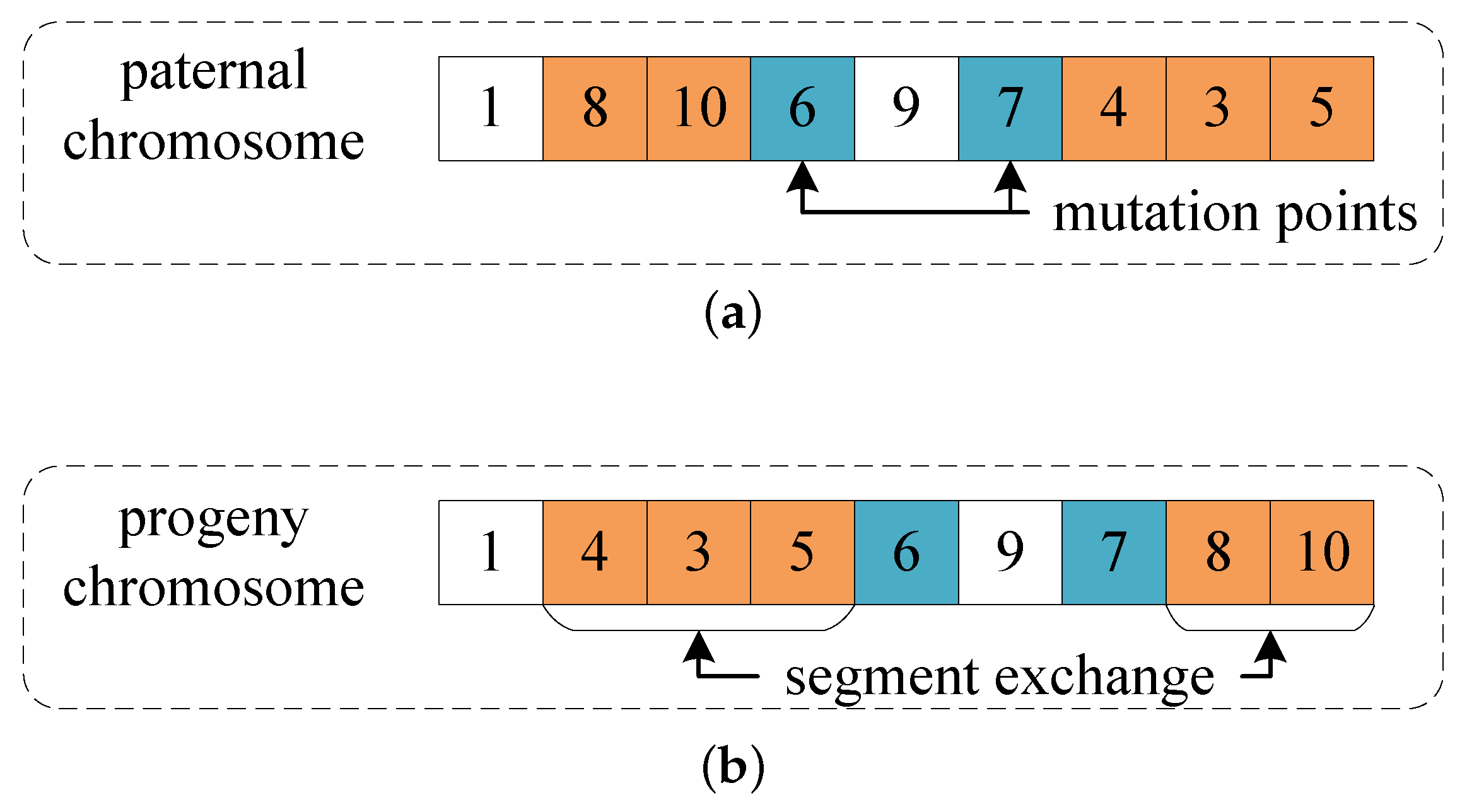
For example, the multi-points mutation operation was shown in
Figure 10. Firstly, two mutation points were randomly identified, e.g., gene 6 and gene 7 in
Figure 10a. Then keeping the gene 1 unchanged, the chromosome segments before gene 6 and after gene 7 were interchanged, as shown in
Figure 10b. Finally, the progeny chromosome 1-4-3-5-6-7-8-10 after mutation was obtained. Similarly, the progeny chromosome generated by the multi-points mutation operation also should be adjusted by the method in
Section 2.2.1 to calculate its fitness value.
2.3. Outputting the Optimal Complete Coverage Path
Genetic algorithm usually has two conditions of termination, (1) setting the maximum number of generations, and (2) the fitness tends to stable. The former was that when the maximum number of iterations was reached, the algorithm was terminated and output the optimal solution. The latter was that when the fitness value of the optimal solution was less than the pre-set threshold or the fitness value was unchanged for many iterations (e.g., M times, which also was preset), the algorithm can be terminated and output the optimal solution. Both conditions were adopted in this paper, the maximum number of iterations was set, and if the condition (2) was satisfied, the algorithm can be terminated early; otherwise, the algorithm will be terminated until the maximum number of iterations was reached.
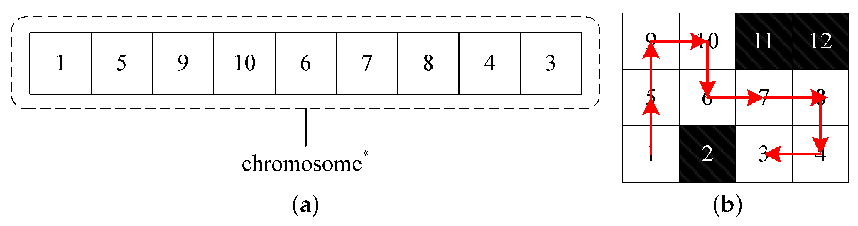
When the algorithm was terminated, the OCCP, i.e., the adjusted chromosome
Y in the chromosome pair can be acquired. For example, if the optimal solution was the optimal adjusted chromosome
shown in
Figure 11a, its corresponding OCCP was shown in
Figure 11b.
3. Results and Discussion
Heuristic algorithm is a basic method to solve optimization problems [
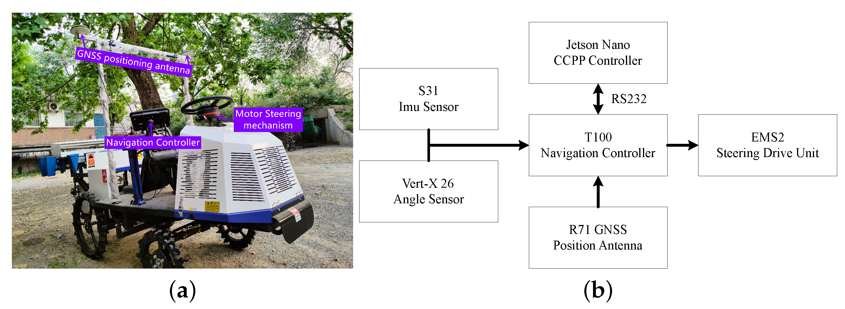
34], four fields with different shapes were used for evaluating the performance of the proposed improved-genetic-algorithm-based CCPP method, such as the algorithm convergence, the feasibility and optimality of the planned path. All the test experiments were performed on the transplanter (as shown in
Figure 12a, 2ZB-2B, DingDuo robot Co., Ltd., Baoji, China) with automatic navigation ability. The transplanter has the shape of 3050 × 2000 × 1750 (mm) (length × width × height). The automatic navigation system was the Beidou automatic navigation and driving system (AF301, Lianshi Navigation Technology Co., Ltd., Shanghai, China), which includes the double antenna satellite receiver (R71, Lianshi Navigation Technology Co., Ltd., Shanghai, China), the steering controller (EMS2, Lianshi Navigation Technology Co., Ltd., Shanghai, China), the angle sensor (Vert-X 26, Contelec AG, Bienne, Switzerland), the IMU (S31, Lianshi Navigation Technology Co., Ltd., Shanghai, China), and the vehicle-mounted information terminal (T100, Lianshi Navigation Technology Co., Ltd., Shanghai, China). The proposed CCPP method was deployed on the microprocessor (Jetson Nano, Nvidia Corp., Santa Clara), and the microprocessor connect with the vehicle-mounted information terminal through the RS232 interface. The connection between modules is shown in
Figure 12b.
3.1. Experiments Settings
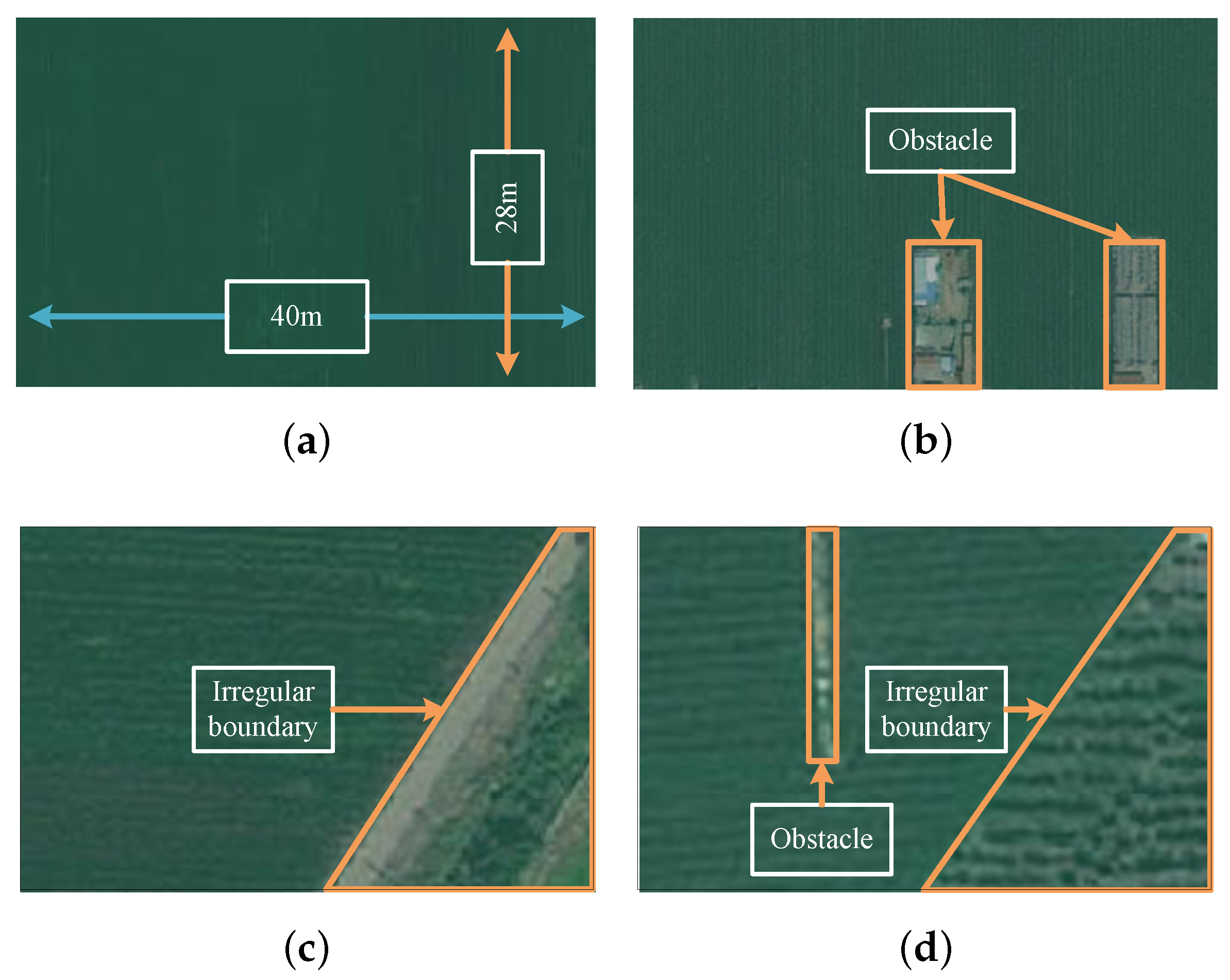
Environment map selection: One rectangular field A without obstacles (as shown in
Figure 13a, one rectangular field B with obstacles (as shown in
Figure 13b, one polygonal field C without obstacles (as shown in
Figure 13c, and one polygonal field D with obstacles (as shown in
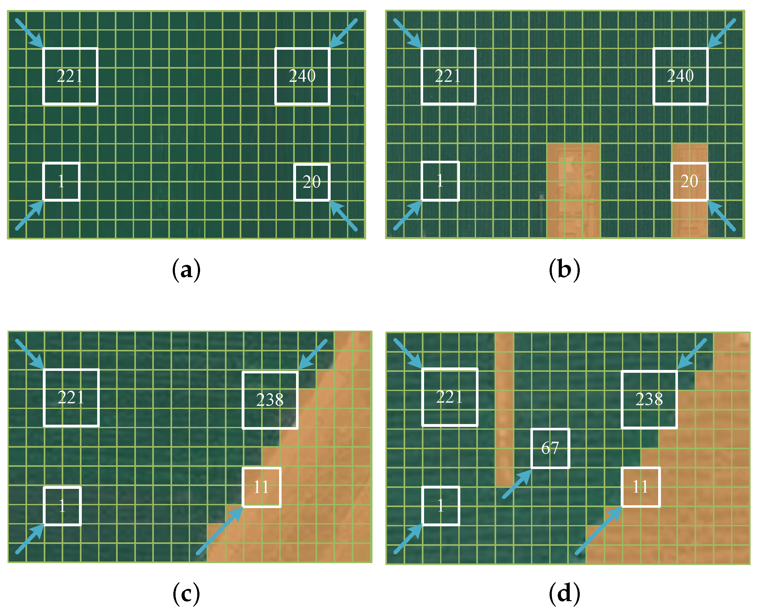
Figure 13d) were selected for testing the proposed CCPP method. The minimum bounding rectangles of the selected four fields have the same shape, i.e., 40 m long and 24 m wide. Then, the four fields were encoded as the grid maps (as shown in
Figure 14 using the method in
Section 2.1. The grid size was set to 2 m × 2 m according to the working width of the transplanter in
Figure 12.
In this paper, the selected four multi-topographic fields are processed through the environment map modeling based on the grid method, and the fields are rasterized according to the automatic driving agricultural robot with the work breadth of 2 m. Firstly, the fields are divided into grids with equal areas, with a grid area of
. Secondly, the boundary area and obstacle area are to be dilated into a regular-shaped map. Furthermore, finally, encoding the grid map to obtain four grid maps as shown in
Figure 14.
Parameters setting: The parameters of the proposed improved genetic algorithm were set to the same for all the selected testing fields. The number Q of the chromosome pairs in initial population was 200, the crossover probability of chromosomes was 0.5, the mutation probability of chromosomes was 0.01, and the number of iterations T was 5000. For the initial weights (i.e.,
,
and
) in (
1) of the repeated work area, the number of turns and the number of U-turns for fitness calculation were 0.3, 0.5, and 0.2, respectively. The elitist preservation strategy was adopted to ensure that the optimal chromosomes of each generation are inherited to the next generation, and the k in roulette selection was set to 1. The number of stable iterations M was set to 500; thus, when the fitness value was not changed for 500 consecutive times or the difference from the target value is less than 0.001, the algorithm will terminate in advance. The code of the algorithm proposed in this paper is written in C++ language, and run the program on a computer with Windows 11 operating system, Intel(R) Core(TM) i7-11800H processor, and 16GB memory. The average time of running 1000 iterations on a map with grid number 12 × 20 is 215 s. The running time will change with the number of grids and the number of iterations. When the number of grids and the number of iterations increase, the running time of the algorithm will increase accordingly.
3.2. Convergence Test of the Algorithm
To test the proposed multi-points mutation effect on the algorithm convergence and the global optimization-seeking ability, the single-point mutation was selected for comparison. The parameters for multi-points and single-point mutation were set to the same as in
Section 3.1, and the fitness values of the 1000 iterations were counted, as shown in
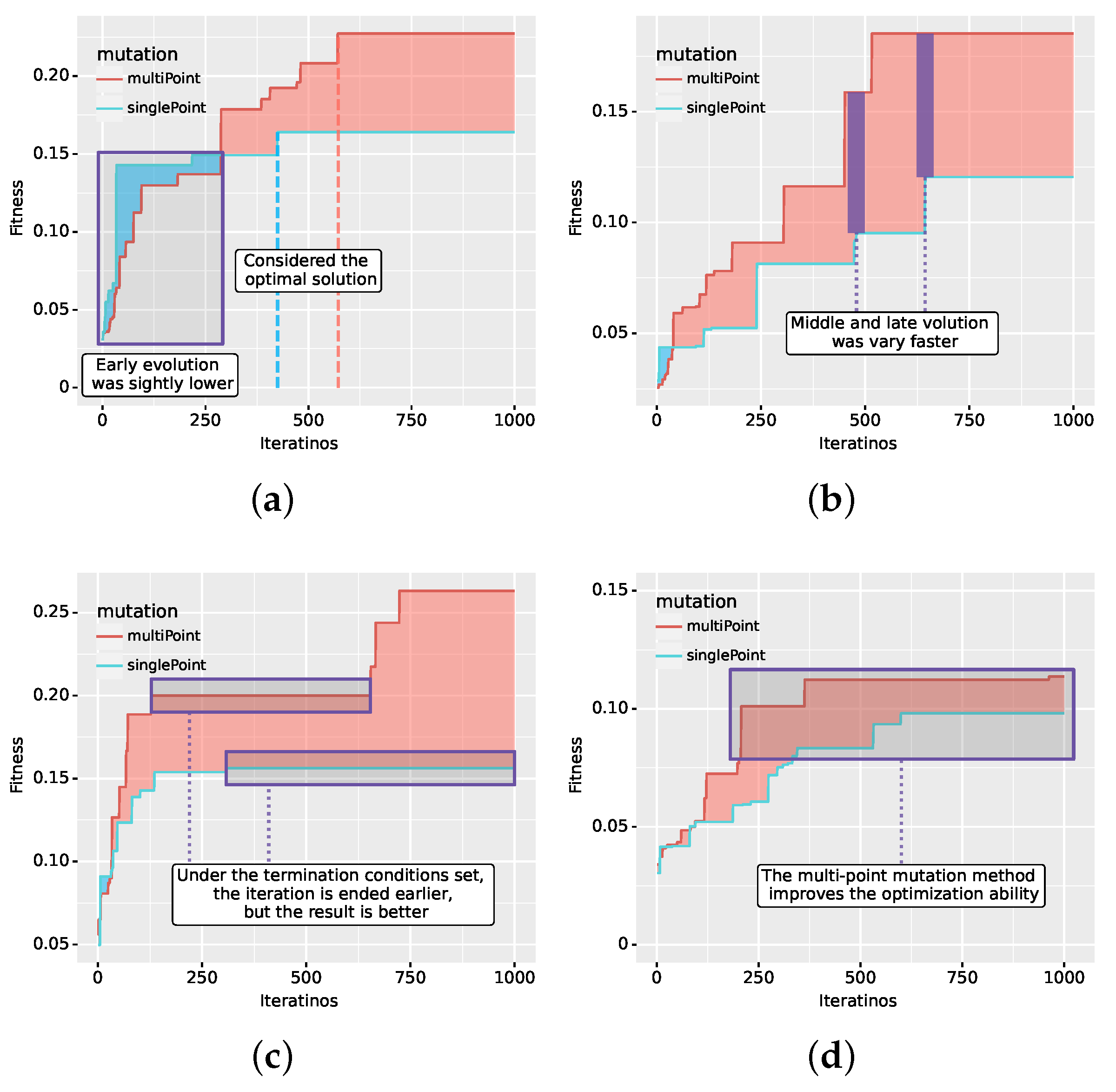
Figure 15. The results shown in
Figure 15 showed that the proposed multi-points mutation has a higher evolutionary efficiency than the single-point mutation. The fitness values of the 1000th iteration on the field A, B, C, and D calculated by the multi-points-mutation-based algorithm were 0.22727, 0.18519, 0.26316, and 0.11364, respectively, exceeding the fitness values calculated by the single-point-mutation-based algorithm, i.e., 0.16393, 0.12048, 0.15625, and 0.09804. This indicated that the global optimization-seeking ability of the multi-points mutation was increased comparing with the single-point mutation.
As shown in
Figure 15, the evolution speed of the improved genetic algorithm proposed in this paper was faster than that of the traditional genetic algorithm. This is because the order-preserving crossover method and multi-point mutation method can destroy the gene rank of the parent chromosome to the greatest extent, which can accelerate the algorithm to overstep the local extremum. As shown in
Figure 15a,b, in the regular-shaped field experiment, the multi-point mutation method has a stronger search ability than the single-point mutation method in both field A and B, especially in the field with obstacles (i.e., Field B). As shown in
Figure 15c, in the experiment of irregular-shaped field C, although the multi-point mutation method stopped earlier than the single-point mutation method, it has a higher fitness value. As shown in
Figure 15c,d, the multi-point mutation method improves the optimization ability of the algorithm at the later stage, and can find a better solution than the single point mutation. In addition, these are indicated that the algorithm has a strong adaptability in both regular-shaped and irregular-shaped fields.
3.3. Path Feasibility Test of the Algorithm
For testing the feasibility of the planned path, the traditional genetic algorithm with one chromosome-based CCPP method was used for comparison. The paths (as shown in
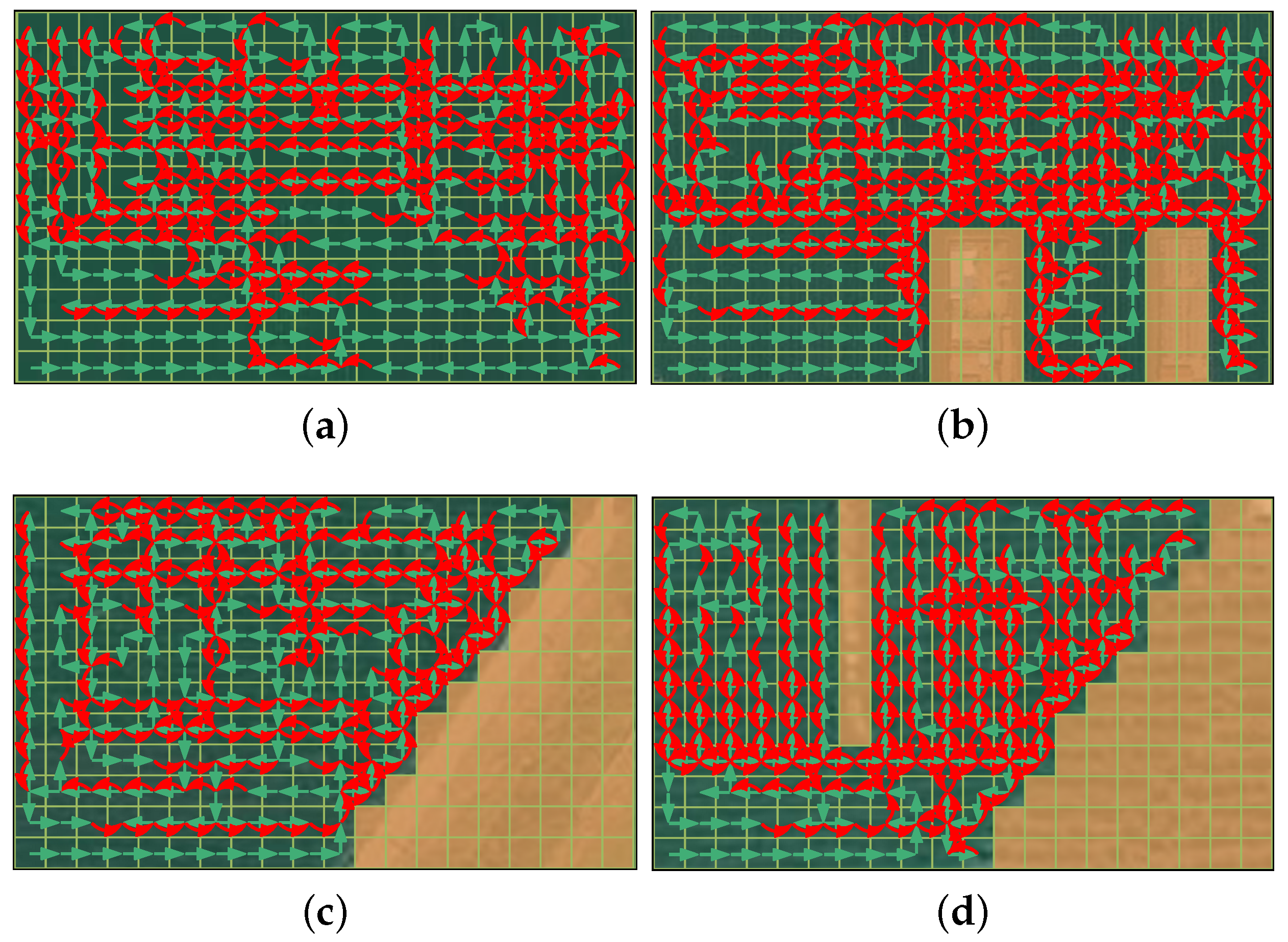
Figure 16) planned by the traditional genetic algorithm were disorganized for all testing fields. This is because the adjacent genes in the chromosome of the traditional genetic algorithm do not satisfy the 4-neighbor relationship, resulting in the excessive randomness of the planned path that the transplanting robot cannot follow. However, the proposed chromosome-pair-based genetic algorithm can plan the feasible path (as shown in
Figure 17, since all adjacent genes in chromosome
Y satisfy the 4-neighbor relationship with each other. The chromosome
Y represents a complete coverage path that the transplanting robot can follow.
3.4. Path Optimality Test of the Algorithm
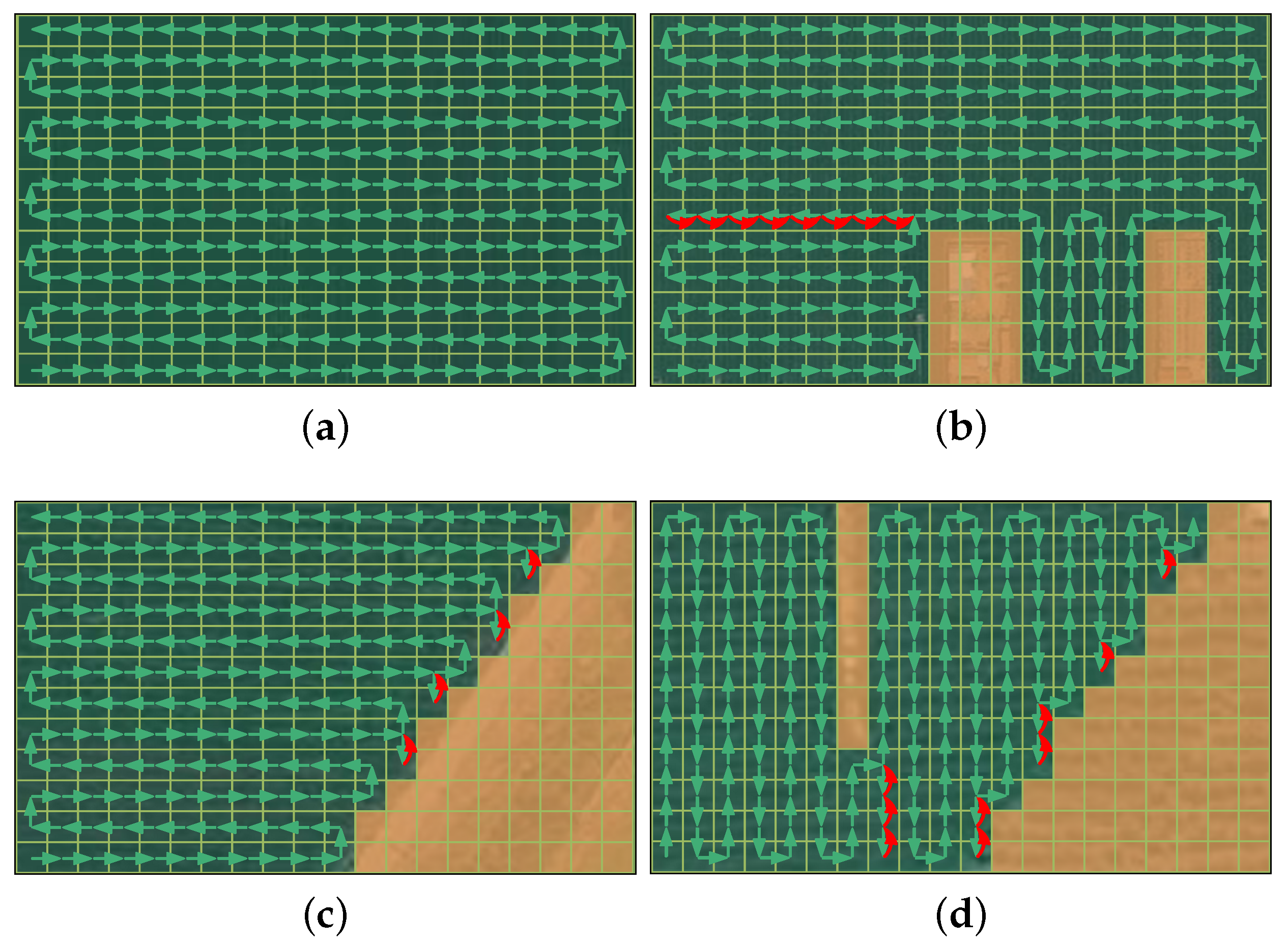
To test the optimality of the path planed by the proposed improved-genetic-algorithm-based CCPP method, the boustrophedon-based complete coverage method was used for comparison, and its planned path was shown in
Figure 18. Its basic idea was to use the “bow” type search method to cover the field, i.e., the transplanting robot works back and forth along the longest edge of the field. Furthermore, when encountering an obstacle, it moves a grid up to cross the obstacle, then returns to the previous working path. If the field boundary was reached, it moves back. The above steps were repeated until all the field were covered.
3.5. Experimental Results in Real Transplanting Robot
As shown in
Figure 18, it can be seen that the complete coverage path generated by the boustrophedon algorithm is more regular, showing a “bow” type operation pattern; however, there are more repetitive operation area and the number of U-turns. The complete coverage path generated by the proposed method (
Figure 17) has less repetitive operation area and number of U-turns. We use the transplanting robot shown in
Figure 12 to test the complete coverage operation in four multi-terrain fields using the boustrophedon method and the method in this paper, and the final energy consumption in the field is calculated by calculating the percentage drop of battery voltage. Field A is a barrier-free rectangular area, and the planning paths of boustrophedon method and this paper are the same, and there is no significant change in each index. Field D is an barrier irregular-shaped area, the area of repeated operation and the number of U-turns decreased significantly. In addition, as shown in
Table 2, the comprehensive energy consumptions of the boustrophedon method in four multi-topographic fields are 29%, 71%, 56%, and 85%, respectively. Furthermore, the comprehensive energy consumptions of the method in this paper are 29%, 66%, 51%, and 72%, respectively. This is because the method in this paper focuses on the complex farming environment, such as irregular-shaped boundary and obstacle in field, which is more suitable for field B, field C, and field D. Therefore, the CCPP method in this paper is more capable in complex fields.
Complete coverage path planning focuses on saving comprehensive energy consumption [
35], it can be seen from the comparison between the boustrophedon method and improved-genetic-algorithm-based method in
Table 3 and
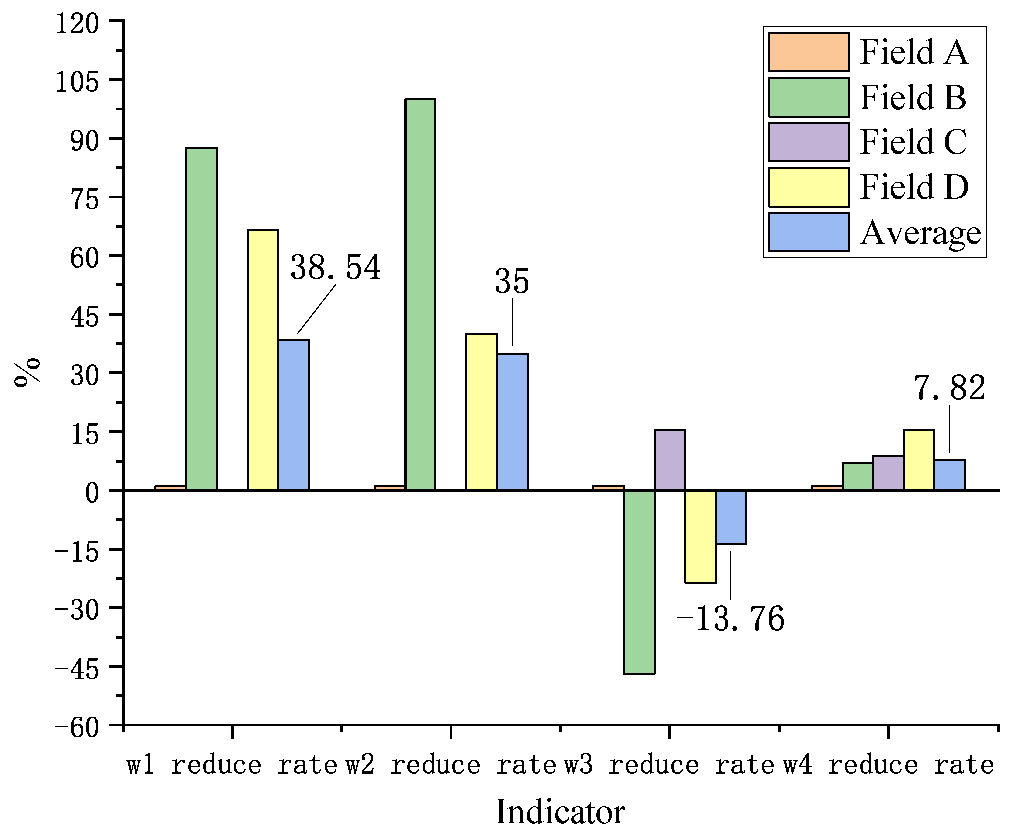
Figure 19. In four multi-topographic fields, all indicators are reduced except for a slight increase in the number of turns, which is due to the equilibrium adaptation fitness with multiple indicators. There will not be significant increases in the number of turns while reducing the area of repeated area and the number of U-turns. The advantage of the CCPP based on in this paper in field D is the most obvious, followed by field B and field C. In addition, with an average increase of 13.76% in the number of turns, the repetitive operation area, the number of turnarounds and the comprehensive energy consumption are reduced by 38.54%, 35.00%, and 7.82% on average. Although the CCPP method in this paper may increase the number of turns, the repeated operation area and the number of U-turns are decreased, and the comprehensive energy consumption is significantly reduced.
According to the above analysis, compared with the boustropredon method, the proposed method in this paper can minimize the repeated operation area and reduce the number of U-turns, which can help improve the operation efficiency of transplanting robot and reduce the operation energy consumption cost. It is more capable of planning a complete coverage path for the real operation of self-driving transplanting robots, which is more adaptable to the environment and has practical application value.
4. Conclusions
In this paper, the improved-genetic-algorithm is proposed to plan the complete coverage of the field of autonomous driving agricultural robot. Compared with the standard genetic algorithm, it has the following advantages. A chromosome adjustment method suitable for CCPP is designed to generate chromosome pairs, in which the number of chromosome genes before adjustment is the same, which is used for evolution operations, such as crossover and mutation. The number of adjusted chromosome genes is not necessarily the same, but each genes and their neighboring genes are consecutively adjacent in the grid-map, representing a feasible complete coverage path. Furthermore, we designed a multi-point mutation method, compared with single-point mutation, it can destroy the locus of the parent chromosome and has better global optimization ability. In order to verify the effectiveness of the algorithm proposed, the method in this paper and the boustrophedon method are used for CCPP for the four different types of actual fields. The complete coverage of the actual operation of agricultural robot reduces unnecessary mileage and improves operation efficiency. Next, this paper considers path planning for large-area fields to propose a new method that can handle large-scale grids. At the same time, the popular deep learning technology is used to improve the accuracy and efficiency of the algorithm, and multiple plots are studied to further improve the practicability of field path planning. The complete coverage path planning method based on grid method and improved genetic algorithm studied in this paper is mainly aimed at the field of self-driving agricultural robots. Of course, it can also be applied to broader scenarios, such as cleaning robots, demining robots, and plant protection drones and other fields.


