
Comparison of Modeling Methods for Off-Road Tires

1
Doctoral School of Mechanical Engineering, Hungarian University of Agriculture and Life Sciences, 2100 Gödöllő, Hungary
2
Department of Vehicle Technology, Hungarian University of Agriculture and Life Sciences, 2100 Gödöllő, Hungary
*
Author to whom correspondence should be addressed.
Machines 2023, 11(6), 658; https://doi.org/10.3390/machines11060658
Submission received: 30 April 2023
/
Revised: 11 June 2023
/
Accepted: 16 June 2023
/
Published: 19 June 2023
(This article belongs to the Section Vehicle Engineering)
Abstract
:Efficient navigation of off-road vehicles heavily relies on the ability to accurately model the interaction between the vehicle and the terrain. One of the most important parts of this interaction is the deformation of the terrain and the tire. Although high-precision methods like finite element method (FEM) simulation can be used for this purpose, they require significant computational power, which is impractical to install in a vehicle for real-time navigation purposes. Therefore, simplified and less-detailed models are essential for on-board installation in real-time applications. In this study, three two-dimensional static terrain–vehicle models are compared to a detailed FEM reference model, and the results are evaluated both from the perspective of accuracy and computational capacity requirements. The analysis sheds light on the effectiveness of each model in the real-time navigation of off-road vehicles.
1. Introduction
A fundamental part of navigation for vehicles in an off-road environment is to determine whether the vehicle is able to traverse a given part of the terrain. In the absence of a human driver, an autonomous vehicle has to evaluate the surrounding area, and plan the optimal route for the vehicle. When planning the optimal route, several factors can be taken into account (such as travel time and fuel consumption); however, considering the complexity of such navigation tasks, it is often deemed sufficient to find the shortest route along which the vehicle can move, while avoiding all non-traversable obstacles of the terrain [1,2]. These parts of the operational area are usually categorized as “go” or “no go”, referring to whether the vehicle can move through a given part of the area or not [3].
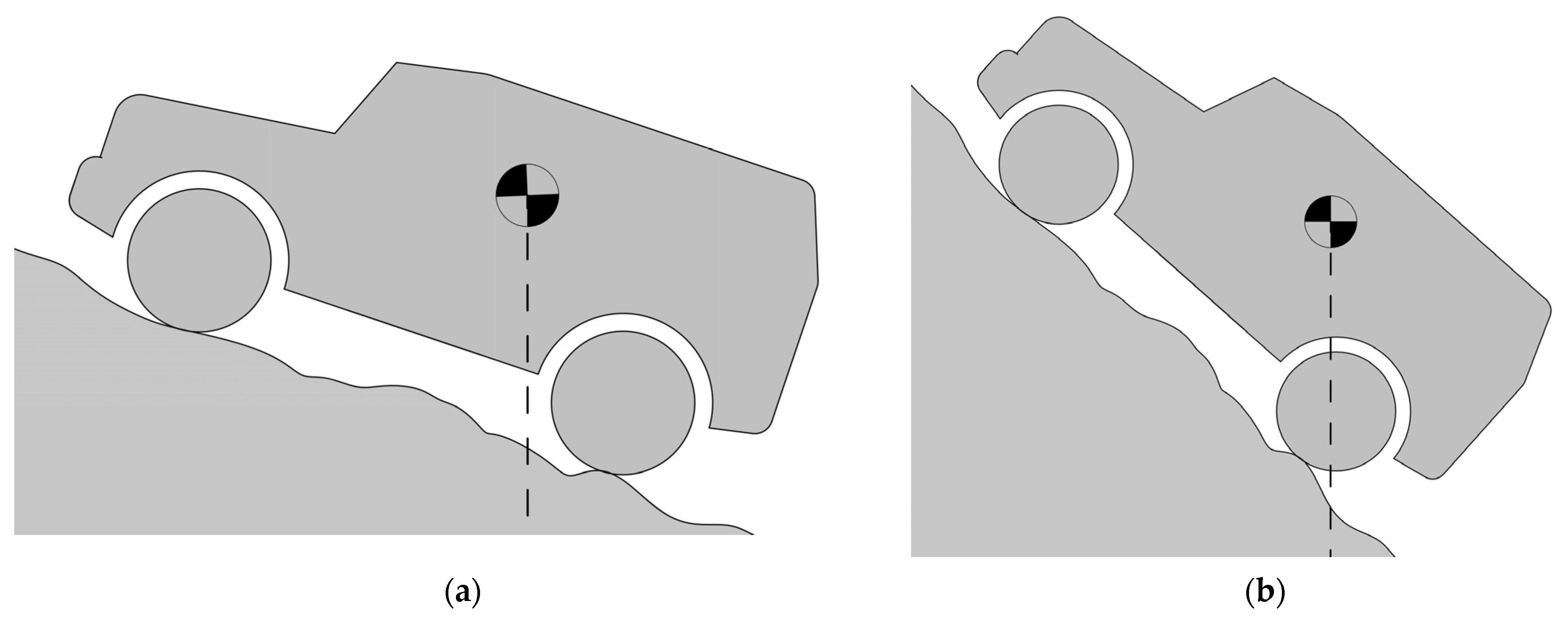
The terrain affects the dynamics of the vehicle in several ways. An obstacle can be non-traversable if the vehicle comes into contact with the obstacle through any part other than the wheels (namely, nose-in failure and hang up failure, see Figure 1) [4,5], or when the gravity acting on the center of mass falls outside the ground contact area (loss of stability, see Figure 2) [6]. Both of these factors depend on the geometrical position of the vehicle, which can be described using the coordinates of the wheel centers. For this reason, modeling the deformation of the tire and the terrain (soil) is very important. Apart from the stability and obstacle negotiation capability of the vehicle, the tire deformation affects the rolling resistance [7], and in agricultural applications, the pressure applied to the ground through the contacting area of the tire can also have an unfavorable effect on the soil from the perspective of seed growth [8].
Many already available and widely used methods are applicable to examining the interaction of the vehicle and the terrain, from the perspective of the tire–soil deformation. For example, there are several models used to characterize the deformation of the soil and the tire, and thus determine the total displacement as a function of the wheel or axle load. The most widely used models are the Bernstein model [9]:
the Saakyan model [10]:
and the Bekker model [11]:
where:
- —ground pressure [kPa];
- —sinkage [mm];
- —sinkage coefficient [-];
- —diameter of the contact area [mm];
- —the smaller characteristic dimension of the contact area [mm];
- —cohesion coefficient [-];
- —internal friction coefficient [-].
Most of these models are, at least partially, based on empirical data [12]. On the other hand, universal modeling methods such as finite element method (FEM) are also applicable for this purpose [13], or a combination of finite and discrete element method (DEM) can be used to model the characteristics of the rubber tire and the soil, respectively [14].
However, the applicability of these models is limited. The load–displacement equations are only applicable in the case of a flat undeformed ground surface, and not generally [15]. Considering that most of these models were created from an agricultural perspective, where the vehicles move on a surface with little to no macroscopic obstacles, general applicability was not an important aspect. Computer simulations, such as FEM and DEM, would be applicable for this purpose; however, they are highly limited by the available computational capacity. While this may not be an issue during scientific research, in real-time applications the available timeframe makes such simulation methods inapplicable, or at the very least, require a remarkably less detailed model. It also has to be taken into account that the available on-board hardware capacity—considering the operational conditions of an off-road vehicle, such as temperature and vibrations—is much less than that of a comparable desktop computer or server. Cloud-based remote computing theoretically could be a solution for this, but in many application fields, such as military or emergency services, the vehicle cannot rely on the availability of a high-speed network.
For these reasons, it is necessary to select an optimal modeling method (or create one, if none of the available models meets all criteria). An optimal model:
- is applicable in a general case;
- needs computational capacity that does not exceed the performance of readily available on-board hardware;
- is based only on theoretical methods and not empirical data, so as to be easily adapted for different conditions.
Determining the accuracy of a model is necessary when selecting the most suitable modeling method. With a known accuracy, the error can be easily compensated by applying a safety factor; thus, lower accuracy models can also be used reliably—even though the introduction of a safety factor partially reduces the number of theoretically traversable areas.
In this paper, three different modeling methods (including sub-types, seven models in total) are compared to an FEM reference model, and both the accuracy and the computational time of the models are compared.
2. Materials and Methods
2.1. Parameters of the Vehicle and Terrain
To compare the different models, a reference terrain profile was created. The terrain profile is based on a photogrammetric 3D scan of the agricultural test field at the Hungarian University of Agriculture and Life Sciences (Szent István Campus), modified to include a variety of different terrain features in a 20 m long section. The inclusion of a variety of terrain features in the reference profile ensures that the models are tested against a diverse range of obstacles, thereby providing a more accurate representation of real-world off-road conditions. The 3D mapping of the test terrain was carried out using a DJI Phantom 3 SE 4K quadrocopter. The point cloud, which is derived from the photogrammetric model, can be seen in Figure 3.
The point cloud model has a horizontal resolution of approximately 100 mm. For the modeling of the wheel–terrain interaction, the terrain profile was derived by extrapolating the discrete data points.
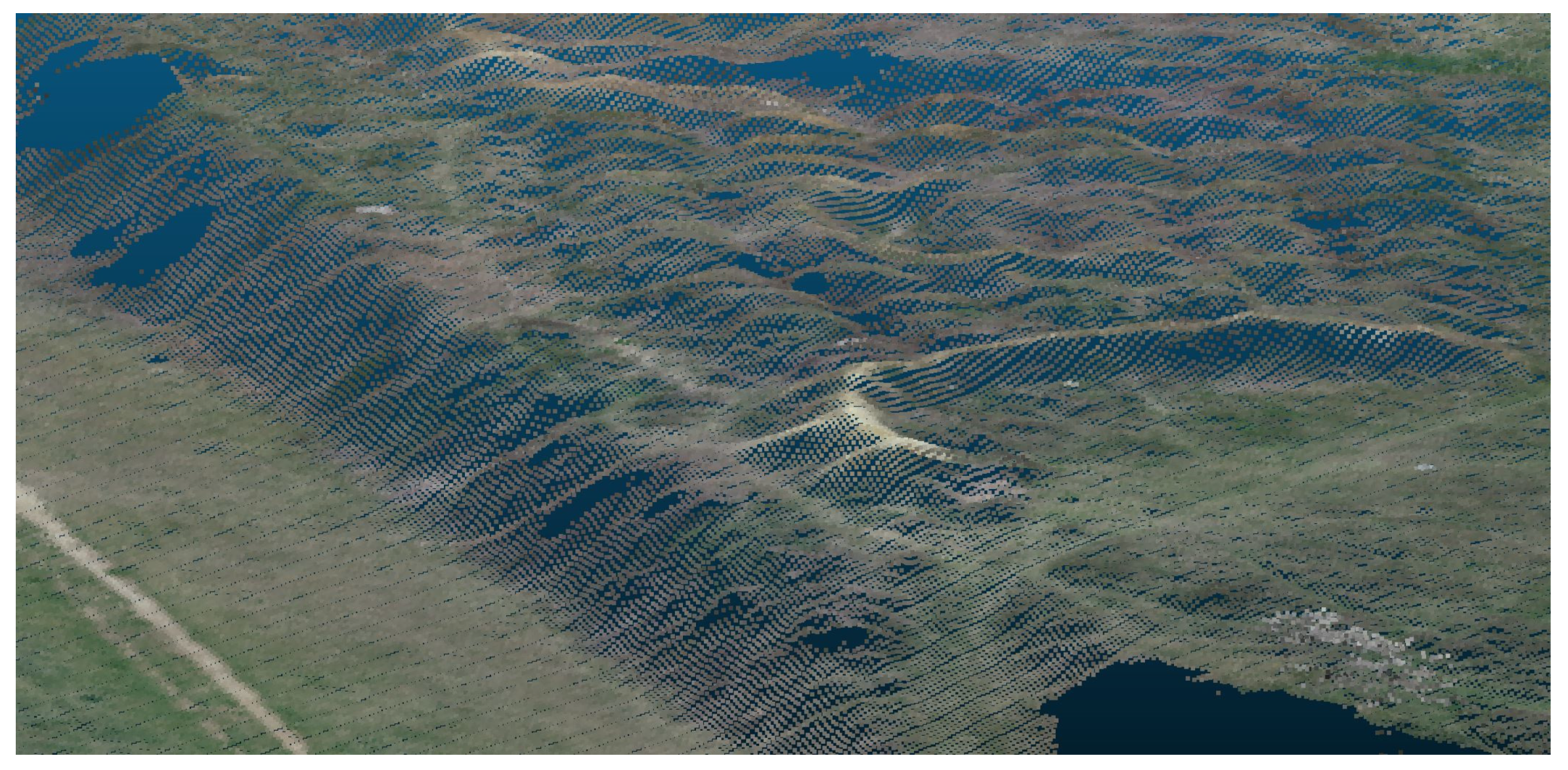
Considering that the longitudinal obstacle negotiation capabilities of off-road vehicles are far more important compared to the lateral ones, a two-dimensional terrain profile was used. For the three-dimensional FEM models, the same profile was used as a constant cross-section 3D solid. The position of the vehicle was determined at the same 50 points of the terrain by each of the following modeling methods. To describe the mechanical properties of the soil, the stress–strain characteristics shown in Figure 4 were used, comprising the typical values for a soft clay soil [16,17]. A soft soil was selected to examine the results at a relatively higher deformation, and thus a larger absolute error. The data shown in Figure 4 are a simplified characterization of the typical soil mechanical properties. Since the aim of the paper is not to model the wheel–terrain interaction in a specific case, but instead to compare the models in a general case, it was not important to obtain highly accurate values for the soil characteristics. Instead, approximate values were selected, while of course choosing the values from a realistic interval. The position (and thus the stability and obstacle negotiation capability) of the vehicle is dependent on the position of the four wheels (or two wheels, in the case of 2D modeling). The total displacement of each wheel depends on the wheel load, and the wheel load, in the case of a specific vehicle, depends on the pitch and roll of the vehicle, due to the change in weight distribution. This means that the geometrical position of the vehicle and the tire–soil deformation are mutually dependent variables. For this reason, an iterative process could be used for the calculations. However, considering that the expected deformation values are relatively small compared to the characteristic dimensions of the vehicle, this effect is deemed negligible and the weight distribution between the axles is considered to be approximately the same as it is in the non-deformed initial state.
Even without further examination of the effect of the elastic parameters on the model accuracy, it is trivial that a more rigid material pairing would mean smaller absolute error in the results. The hypothetical vehicle used in the simulations was a four wheeled vehicle with a 1.2 m wheelbase, and 600 mm × 200 mm × 250 mm (external diameter, width and rim diameter) solid rubber tires with a linear strain characteristic (with a Young’s modulus of 0.2 MP) [18], and a total mass of 500 kg, comparable to a typical small unmanned ground vehicle used in many fields. The tread pattern of the tire was neglected, as the research of Zeng et al. [19] has shown that the thread profile only causes a constant offset in the displacement. The effect of threads on other mechanical properties of solid rubber tires was also considered to be minor [20]. It has to be noted that, while these parameters are partially hypothetical, the aim of the research is not to model the interaction of a specific vehicle and terrain, but to compare modeling methods.
2.2. Reference Model
As a reference, a finite element model was used. The model takes into account the deformation of the terrain and the rubber tire; other parts of the vehicle were modeled as rigid bodies, as their only purpose in this model is to distribute the load to the tires. The model was created in Ansys Workbench R1 (2023). For better visualization, only a single wheel and rim is shown in Figure 5; a full model consists of a pair of these. The model created was a static model, meaning that the effect of rolling of the tire is not taken into account. Instead, the deformation of the tire and the terrain was modeled as a static state in each position, with only a vertical displacement of the wheel center allowed by the constraints. This is a necessary simplification, because, if a rolling tire model were used, the comparison to the other, simplified models (which do not take the effect of rolling into account) would not be possible. A dynamic modeling method would also be unrealistically complicated for this purpose. With static modeling, the conditions in each geometrical coordinate can be directly calculated; however, the introduction of dynamic modeling methods would mean that the speed of the vehicle and even the phase of vibration would have to be taken into account as independent variables. Aside from the fact that the introduction of two additional independent variables would make the results of this simulation much more complicated to compare, it must also be taken into account that the purpose of this research is to compare modeling methods for real-time purposes. In a navigation task of a vehicle under realistic conditions, these values (especially the phase angle of the vibration) cannot be calculated for a specific point or section further on the path of the vehicle when creating a mobility map. The phase angle of the vibration of the tire on off-road terrain can be influenced by various factors, including the earlier conditions encountered by the vehicle along its path. The effect of the speed and vibrations definitely influence the tire–soil interaction, but it must be considered that for off-road obstacles for which the obstacle negotiation capabilities of the vehicle are (nearly) exceeded—which is the main purpose of this research—the vehicle usually has a relatively small longitudinal speed. For these reasons, while a dynamic model would without doubt be more accurate, it was deemed to be much more complicated both from the perspective of the model itself and the comparison of the results. Therefore, it was decided that a static model would be more appropriate for this purpose.
For the modeling of tire–terrain interaction, a mathematical model also can be used. This would be expected to be less computationally intensive compared to a finite element model. However, such mathematical modeling methods cannot be created based on physical values alone; instead, results from either physical measurements or other simulations are required [21]. For this reason, while mathematical modeling can generally be useful, in this specific case, it is not an appropriate method for creating a reference model. Contrary to mathematical models, FEM simulation can be created based on the geometry and the mechanical properties of the included materials alone, which makes it the most suitable method for the purposes of this study.
In this research, the finite element model was used as a reference. The model can be considered theoretically perfectly accurate, as Deng has shown [22] that, based on actual measurements, finite element models of a non-pneumatic wheel have an error of approximately 5% from the perspective of wheel center displacement under operational loads, which is expected to be orders of magnitude smaller than the error of other methods compared in this research.
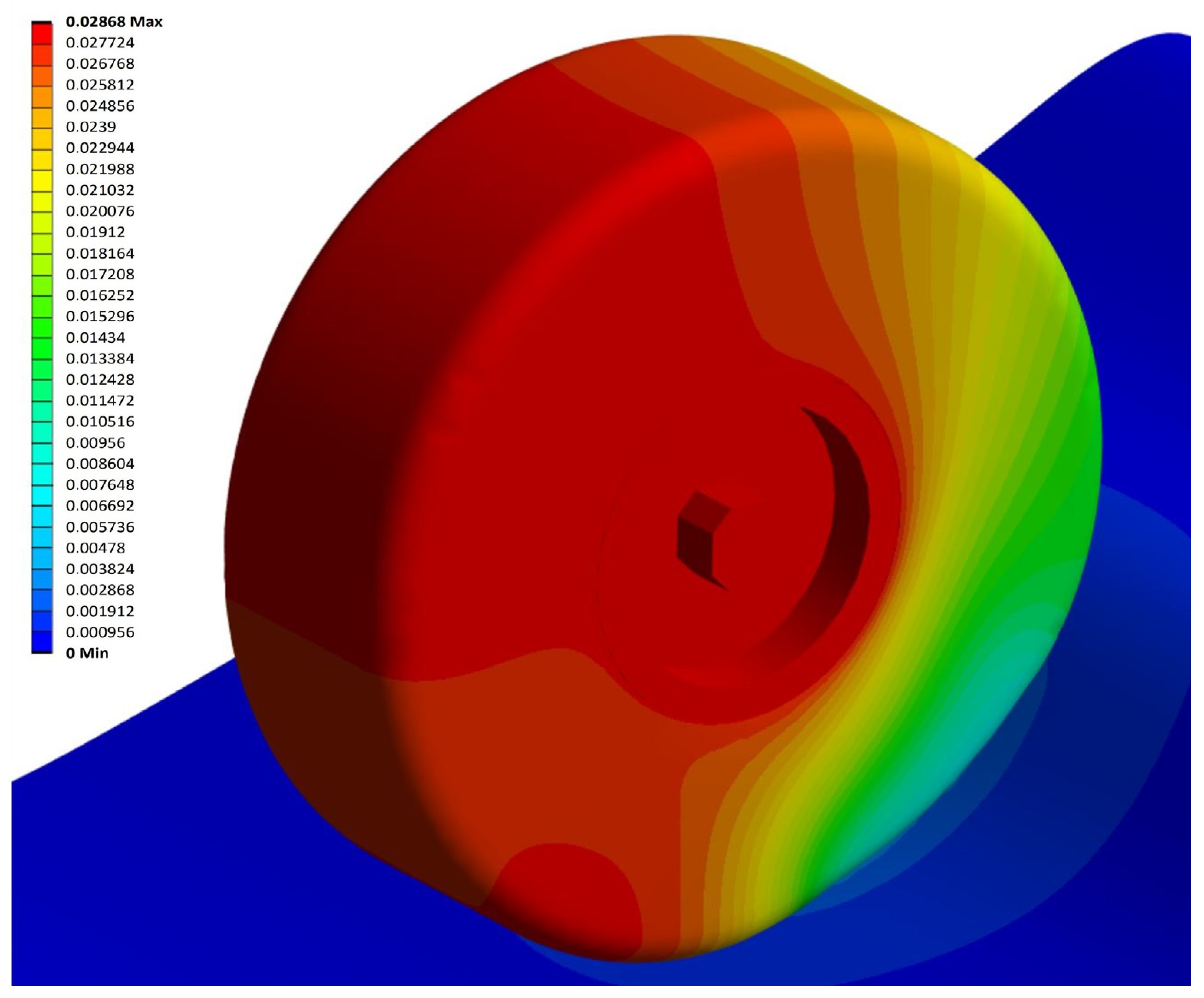
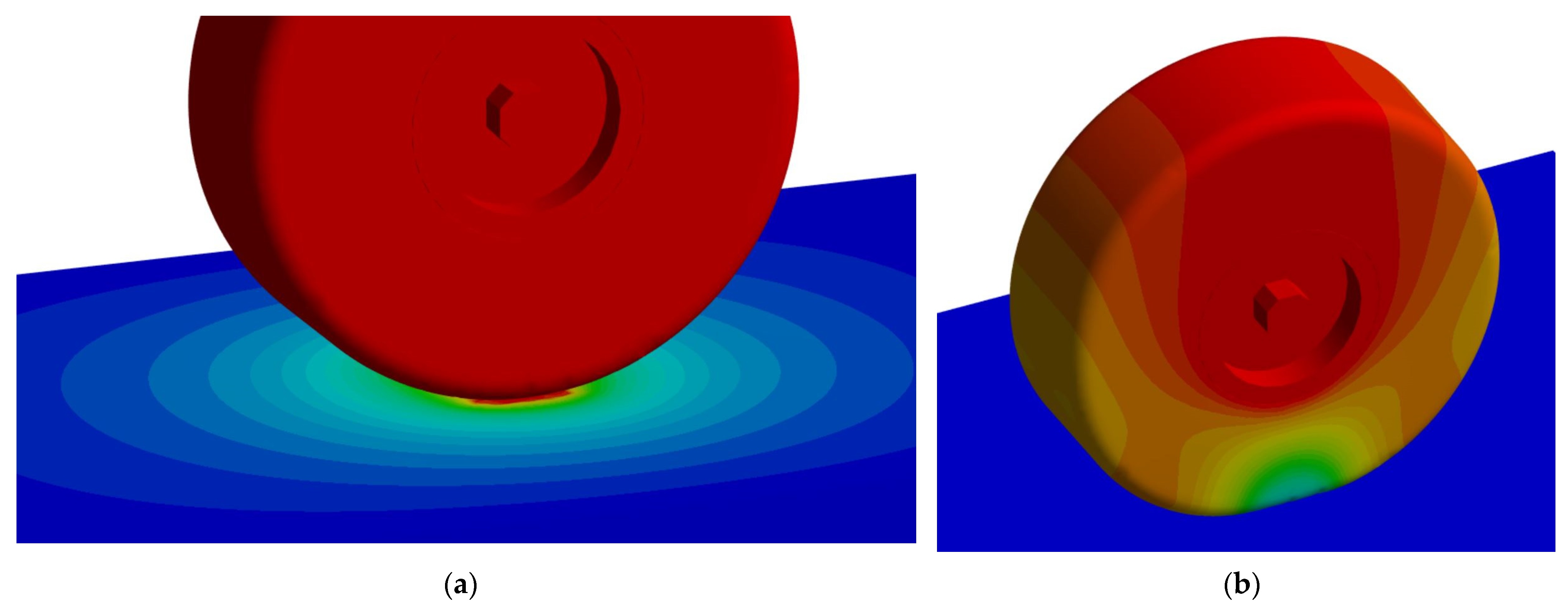
The reference model was created with a 20 mm meshing element size (triagonal) for the rubber tire, and an adaptive element-sized triagonal meshing for the terrain. The width and height of the modeled terrain section was chosen so that the effect of the load did not appear at the boundaries of the terrain section, and was thus equivalent to an infinite half space. The wheel load was determined and each point was based on the load shifting between the axles due to the pitch of the vehicle, with a 1250 N default load. The connection of the rigid rim and flexible tire was modeled as “Bonded”, the interaction of the tire and terrain as “No separation”. The solver method used for the reference simulation was “Conjugate gradient solver”, with a convergence tolerance of 10−8. The number of solver iterations was in the range of 100 to 150. The meshing of the FEM model and the results of a simulation can be seen in Figure 5b and Figure 6, respectively. The visualization of one of the reference simulations (Figure 6) shows the gradual displacement of both the wheel and the soil. As can be seen, the displacement of the rigid rim is constant at each point of the rim, and this displacement (which is the same as the axle displacement of the vehicle) is referred to as the wheel displacement in later parts of the study.
2.3. Finite Element Models
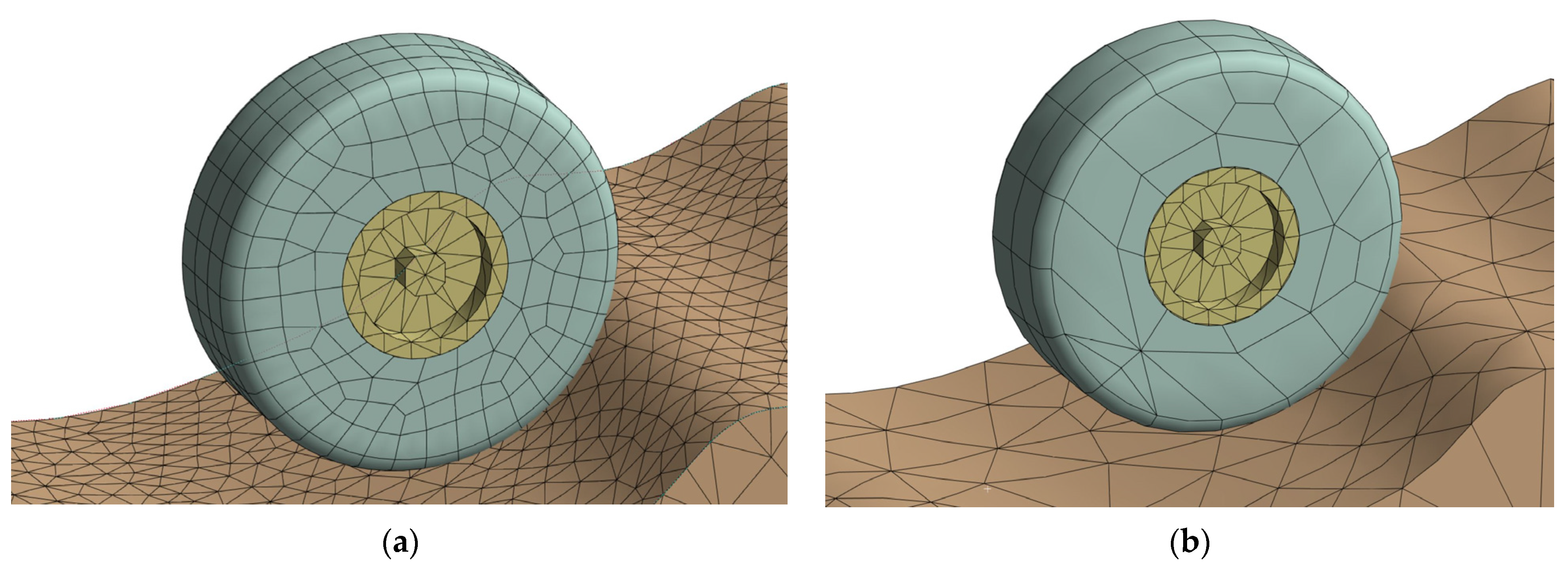
Apart from the one used as reference, two other, less detailed finite element models were examined and compared to the reference model. The FEM 1 and FEM 2 models had a decreased meshing resolution of 5 and 15 cm, respectively. As these models were identical to the reference model in every respect apart from the meshing resolution, including the mechanical material properties, the solver settings, and all other aspects of the FEM method, these models are not discussed in detail. The reduced resolutions of 5 and 15 cm changed the total node number from approximately 80,000 to 14,000 and 4000, respectively. The finite element models with a reduced meshing resolution can be seen in Figure 7a,b.
2.4. Linear Model
The simplest model which can be used assumes that the displacement of the axle is the same on any part of the terrain as it would be on a perfectly flat, horizontal terrain section, under the same load. This means that, compared to the position of the axle aster, the deformation can be derived from the theoretical non-deformed position and a load-dependent constant, which can be derived from a look-up table created by using the reference model. It was found that—within the load interval examined here—the axle displacement was linear to the vertical force, with a theoretical stiffness of 22.6 N/mm. The stiffness was acquired by gradually increasing the wheel load of the reference model up to 1250 N in 5 steps on a flat and horizontal terrain section, and a linear characteristic was fitted for these 5 force-displacement value pairs. In this method (which is more of an estimation method and not a simulation), the simplified characteristic is similar to a Hooke element, or a spring, in other words. It is important to note that this estimation method is expected to have a relatively high accuracy on flat terrains; however, on terrain sections with a more complex shape, the accuracy of the estimation is expected to be low. This effect of the terrain shape on the model accuracy is not examined in detail in this paper, but it could be a further research possibility.
2.5. Parallel Element Model
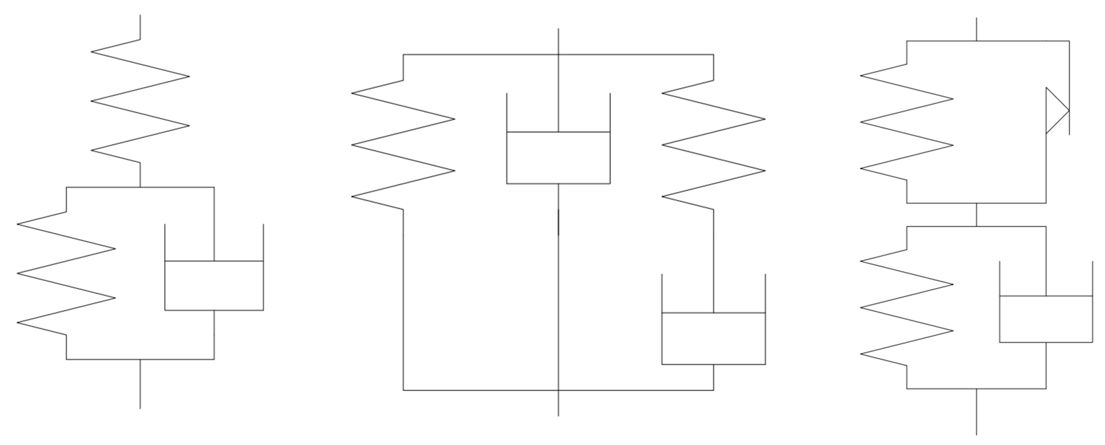
The rheological behavior of the soil and the rubber tire can be described by various models. The most commonly used soil rheological models are:
These models can be seen in Figure 8. The models are different in many ways, however, considering that only the static, steady state deformation is examined in this study, the velocity-dependent Newton elements of the models can be neglected. With this modification, all mentioned soil models could be simplified to a single linearly elastic Hooke element, or to a serially connected set of a Newton element and a Coulomb element. The latter will be used in this study to describe the behavior of the soil.
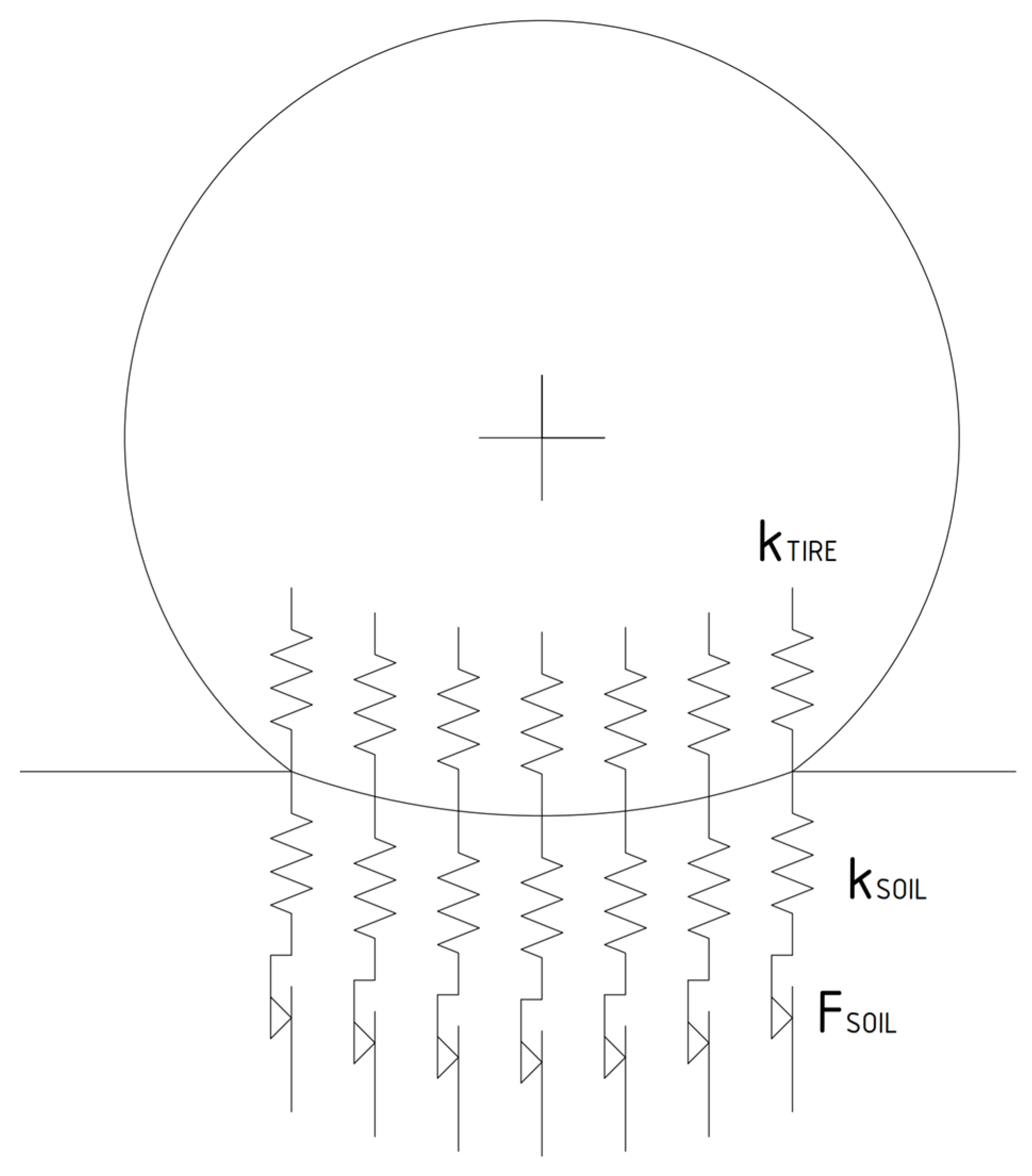
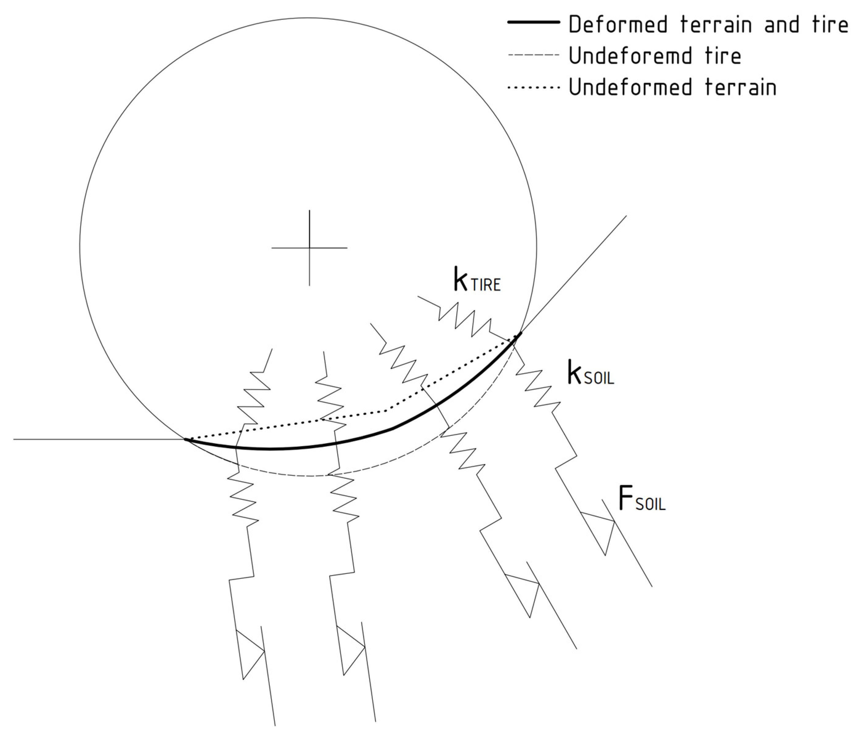
For similar reasons, the behavior of the rubber tire (which is usually characterized by the parallel connection of a linearly elastic Hooke element and a speed-dependent Newton element) was characterized using simple linearly elastic elements. The parallel element models combine the features of the finite element method and the conventional rheological models. Both flexible bodies are divided into a finite number of separate elements, however—contrary to finite element models—the elements of a body have no effect on each other. As Figure 9 shows, the model can be considered a set of parallel, vertical rheological elements with the same characteristics.
The rheological parameters of the tire and the soil elements were identified using the reference FEM model in two steps: by using a theoretically non-flexible tire to identify the soil parameters, and a non-flexible terrain to identify the tire parameters, as can be seen in Figure 10. In these two simulations, only the mechanical characteristics (of the rubber tire and the soil, respectively) were changed from flexible characteristics to rigid. With these changes, the simulation was carried out on a flat and horizontal terrain surface to identify the parameters for the parallel element model. After simulating the total displacement on the modified reference model, the parameters of the soil and tire elements were identified using the parallel element model with a reduced gradient method. It can be noted that, while the deformation under a given load obviously depends on the mechanical properties, the number of interacting soil–tire element pairs with a given wheel displacement do not, which makes the parameter identification simpler. When using a horizontal resolution of 1 cm, the following parameters were as follows: ktyre = 25.53 N/cm, ksoil = 168.9 N/mm, Fsoil = 92.3 N. It also has to be taken into account that the critical force of the soil models’ frictional part is only exceeded in a very small area of the terrain, which makes the parameter identification of the frictional elements critical force inaccurate; however, it also means that this parameter only has minor effects on the results.
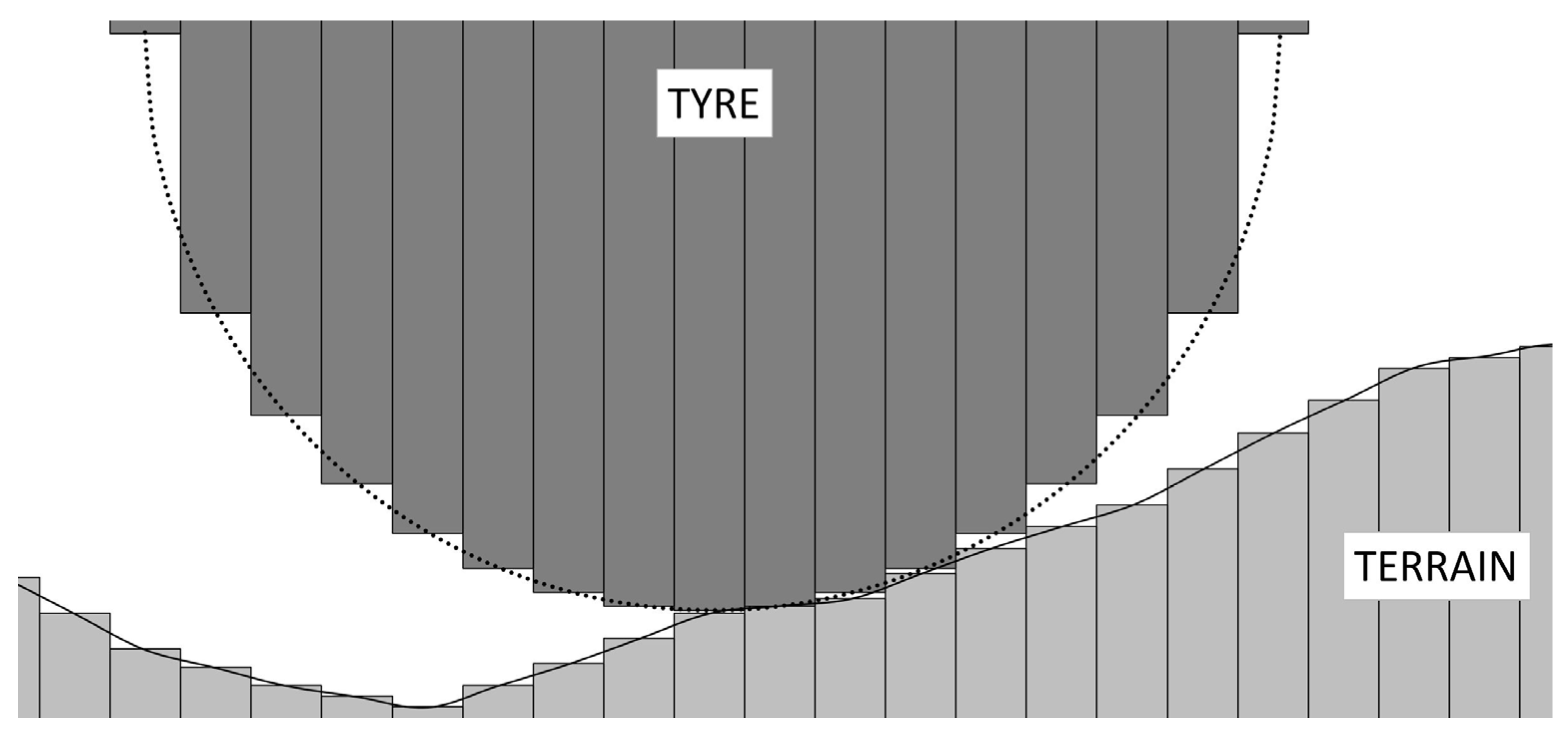
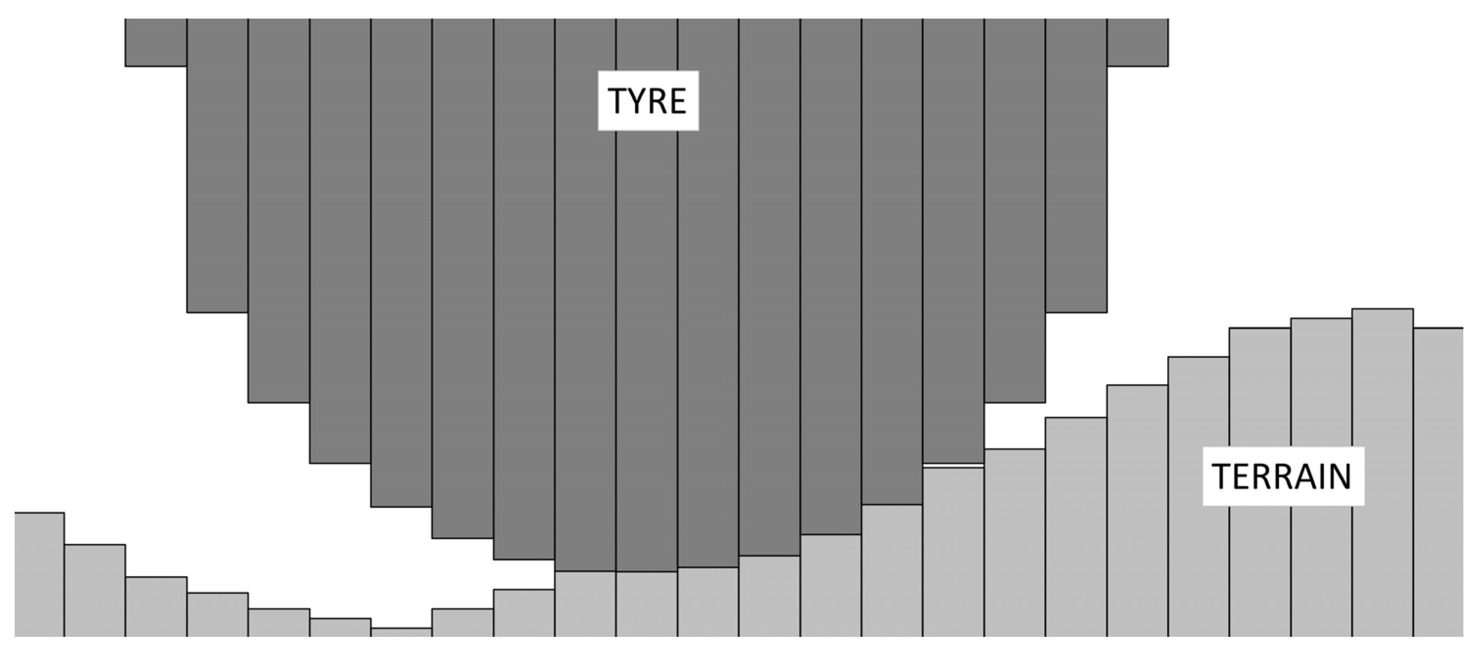
The model was applied using three different values of longitudinal element size: 10 mm, 25 mm, and 50 mm. These models are referred to as parallel element 1.1, 1.2, and 1.3, respectively. The visualization of the parallel element model in an actual terrain section can be seen in Figure 11 and Figure 12. The undeformed initial state (which can be seen in Figure 11) shows that the undeformed tire and terrain are connected only through a single rheological element. After applying the vertical load to the wheel, the connection surface increases (in this case to the width of seven elements), as can be seen in Figure 12. It can be noted that the contact area in the undeformed initial state is not a single element in every case, as it depends on the exact terrain profile. However, this does not affect the calculations. Due to the wheel load, the vertical coordinate of the wheel center (in a local, relative coordinate system) changed from 2.4768 m to 2.4509 m, which means a total wheel displacement of approximately 26 mm.
The software implementation of both parallel element models was carried out in Python 3. The rheological properties of the connecting tire–terrain element pairs were simplified to a parallel set of a Hooke and a Coulomb element. The resultant elastic coefficient can be calculated as
The resultant elastic coefficient of the parallel element model, in the case of a 10 mm element width, is kRES = 22.17 N/cm, with the frictional element of the soil keeping the original value of Fsoil = 92.3 N. Using this resultant rheological characteristic for the element pairs, the wheel displacement was calculated with an iterative process, since the number of the acting rheological element pairs depends on the displacement and so a simple algebraic equation could not be used. From the undeformed initial condition, the wheel displacement was increased in 1 mm increments, until the calculated total vertical force of the acting element pairs exceeded the nominal wheel load. The final wheel displacement value was calculated using linear interpolation between the two adjacent discrete displacement values.
2.6. Parallel Element Model 2
The second type of parallel element model used was similar to the first model in many ways. The main difference is that, in the second model, the rheological elements are not vertical, but perpendicular to the (undeformed) surface of the terrain and the tire, as can be seen in Figure 13.
In all other respects, the model is identical to the parallel element 1.1 model, and the same rheological parameters were used.
3. Results
All five of the previously discussed methods were used at the selected points of the terrain profile. It was assumed that the finite elements model used as a reference is perfectly accurate in the sense that, while the error of the model is not zero, it is negligible compared to the errors of other, less detailed models. Table 1 shows the results for the average accuracy of the models compared to the reference finite element model, and the required computational capacity. Apart from the reference finite element model, the table includes results for two additional FEM models (which only differ from the reference in their decreased resolution), the linear model, and four different parallel element models. Since the exact computational time required for each simulation method would be hard to interpret, a more meaningful value, the “Relative computational time”, was used. The relative computational time is a proportional value (compared to the least capacity-intensive linear model), where the linear model has a relative computational time of 1 (100%). This means that the computation of the “Parallel element 2”-type simulation is approximately 20 times longer compared to the linear model, regardless of the computer specifications. The introduction of the relative value is necessary to exclude the significant effect of hardware performance on the computational time. The usage of the relative value is based on the assumption that the ratio of computational times for different models would be the same, regardless of the exact hardware. The computing time only refers to the runtime of the simulation itself and does not include the importation of the initial data, identification of the model parameters, and the exportation and visualization of the results.
The results show that the less computational capacity a modeling method needs, the less accurate it is. It is important to note that this statement is not true in general, just for the models compared in this study. Modeling methods that require higher computational capacity yet are still less accurate can also exist.
By examining the results, it can be seen that there is no “best” modeling method, as the more accurate models require consistently more computational capacity. However, there are models that are inferior from the perspective of their cost–performance ratio. For example, it can be seen that, if a parallel element 1-type model is used, it is not necessary to use a higher resolution than 50 mm, as it would not significantly improve the accuracy. The results show that, apart from the FEM models, the parallel element 2 model has the highest accuracy, and the computational time of said model falls in the same magnitude as the simpler parallel element 1 models. However, the possible practical implementation of the models should also be considered. The linear and parallel element models were created in Python 3 for the purpose of this research, and the same method can easily be integrated into a larger project, for example, the creation of a mobility map. However, the FEM simulations require a separate software, and for these reasons the requirement for automatized modeling simulations can limit the applicable software solutions. Another aspect of optimal model selection (which could be a possibility for future research) is the comparison of the same models on a different point cloud. In this research, the 3D model of the test area was created by a fixed (10 cm) sampling resolution, and the terrain profile was extrapolated from these points. However, when using some 3D mapping methods (for example LIDAR), only an unstructured point cloud can be obtained. As mentioned earlier, the deformation of the tire and the soil affects the mobility and stability of the vehicle in many ways. The accuracy of the examined models can be interpreted differently, depending on the purpose of the modeling. The error of even the less accurate models is small compared to the external dimensions of the vehicle, and, for example, only has a minor effect on the change in the load distribution between the axles due to the pitch of the vehicle. However, from the perspective of the obstacle negotiation capabilities of the vehicle, even these inaccuracies are significant. Considering that a typical small UGV, comparable to the one used in the simulations, usually has a ground clearance of no more than around 150–250 mm, even a 20–30 mm safety clearance would have a significant effect on the obstacle negotiation capabilities. Based on the results of this study, it would be possible to select an optimal modeling method for a specific application, making a compromise between the accuracy and the computational capacity. Apart from selecting an optimal method, the results can be useful to determine what safety margins should be used for the mobility models. The safety margin should be large enough to compensate all of the possible inaccuracies of the mobility models, but also as small as possible so as not to reduce the theoretically traversable parts of the operational area more than what is absolutely necessary.
4. Discussion
In this study, eight different terrain–tire interaction models were compared, both from a perspective of accuracy and computational capacity. Based on the results, it can be said that all of the examined models may have a use in some circumstances. It is not possible to select a “perfect” model, as a compromise has to be made between the accuracy of the model and the available computational capacity. The results of this study can be used to select the optimal model for a specific application. Additionally, it is planned to continue the research and create an iterative method combining some of these models, adaptively using the more detailed (and thus, computational-capacity-intensive) models only for the critical parts of the terrain, while less detailed models can be used on the other parts. In this study, it was not thoroughly examined whether a mathematical connection between the accuracy of the models and the terrain profile can be found. However, it was found that the error of the models was larger at points where the terrain profile has a high microscopic roughness and/or has a high slope. Further research of this phenomena could provide important results, which could be essential to create the earlier-mentioned combined models, as it could provide a method to determine which models should be used at any given part of the terrain.
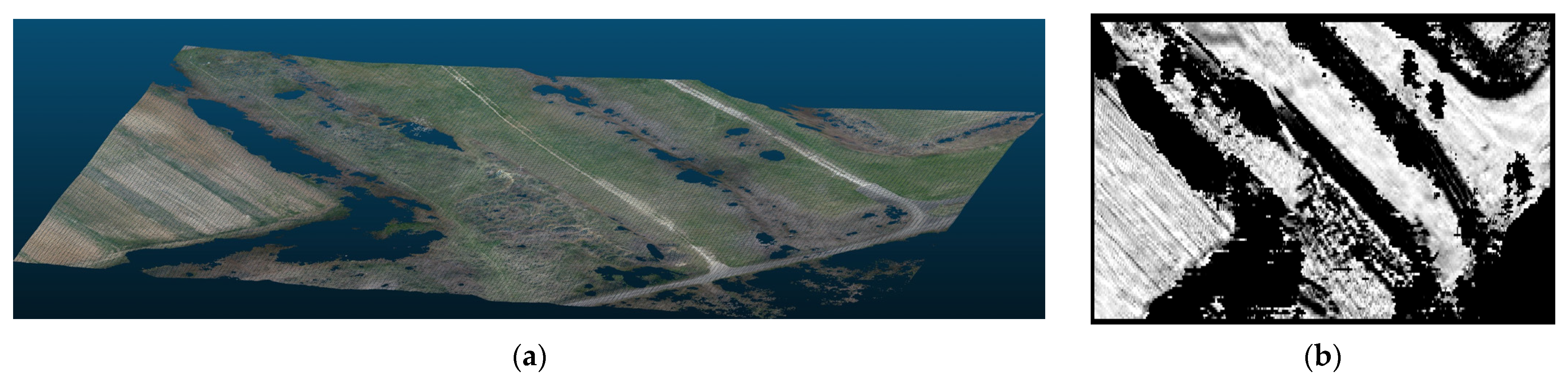
The wheel–terrain models compared in this study can be used to create a mobility map for off-road vehicle movement. An example of such a mobility map for the test field (Figure 14a) can be seen in Figure 14b. The mobility map shows the traversability of the terrain on grayscale, where non-traversable areas are marked in black and areas that are traversable without any obstacle in white. Based on such maps, an optimal route can be calculated with the appropriate mathematical minimum search algorithms.
Author Contributions
Conceptualization, D.K.; Methodology, D.K.; Software, D.K.; Writing—original draft, D.K.; Writing—review & editing, P.K.; Supervision, P.K.; Project administration, P.K. All authors have read and agreed to the published version of the manuscript.
Funding
Project no. 2022-2.1.1-NL-2022-00012 has been implemented with the support provided by the Ministry of Culture and Innovation of Hungary from the National Research, Development and Innovation Fund, financed under the 2022-2.1.1-NL funding scheme.
Data Availability Statement
The complete detailed datasets are generally not public due to the confidentiality requirements of the 2022-2.1.1-NL-2022-00012 research project. Soma data may be available upon request from the first author.
Acknowledgments
The drone-based 3D mapping of the test area was carried out with the contribution of the Department of Geodesy, Budapest University of Technology and Economics.
Conflicts of Interest
The authors declare no conflict of interest.
References
- Liu, Q.; Zhao, L.; Tan, Z.; Chen, W. Global path planning for autonomous vehicles in off-road environment via an A-star algorithm. Int. J. Veh. Auton. Syst. 2017, 13, 330–339. [Google Scholar] [CrossRef]
- Hong, Z.; Sun, P.; Tong, X.; Pan, H.; Zhou, R.; Zhang, Y.; Han, Y.; Wang, J.; Yang, S.; Xu, L. Improved a-star algorithm for long-distance off-road path planning using terrain data map. ISPRS Int. J. Geo-Inf. 2021, 10, 785. [Google Scholar] [CrossRef]
- Hua, C.; Niu, R.; Yu, B.; Zheng, X.; Bai, R.; Zhang, S. A Global Path Planning Method for Unmanned Ground Vehicles in Off-Road Environments Based on Mobility Prediction. Machines 2022, 10, 375. [Google Scholar] [CrossRef]
- Laib, L. Terepen Mozgó Járművek; Szaktudás Kiadó Ház: Budapest, Hungary, 2002. [Google Scholar]
- Lukács, T.J.; Vég, R.L. Az autonóm terepjáró eszközök. Műszaki Ktn. Közlöny 2022, 32, 107–116. [Google Scholar]
- Liu, J.; Ayers, P.D. Off-road vehicle rollover and field testing of stability index. J. Agric. Saf. Health 1999, 5, 59–72. [Google Scholar] [CrossRef]
- Karaftath, L.L. Rolling resistance of off-road vehicles. J. Constr. Eng. Manag. 1988, 114, 458–471. [Google Scholar] [CrossRef]
- Tardif-Paradis, C.; Simard, M.-J.; Leroux, G.D.; Panneton, B.; Nurse, R.E.; Vanasse, A. Effect of planter and tractor wheels on row and inter-row weed populations. Crop. Prot. 2015, 71, 66–71. [Google Scholar] [CrossRef]
- Bernstein, R. Probleme zur experimentellen Motorpflugmechanik. Der Mot. -Wagen 1913, 16, 199–206. [Google Scholar]
- Saakyan, S.S. Interaction of the Moving Wheel and Soil; Ministry of Agriculture of the Armenian SSR: Yerevan, Armenia, 1959. [Google Scholar]
- Bekker, M.G. Introduction to Terrain-Vehicle Systems. Part I: The Terrain. Part II: The Vehicle; University of Michigan: Ann Arbor, MI, USA, 1969. [Google Scholar]
- He, R.; Sandu, C.; Khan, A.K.; Guthrie, A.G.; Els, P.S.; Hamersma, H.A. Review of terramechanics models and their applicability to real-time applications. J. Terramechanics 2019, 81, 3–22. [Google Scholar] [CrossRef] [Green Version]
- Xia, K. Finite element modeling of tire/terrain interaction: Application to predicting soil compaction and tire mobility. J. Terramechanics 2011, 48, 113–123. [Google Scholar] [CrossRef]
- Kotrocz, K. Talaj Diszkrét Elemes Modellezése Talaj-Kerék Kölcsönhatásának Elemzéséhez. Ph.D. Thesis, Budapest University of Technology and Economics, Budapest, Hungary, 2019. [Google Scholar]
- Ding, L.; Gao, H.; Deng, Z.; Li, Y.; Liu, G. New perspective on characterizing pressure–sinkage relationship of terrains for estimating interaction mechanics. J. Terramechanics 2014, 52, 57–76. [Google Scholar] [CrossRef]
- López Bravo, E.; Herrera Suárez, M.; González Cueto, O.; Tijskens, E.; Ramon, H. Determinación de las Propiedades Mecánicas en un Suelo Arcilloso como Función de la Densidad y el Contenido de Humedad. Rev. Cienc. Técnicas Agropecu. 2012, 21, 5–11. [Google Scholar]
- Das, B.M. (Ed.) Geotechnical Engineering Handbook; J. Ross Publishing: Plantation, FL, USA, 2011. [Google Scholar]
- Schaefer, R.J. Mechanical properties of rubber. In Harris’ Shock and Vibration Handbook, 6th ed.; Piersol, A., Paez, T., Eds.; McGraw-Hill Companies Inc.: New York, NY, USA, 2010. [Google Scholar]
- Zeng, H.; Xu, W.; Zang, M. Experimental investigation of tire traction performance on granular terrain. J. Terramechanics 2022, 104, 49–58. [Google Scholar] [CrossRef]
- Jittham, P.; Sucharitpwatskul, S.; Siriruk, S.; Meesaringkarn, S. Finite Element Analysis of elastomer: Case study—Rolling resistances of pneumatic and solid tyres. IOP Conf. Ser. Mater. Sci. Eng. 2022, 1234, 012002. [Google Scholar] [CrossRef]
- Gorelov, V.; Komissarov, A. Mathematical model of the straight-line rolling tire—Rigid terrain irregularities interaction. Procedia Eng. 2016, 150, 1322–1328. [Google Scholar] [CrossRef] [Green Version]
- Deng, Y.; Zhao, Y.-Q.; Xu, H.; Zhu, M.-M.; Xiao, Z. Finite element modeling of interaction between non-pneumatic mechanical elastic wheel and soil. Proc. Inst. Mech. Eng. Part D J. Automob. Eng. 2019, 233, 3293–3304. [Google Scholar] [CrossRef]
- Gao, S.-W.; Wang, J.-H.; Zhou, X.-L. Solution of a rigid disk on saturated soil considering consolidation and rheology. J. Zhejiang Univ.-Sci. A 2005, 6, 222–228. [Google Scholar] [CrossRef]
- Józefiak, K.; Zbiciak, A. Secondary consolidation modelling by using rheological schemes. MATEC Web Conf. 2017, 117, 00069. [Google Scholar] [CrossRef] [Green Version]
- Komamura, F.; Huang, R.J. New rheological model for soil behavior. J. Geotech. Eng. Div. 1974, 100, 807–824. [Google Scholar] [CrossRef]
Figure 1.
Longitudinal stability of the vehicle: (a) stable position; (b) unstable position.

Figure 2.
Typical types of untraversable obstacles: (a) nose-in failure; (b) hang up failure.

Figure 3.
Point cloud geometrical map of the test field.

Figure 4.
Stress–strain characteristic of the simulated soil and tire.

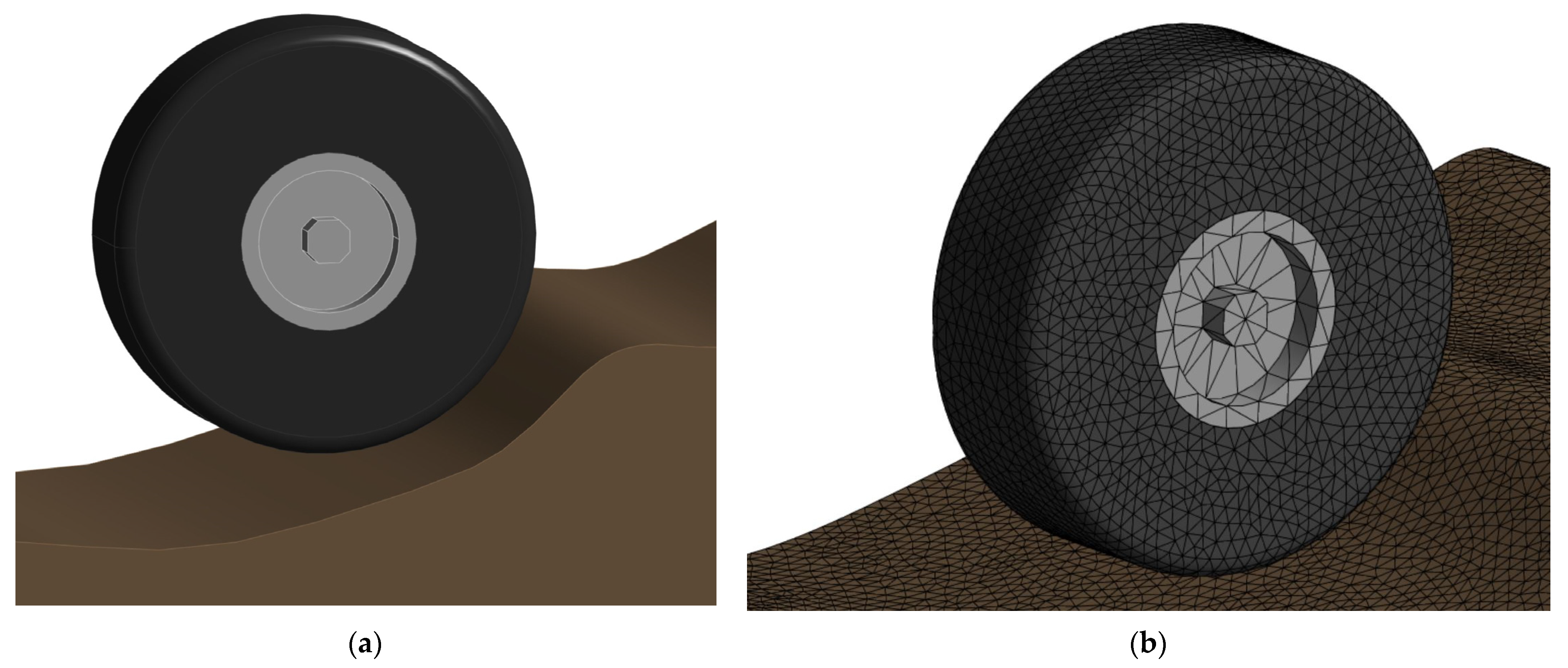
Figure 5.
Reference model: (a) geometrical model of the wheel on a 1000 mm wide terrain section; (b) tetrahedral meshing of the model.
Figure 5.
Reference model: (a) geometrical model of the wheel on a 1000 mm wide terrain section; (b) tetrahedral meshing of the model.

Figure 6.
Results of the reference finite element model, showing the displacement (m) under a 1250 N wheel load.
Figure 6.
Results of the reference finite element model, showing the displacement (m) under a 1250 N wheel load.

Figure 7.
FEM model with reduced 5 cm (a) and 15 cm (b) meshing resolution.

Figure 8.
Different rheological models of soil.

Figure 9.
Parallel element rheological model.

Figure 10.
Parameter identification using the reference model: (a) identification of the soil parameters using a rigid tire mode; (b) identification of the tire parameters on a rigid, perpendicular surface.
Figure 10.
Parameter identification using the reference model: (a) identification of the soil parameters using a rigid tire mode; (b) identification of the tire parameters on a rigid, perpendicular surface.

Figure 11.
Undeformed state of the parallel element rheological model.

Figure 12.
Deformed state of the parallel element model.

Figure 13.
Parallel element rheological model.

Figure 14.
An example for the practical applicability of the models: (a) 3D map of the test area (with the vegetation virtually removed); (b) greyscale mobility map of the area.
Figure 14.
An example for the practical applicability of the models: (a) 3D map of the test area (with the vegetation virtually removed); (b) greyscale mobility map of the area.


Table 1.
Results of the model comparison.
| Model | Avg. Accuracy (mm) | Rel. Computational Time (-) |
|---|---|---|
| Reference | - | 5199 |
| FEM 1 | 3.352 | 2172 |
| FEM 2 | 6.133 | 641 |
| Linear | 17.802 | 1 |
| Parallel element 1.1 | 10.764 | 12.38 |
| Parallel element 1.2 | 11.550 | 7.12 |
| Parallel element 1.3 | 11.684 | 4.23 |
| Parallel element 2 | 9.628 | 20.86 |
Disclaimer/Publisher’s Note: The statements, opinions and data contained in all publications are solely those of the individual author(s) and contributor(s) and not of MDPI and/or the editor(s). MDPI and/or the editor(s) disclaim responsibility for any injury to people or property resulting from any ideas, methods, instructions or products referred to in the content. |
© 2023 by the authors. Licensee MDPI, Basel, Switzerland. This article is an open access article distributed under the terms and conditions of the Creative Commons Attribution (CC BY) license (https://creativecommons.org/licenses/by/4.0/).
Share and Cite
MDPI and ACS Style
Körmöczi, D.; Kiss, P. Comparison of Modeling Methods for Off-Road Tires. Machines 2023, 11, 658. https://doi.org/10.3390/machines11060658
AMA Style
Körmöczi D, Kiss P. Comparison of Modeling Methods for Off-Road Tires. Machines. 2023; 11(6):658. https://doi.org/10.3390/machines11060658
Chicago/Turabian StyleKörmöczi, Dávid, and Péter Kiss. 2023. "Comparison of Modeling Methods for Off-Road Tires" Machines 11, no. 6: 658. https://doi.org/10.3390/machines11060658
Note that from the first issue of 2016, this journal uses article numbers instead of page numbers. See further details here.