
Reconfiguration Analysis and Characteristics of a Novel 8-Link Variable-DOF Planar Mechanism with Five Motion Modes


Abstract
:1. Introduction
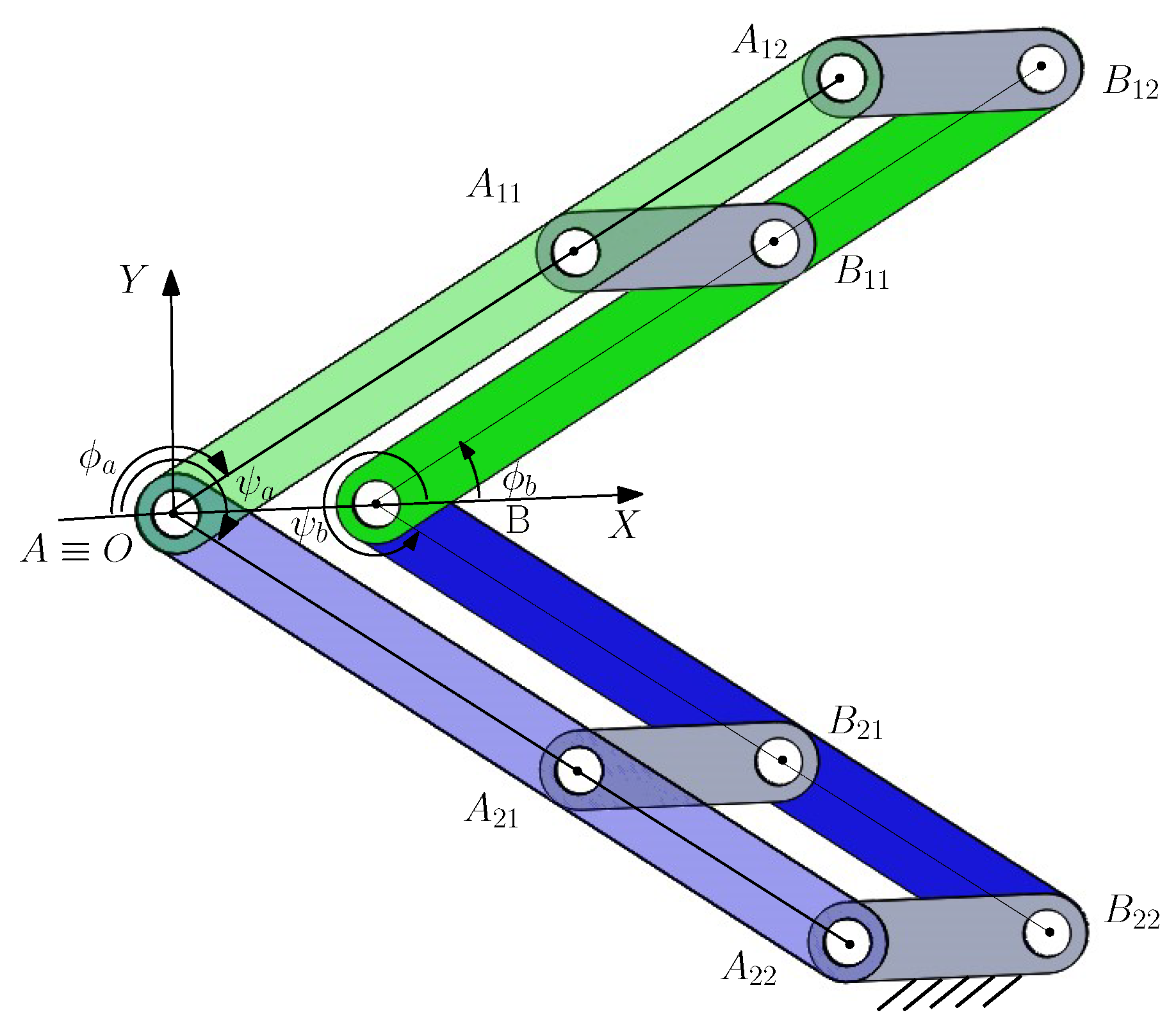
2. Geometric Description of a Novel 8-Link Variable-Dof Planar Mechanism
3. Kinematic Equations
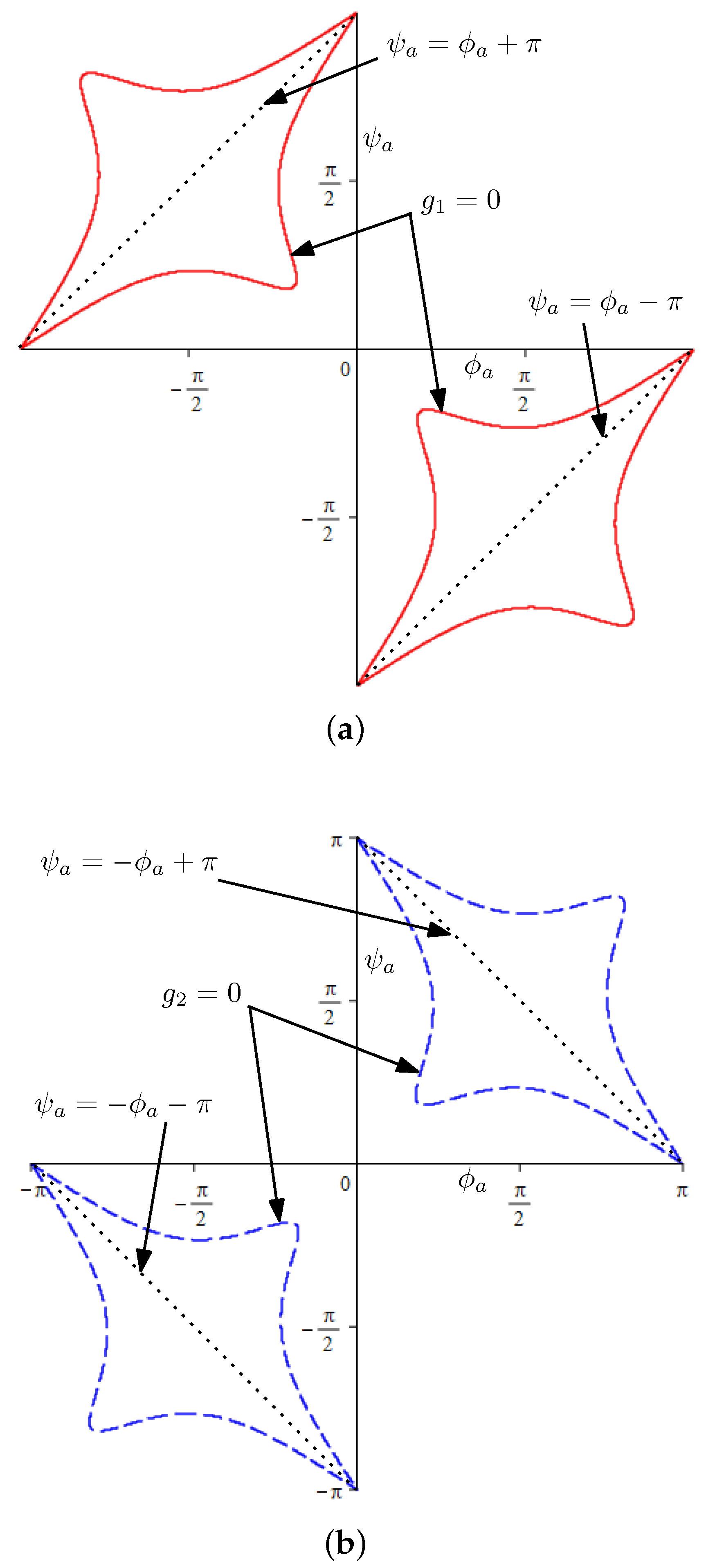
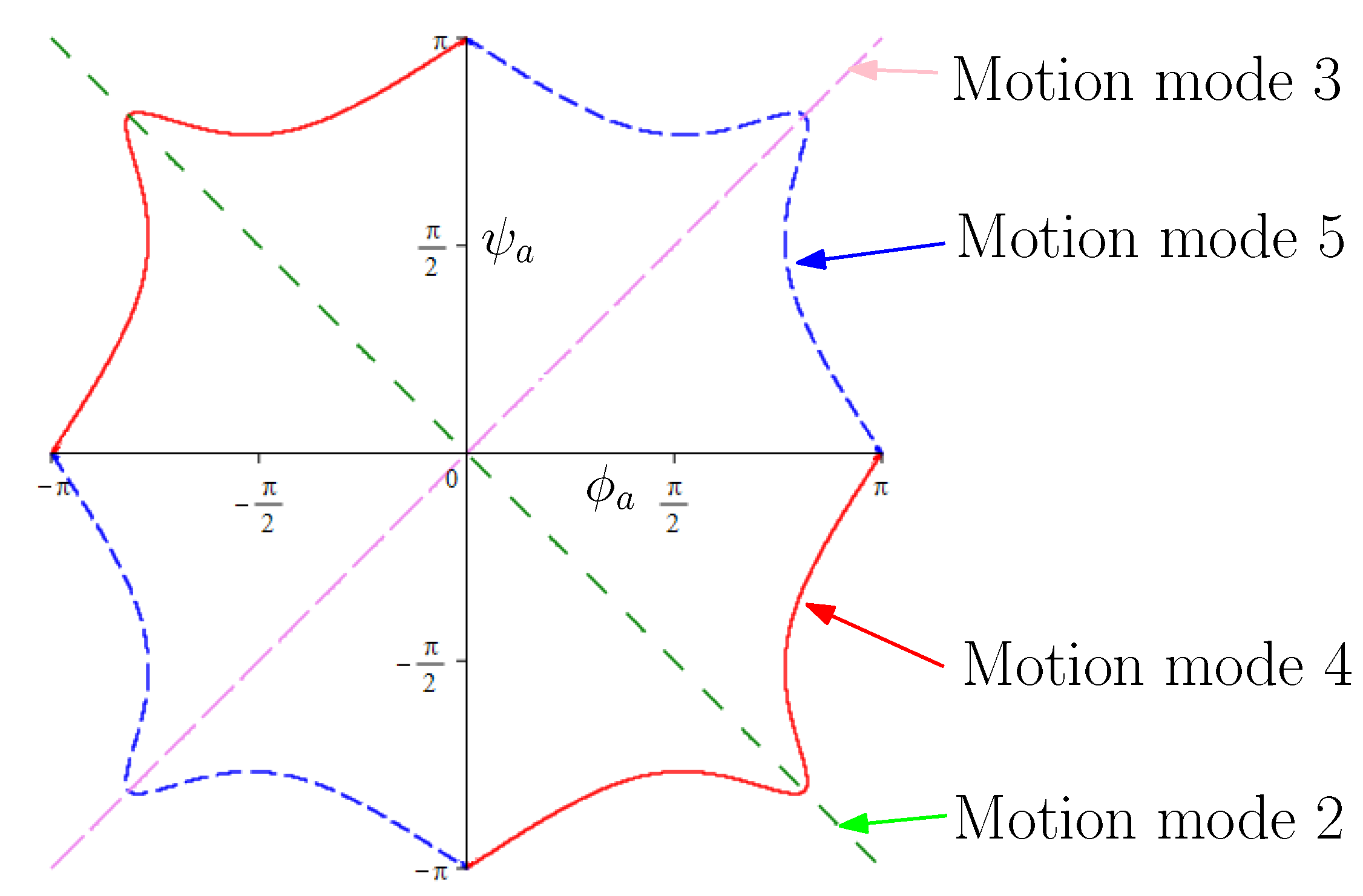
4. Motion Mode Analysis of an 8-Link Variable-Dof Planar Mechanism Using a Hybrid Approach
5. Transition Configuration Analysis of the 8-Link Variable-Dof Planar Mechanism
6. Reconfiguration of the Variable-Dof 8-Link Planar Mechanism
7. Conclusions
Supplementary Materials
Author Contributions
Funding
Data Availability Statement
Acknowledgments
Conflicts of Interest
Appendix A. Derivation of Equation (5)
Appendix B. Derivation of Equation (11)
- Step 1:
- Convert Equation (8) into a polynomial equation.Substituting and into Equation (8), we obtain a polynomial equation in and .where 72,900 215,280 72,900 63,661 12,122 63,661 57,600.
- Step 2:
- Calculate the primary decomposition of ideal , where and . The last two polynomials correspond to the trigonometric identities and .Calculating the primary decomposition of using computer algebra system software, such as MAPLE command PrimeDecomposition(J, ’removeredundant’), we havewhere the irreducible components, and , of are162,270288,30172,900168,881212,431 72,900 215,28072,90063,66112,12263,661576,00>, and 162,270 288,30172,900168,881212,43172,900 215,280 72,90063,66112,12263,661 57,600>.
- Step 3:
- Calculate the Gröbner basis for each irreducible component.Using the MAPLE command, Basis(J, tdeg(sa, ca, sb, cb)), we obtain the Gröbner basis of as.Similarly, the Gröbner basis of is.
- Step 4:
- Convert the polynomials in each of the irreducible components into trigonometrical functions.Substituting , , and into and simplifying the results, we obtain. i.e.,where .Similarly, we obtainwhere .
- Step 5:
- Divide the trigonometrical function in Equation (8) by the product of the trigonometrical functions obtained in Step 4.Divide g by , we can readily obtaini.e.
References
- Xi, F.; Dai, J.S.; Ding, X.; van der Wijk, V. Proceedings of the 5-th IEEE/IFToMM International Conference on Reconfigurable Mechanisms and Robots, Toronto, ON, Canada, 12–14 August 2021; Ryerson University: Toronto, ON, Canada, 2021. [Google Scholar]
- Herder, J.; van der Wijk, V. Proceedings of the 2018 International Conference on Reconfigurable Mechanisms and Robots (ReMAR 2018); IEEE: Piscataway, NJ, USA, 2018. [Google Scholar]
- Wohlhart, K. Kinematotropic linkages. In Recent Advances in Robot Kinematics; Lenarčič, J., Parenti-Castelli, V., Eds.; Kluwer Academic: Dordrecht, The Netherlands, 1996; pp. 359–368. [Google Scholar]
- Kovalev, M.D. Geometric theory of hinge devices. Russian Acad. Sci. Izv. Math. 1995, 44, 43–68. [Google Scholar]
- Galletti, C.; Fanghella, P. Single-loop kinematotropic mechanisms. Mech. Mach. Theory 2001, 36, 743–761. [Google Scholar] [CrossRef]
- Díez-Martínez, C.R. Mobility and Connectivity in Spatial Kinematic Chains. Master’s Thesis, Technological Institute of Celaya, Celaya, Mexico, 2005. (In Spanish). [Google Scholar]
- Kong, X.; Pfurner, M. Type synthesis and reconfiguration analysis of a class of variable-DOF single-loop mechanisms. Mech. Mach. Theory 2015, 85, 116–128. [Google Scholar] [CrossRef]
- López-Custodio, P.C.; Dai, J.S. Design of a variable-mobility linkage using the Bohemian dome. ASME J. Mech. Des. 2019, 141, 092303. [Google Scholar] [CrossRef]
- Feng, H.; Chen, Y.; Dai, J.S.; Gogu, G. Kinematic study of the general plane-symmetric Bricard linkage and its bifurcation variations. Mech. Mach. Theory 2017, 116, 89–104. [Google Scholar] [CrossRef]
- Lopez-Custodio, P.C.; Rico, J.M.; Cervantes-Sánchez, J.J.; Perez-Soto, G.I. Reconfigurable mechanisms from the intersection of surfaces. ASME J. Mech. Robot. 2016, 8, 021029. [Google Scholar] [CrossRef]
- Fanghella, P.; Galletti, C.; Giannotti, E. Parallel robots that change their group of motion. In Advances in Robot Kinematics; Lenarčič, J., Roth, B., Eds.; Springer: Dordrecht, The Netherlands, 2006; pp. 49–56. [Google Scholar]
- Liu, K.; Yu, J.; Kong, X. Structure synthesis and reconfiguration analysis of variable-degree-of-freedom single-loop mechanisms with prismatic joints using dual quaternions. ASME J. Mech. Robot. 2022, 14, 021009. [Google Scholar] [CrossRef]
- Kong, X. Type synthesis of variable degree-of-freedom parallel manipulators with both planar and 3T1R operation modes. In Proceedings of the ASME 2012 International Design Engineering Technical Conferences & Computers and Information in Engineering Conference, Chicago, IL, USA, 12–15 August 2012. DETC2012-70621. [Google Scholar]
- Coste, M.; Demdah, K.M. Extra modes of operation and self motions in manipulators designed for Schoenflies motion. ASME J. Mech. Robot. 2015, 7, 041020. [Google Scholar] [CrossRef]
- Zeng, Q.; Ehmann, K.F.; Cao, J. Design of general kinematotropic mechanisms. Robot. Comput. Integr. Manuf. 2016, 38, 67–81. [Google Scholar] [CrossRef]
- Zhang, K.; Dai, J.S. Screw-system-variation enabled reconfiguration of the Bennett plano-spherical hybrid linkage and its evolved parallel mechanism. ASME J. Mech. Des. 2015, 137, 062303. [Google Scholar] [CrossRef]
- Nurahmi, L.; Caro, S.; Wenger, P.; Schadlbauer, J.; Husty, M. Reconfiguration analysis of a 4-RUU parallel manipulator. Mech. Mach. Theory 2016, 96, 269–289. [Google Scholar] [CrossRef]
- Nurahmi, L.; Putrayudanto, P.; Wei, G.; Agrawal, S.K. Geometric constraint-based reconfiguration and self-motions of a four-CRU parallel mechanism. ASME J. Mech. Robot. 2021, 13, 433748391. [Google Scholar] [CrossRef]
- Kong, X. Classification of a 3-RER parallel manipulator based on the type and number of operation modes. ASME J. Mech. Robot. 2021, 13, 021013. [Google Scholar] [CrossRef]
- López-Custodio, P.C.; Müller, A.; Dai, J.S. A kinematotropic parallel mechanism reconfiguring between three motion branches of different mobility. In Advances in Mechanism and Machine Science. IFToMM WC 2019; Uhl, T., Ed.; Springer: Cham, Switzerland, 2019; pp. 2611–2620. [Google Scholar]
- Liu, Y.; Li, Y.; Yao, Y.-A.; Kong, X. Type synthesis of multi-mode mobile parallel mechanisms based on refined virtual chain approach. Mech. Mach. Theory 2020, 152, 103908. [Google Scholar] [CrossRef]
- Qin, Y.; Dai, J.S.; Gogu, G. Multi-furcation in a derivative queer-square mechanism. Mech. Mach. Theory 2014, 81, 36–53. [Google Scholar] [CrossRef]
- Kong, X. Variable degree-of-freedom spatial mechanisms composed of four circular translation joints. ASME J. Mech. Robot. 2021, 13, 031007. [Google Scholar] [CrossRef]
- Arponen, T.; Piipponen, S.; Tuomela, J. Kinematical analysis of Wunderlich mechanism. Mech. Mach. Theory 2013, 70, 16–31. [Google Scholar] [CrossRef]
- Wang, J.; Kong, X. A novel method for constructing multimode deployable polyhedron mechanisms using symmetric spatial compositional units. ASME J. Mech. Robot. 2019, 11, 020907. [Google Scholar] [CrossRef]
- Tian, C.; Zhang, D.; Tang, H.; Wu, C. Structure synthesis of reconfigurable generalized parallel mechanisms with configurable platforms. Mech. Mach. Theory 2021, 160, 104281. [Google Scholar] [CrossRef]
- Liu, R.; Li, R.; Yao, Y.-A.; Ding, X. A reconfigurable deployable spatial 8R-like mechanism consisting of four angulated elements connected by R joints. Mech. Mach. Theory 2023, 179, 105103. [Google Scholar] [CrossRef]
- Laliberté, T.; Gosselin, C. Construction, mobility analysis and synthesis of polyhedra with articulated faces. ASME J. Mech. Robot. 2014, 6, 011007. [Google Scholar] [CrossRef]
- Overvelde, J.; Weaver, J.; Hoberman, C.; Bertoldi, K. Rational design of reconfigurable prismatic architected materials. Nature 2017, 54, 347–352. [Google Scholar] [CrossRef] [PubMed]
- Yan, H.; Kuo, C. Topological representations and characteristics of variable kinematic joints. ASME J. Mech. Des. 2006, 128, 384–391. [Google Scholar] [CrossRef]
- Gan, D.; Dai, J.S.; Caldwell, D.G. Constraint-Based Limb Synthesis and Mobility-Change-Aimed Mechanism Construction. ASME J. Mech. Des. 2011, 133, 051001. [Google Scholar] [CrossRef]
- Jia, P.; Li, D.; Zhang, Y.; Yang, C. A novel reconfigurable parallel mechanism constructed with spatial metamorphic four-link mechanism. Proc. Inst. Mech. Eng. Part C 2022, 236, 4120–4132. [Google Scholar] [CrossRef]
- Li, Z.; Scharler, D.F.; Schröcker, H.-P. Factorization results for left polynomials in some associative real algebras: State of the art, applications, and open questions. J. Comput. Appl. Math. 2019, 349, 508–522. [Google Scholar] [CrossRef]
- Montes, A.; Wibmer, M. Software for discussing parametric polynomial systems: The Gröbner Cover. In Mathematical Software—ICMS 2014; Hong, H., Yap, C., Eds.; Springer: Berlin, Germany, 2014; pp. 406–413. [Google Scholar]
- Cox, D.A.; Little, J.B.; O’Shea, D. Ideals, Varieties, and Algorithms; Springer: New York, NY, USA, 2007. [Google Scholar]
- Husty, M.L.; Schröcker, H.-P. Kinematics and Algebraic Geometry. In 21st Century Kinematics; McCarthy, J.M., Ed.; Springer: London, UK, 2013; pp. 85–123. [Google Scholar]
- Wampler, C.; Sommese, A. Numerical algebraic geometry and algebraic kinematics. Acta Numer. 2011, 20, 469–567. [Google Scholar] [CrossRef]
- Shabani, A.; Porta, J.M.; Thomas, F. A branch-and-prune method to solve closure equations in dual quaternions. Mech. Mach. Theory 2021, 164, 104424. [Google Scholar] [CrossRef]
- Pellegrino, S. Structural computations with the singular value decomposition of the equilibrium matrix. Int. J. Solids Struct. 1993, 30, 3025–3035. [Google Scholar] [CrossRef]
- Song, C.Y.; Chen, Y.; Chen, I.-M. A 6R linkage reconfigurable between the line-symmetric Bricard linkage and the Bennett linkage. Mech. Mach. Theory 2013, 70, 278–292. [Google Scholar] [CrossRef]
- Wang, Y.; Zhang, Q.; Zhang, X.; Cai, J.; Jiang, C.; Xu, Y.; Feng, J. Analytical and numerical analysis of mobility and kinematic bifurcation of planar linkages. Int. J. Non-Linear Mech. 2022, 145, 104110. [Google Scholar] [CrossRef]
- Kang, X.; Lei, H.; Li, B. Multiple bifurcated reconfiguration of double-loop metamorphic mechanisms with prismatic joints. Mech. Mach. Theory 2022, 178, 105081. [Google Scholar] [CrossRef]
- Müller, A. Local kinematic analysis of closed-loop linkages—Mobility, singularities, and shakiness. ASME J. Mech. Robot. 2016, 8, 041013. [Google Scholar] [CrossRef]
- Lopez-Custodio, P.C.; Rico, J.M.; Cervantes-Sanchez, J.J.; Perez-Soto, G.I.; Díez-Martínez, C.R. Verification of the higher order kinematic analyses equations. Eur. J. Mech. A Solids 2017, 61, 198–215. [Google Scholar] [CrossRef]
- Lopez-Custodio, P.C.; Rico, J.M.; Cervantes-Sanchez, J.J. Local analysis of helicoid-helicoid intersections in reconfigurable linkages. ASME J. Mech. Robot. 2017, 9, 031008. [Google Scholar] [CrossRef]
- Müller, A. Recursive higher-order constraints for linkages with lower kinematic pairs. Mech. Mach. Theory 2016, 100, 33–43. [Google Scholar] [CrossRef]
- Kong, X. A novel construction method for the type synthesis of variable-DOF mechanisms. In Proceedings of the 5th IEEE/IFToMM International Conference on Reconfigurable Mechanisms and Robots, Toronto, ON, Canada, 12–14 August 2021; Xi, F., Dai, J.S., Ding, X., van der Wijk, V., Eds.; Ryerson University: Toronto, ON, Canada, 2021; pp. 31–40. [Google Scholar]
- Kong, X. Motion/structure mode analysis and classification of n-RR planar parallelogram mechanisms. Mech. Mach. Theory 2022, 169, 104623. [Google Scholar] [CrossRef]
- Dhingra, A.K.; Almadi, A.N.; Kohli, D. Closed-form displacement analysis of 8, 9 and 10-link mechanisms: Part I: 8-link 1-DOF mechanisms. Mech. Mach. Theory 2000, 35, 821–850. [Google Scholar] [CrossRef]
- Qiao, S.; Liao, Q.; Wei, S.; Su, H.-J. Inverse kinematic analysis of the general 6R serial manipulators based on double quaternions. Mech. Mach. Theory 2010, 45, 193–199. [Google Scholar] [CrossRef]
- Kiper, G.; Gürcü, F.; Korkmaz, K.; Söylemez, E. Kinematic design of a reconfigurable deployable canopy. In New Trends in Mechanism and Machine Science; Flores, P., Viadero, F., Eds.; Springer: Cham, Switzerland, 2015; pp. 167–174. [Google Scholar]
- Gao, Y.; Yang, F.; Zhang, J. A reconfigurable 6R linkage with six motion modes and three topological structures. ASME J. Mech. Robot. 2023, 15, 054503. [Google Scholar] [CrossRef]


| No | DOF | Constraint Equations | Description |
|---|---|---|---|
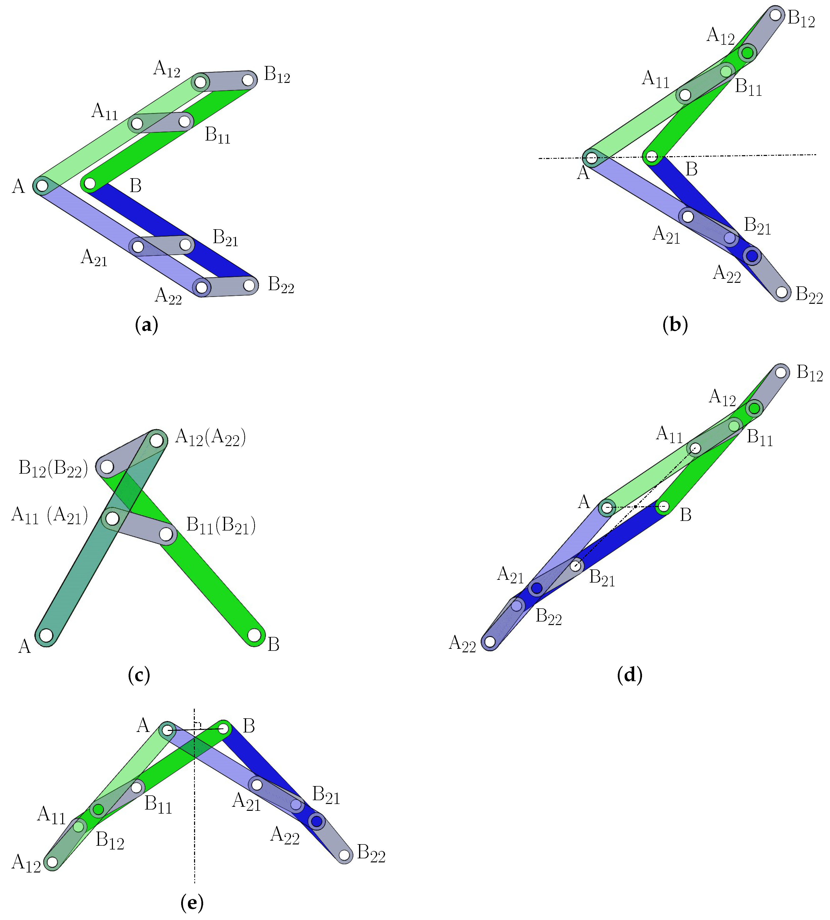
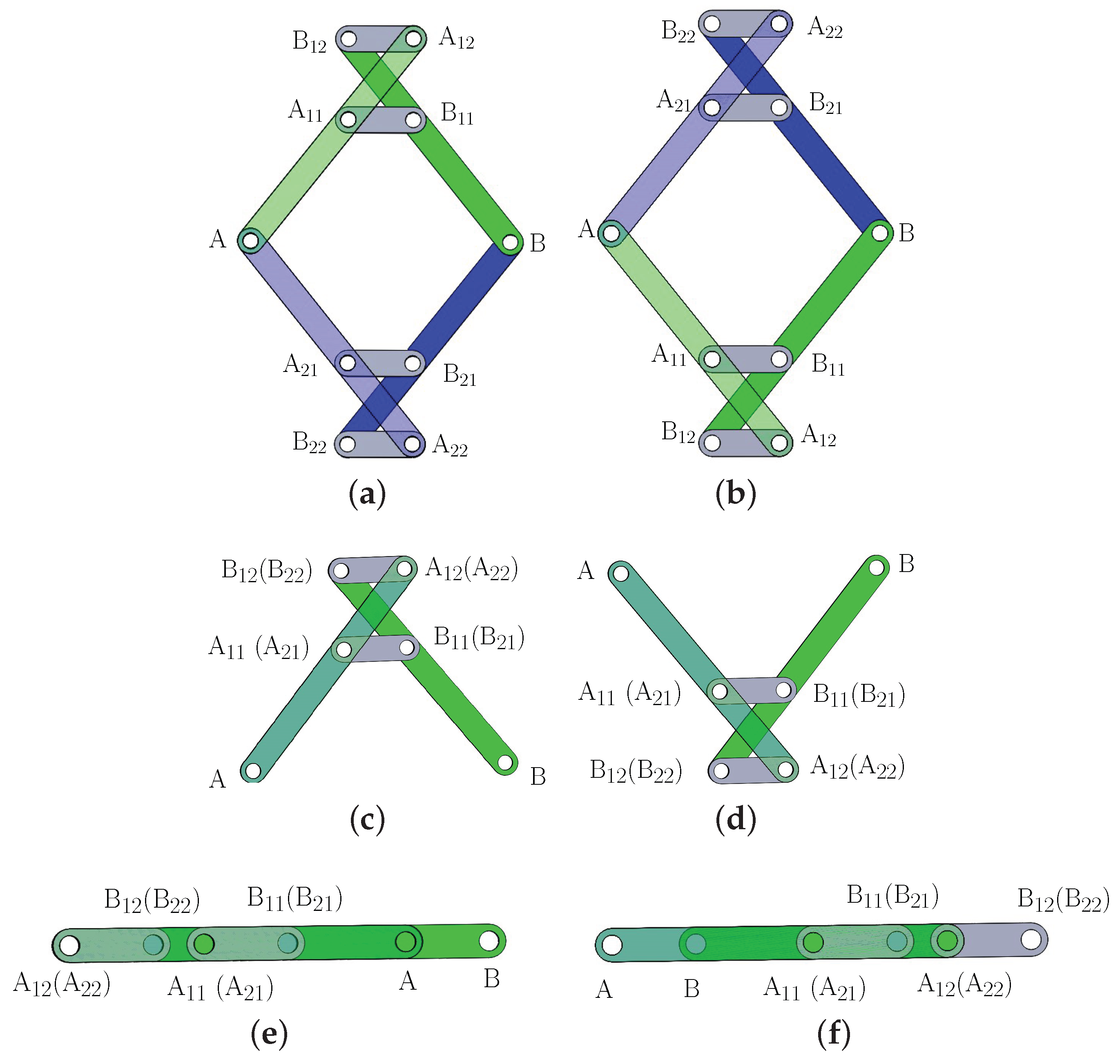
| 1 | 2 | L = 25 | Both closed-loop 4R sub-kinematic chains are parallelograms (Figure 2a). and are independent. |
| 2 | 1 | Both closed-loop 4R kinematic sub-chains are anti-parallelograms. The 8-link mechanism is symmetric about line (Figure 2b). | |
| 3 | 1 | Both closed-loop 4R sub-kinematic chains are anti-parallelograms that coincide with each other (Figure 2c), and the 8-link mechanism has two inactive joints A and B. | |
| 4 | 1 | Both closed-loop 4R kinematic sub-chains are anti-parallelograms. The 8-link mechanism is rotational symmetric (Figure 2d). | |
| 5 | 1 | Two closed-loop 4R sub-kinematic chains are anti-parallelograms. The 8-link mechanism is symmetric about the perpendicular bisector of (Figure 2e). |
| No | and (rad) | Description | Instantaneous DOF |
|---|---|---|---|
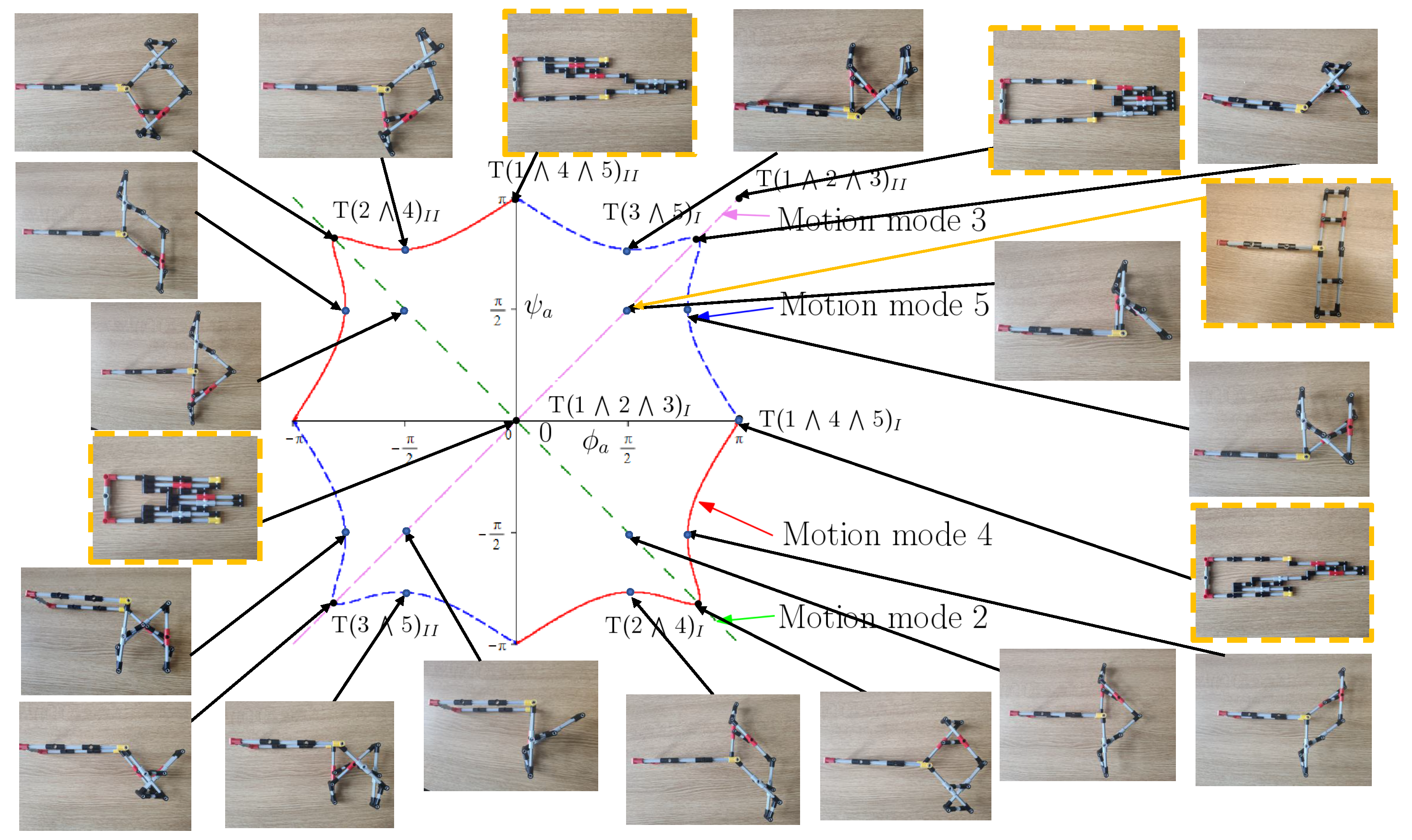
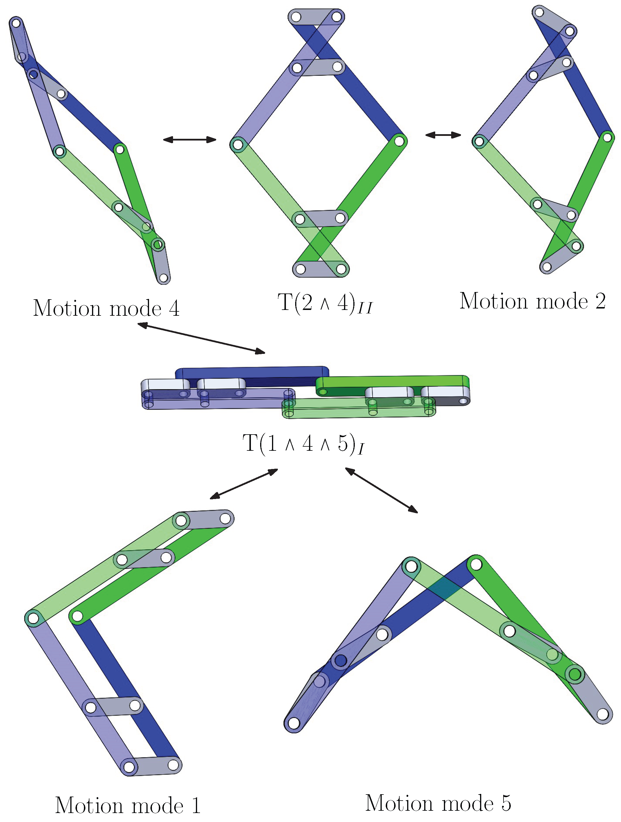
| T(2 ⋀ 4) | Links AB and BA are parallel to AB (Figure 5a). | 2 | |
| T(2 ⋀ 4) | Links AB and BA are parallel to AB (Figure 5b). | ||
| T(3 ⋀ 5) | Links AB and BA (i = 1 and 2) are parallel to AB (Figure 5c). | ||
| T(3 ⋀ 5) | Links AB and BA (i = 1 and 2) are parallel to AB (Figure 5d). | ||
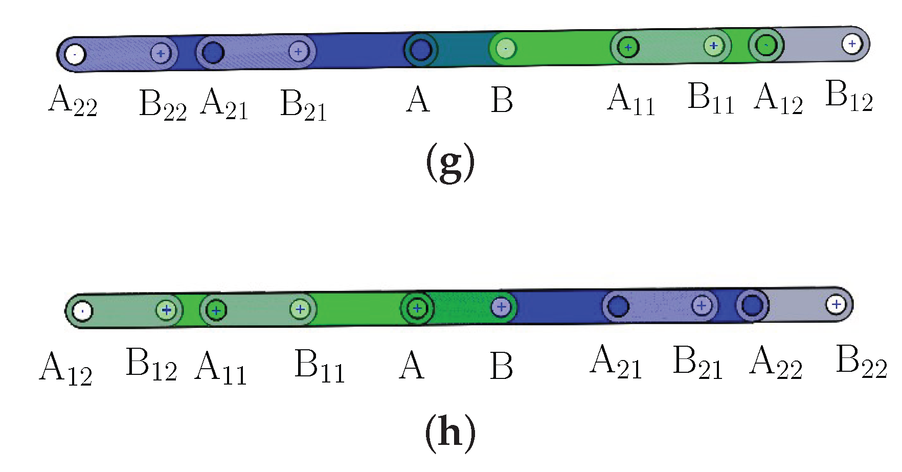
| T(1 ⋀ 2 ⋀ 3) | All the R joint centers are collinear (Figure 5e). | 4 | |
| T(1 ⋀ 2 ⋀ 3) | All the R joint centers are collinear (Figure 5f). | ||
| T(1 ⋀ 4 ⋀ 5) | All the R joint centers are collinear (Figure 5g). | ||
| T(1 ⋀ 4 ⋀ 5) | All the R joint centers are collinear (Figure 5h). |
Disclaimer/Publisher’s Note: The statements, opinions and data contained in all publications are solely those of the individual author(s) and contributor(s) and not of MDPI and/or the editor(s). MDPI and/or the editor(s) disclaim responsibility for any injury to people or property resulting from any ideas, methods, instructions or products referred to in the content. |
© 2023 by the authors. Licensee MDPI, Basel, Switzerland. This article is an open access article distributed under the terms and conditions of the Creative Commons Attribution (CC BY) license (https://creativecommons.org/licenses/by/4.0/).
Share and Cite
Kong, X.; Wang, J. Reconfiguration Analysis and Characteristics of a Novel 8-Link Variable-DOF Planar Mechanism with Five Motion Modes. Machines 2023, 11, 529. https://doi.org/10.3390/machines11050529
Kong X, Wang J. Reconfiguration Analysis and Characteristics of a Novel 8-Link Variable-DOF Planar Mechanism with Five Motion Modes. Machines. 2023; 11(5):529. https://doi.org/10.3390/machines11050529
Chicago/Turabian StyleKong, Xianwen, and Jieyu Wang. 2023. "Reconfiguration Analysis and Characteristics of a Novel 8-Link Variable-DOF Planar Mechanism with Five Motion Modes" Machines 11, no. 5: 529. https://doi.org/10.3390/machines11050529