Manipulator Trajectory Optimization Using Reinforcement Learning on a Reduced-Order Dynamic Model with Deep Neural Network Compensation

Abstract

This article reports the construction of an articulated manipulator’s hybrid dynamic model and trajectory planning and optimization of the manipulator using deep reinforcement learning (RL) on the dynamic model. The hybrid model was composed of a physical-based reduced-order dynamic model, linear friction and damping terms, and a deep neural network model to compensate for the nonlinear characteristics of the manipulator. The hybrid model then served as the digital twin of the manipulator for trajectory planning to optimize energy efficiency and operation speed by using RL while taking obstacle avoidance into consideration. The proposed strategy was simulated and experimentally validated. The energy consumption along paths was reduced and the speed was increased so the manipulator could achieve more efficient motion.

1. Introduction

The fourth industrial revolution is strongly promoted by governments around the world. Although industrial robots have already been widely deployed in factories for repetitive tasks, such as loading/unloading and pick-and-place, there are many tasks in factories that still require human operators. The use of manipulators is highly likely to increase, and the intelligence of the manipulator will therefore become increasingly important. For example, the smart and automatic generation of efficient or fast motion trajectories for a manipulator is needed. Trajectory planning has been an important issue for several decades because it strongly determines the effectiveness and cost of factory operations. Although the issue is classic, solutions continue to evolve due to the development of new technologies, such as artificial intelligence (AI). In the following section, related works on the trajectory optimization of robot arms are listed, including the traditional and the machine-learning methods.

The trajectory optimization of manipulators has been reported using the classic method, especially for energetic optimization. Singh and Leu used dynamic programming to optimize the trajectory to improve the energy efficiency and speed of one and two degrees of freedom (DOF) manipulators [1]. Field and Stepanenko adopted iterative dynamic programming for the trajectory energy optimization of a six-DOF industrial robot [2]. Hirakawa and Kawamura optimized the trajectory energy of a three-DOF robot arm using the cost function method [3]. Gregory et al. studied trajectory planning problems for a selective compliance articulated robot arm (SCARA) using an optimal control method [4]. Hansen et al. optimized the trajectory for an industrial robot; they considered a dynamic model of the robot, friction losses, and losses related to the servo and inverter [5]. Wigström et al. used a dynamic planning method to reduce the energy consumption of a robot arm by 10–20% [6]. Along with some works aiming for joint torque optimization [7,8], speed and time optimization are other popular targets. Sahar and Hollerbach used a graph search to optimize the time-minimum path for a two-DOF robot [9]. Gasparetto and Zanotto optimized a trajectory by considering the integral of jerk and execution time [10]. Rubio et al. proposed a computationally efficient algorithm to generate a time optimal and collision-free trajectory by evolving the trajectories in a discretization space and considering the physical constraints of industrial robots in industrial environments [11]. Ghasemi et al. translated the control problem into a nonlinear two-point boundary value problem to calculate the time-optimal trajectories of robot arms [12]. Schulman et al. developed trajectory optimization based on the sequential convex optimization procedure and efficient formulation of constraints to apply to various collision-free robot tasks in simulation [13]. On the other hand, some papers dealt with the control optimization for manipulators based on dynamic models. For instance, Krivošej and Šika actuated a three-DOF manipulator by the auxiliary cable mechanism and optimized the cable force distribution by using the simplex and genetic algorithm (GA) based on dynamic model analysis [14].

The typical trajectory optimization problem can also be approached by AI. Choi et al. proposed a two-phase learning algorithm to achieve global and local trajectory optimization and obstacle avoidance for more energy-efficient aircraft navigation [15]. Garg and Kumar used a GA and simulated annealing to find the optimal trajectory with minimum torque [16]. Tian and Collins used a GA to plan the trajectory with obstacle avoidance [17]. Števo et al. used the GA to optimize trajectory planning for an ABB robot arm [18]. Abu-Dakka et al. planned time-optimal trajectories for an industrial robot using an evolutionary algorithm [19]. Among research studies on AI, machine learning with deep neural network (DNN) models, aiding its versatility, has been utilized for the trajectory planning problem. Glasius et al. used the neural network method to generate trajectories with obstacle avoidance for a two-DOF robot arm [20]. Martín and Millán also utilized DNN to calculate the inverse kinematics for a robot manipulator, which enabled the robot to avoid obstacles [21]. Imajo et al. applied a recurrent neural network to generate obstacle-avoidance trajectories [22]. Levine et al. used deep learning for a robot arm to perform hand–eye coordinated grasping tasks [23]. Qiao et al. designed constraint equations for various physical limitations and self-collision avoidance for a mobile manipulator, defined the trajectory tracking as an optimization problem, and proposed the differential evolution algorithm to solve it [24].

To tackle the implicit relationship between the goal and complex dynamics, reinforcement learning (RL) has recently become a popular method in robotics [25] and task-oriented research. Stulp et al. used RL to generate motions for a robot manipulator for pick-and-place tasks [26]. Cheng and Zhang used deep reinforcement learning to develop obstacle avoidance control strategies and applied them to an unmanned marine vessel [27]. Cao et al. utilized Q-learning to construct a scalable and applicable method that can maximize the probability of arriving on time for vehicles in transportation systems [28]. For trajectory optimization, Kollar and Roy used RL for dynamic programming and a support vector machine to optimize the trajectory efficiency of robot campus exploration [29]. Akrour et al. developed a model-free trajectory optimization algorithm, which back-propagated a local Q-function, achieved a policy update in a closed form, and was deployed for two trajectory optimization tasks in simulations [30]. Li et al. used RL based on the path integral of dynamic movement primitive in joint space, and trained a manipulator with visual feedback to grasp objects under external perturbations [31]. Bucinskas et al. deployed online deep Q-learning to improve the positioning accuracy for an industrial manipulator with various operation times, speed, and load [32].

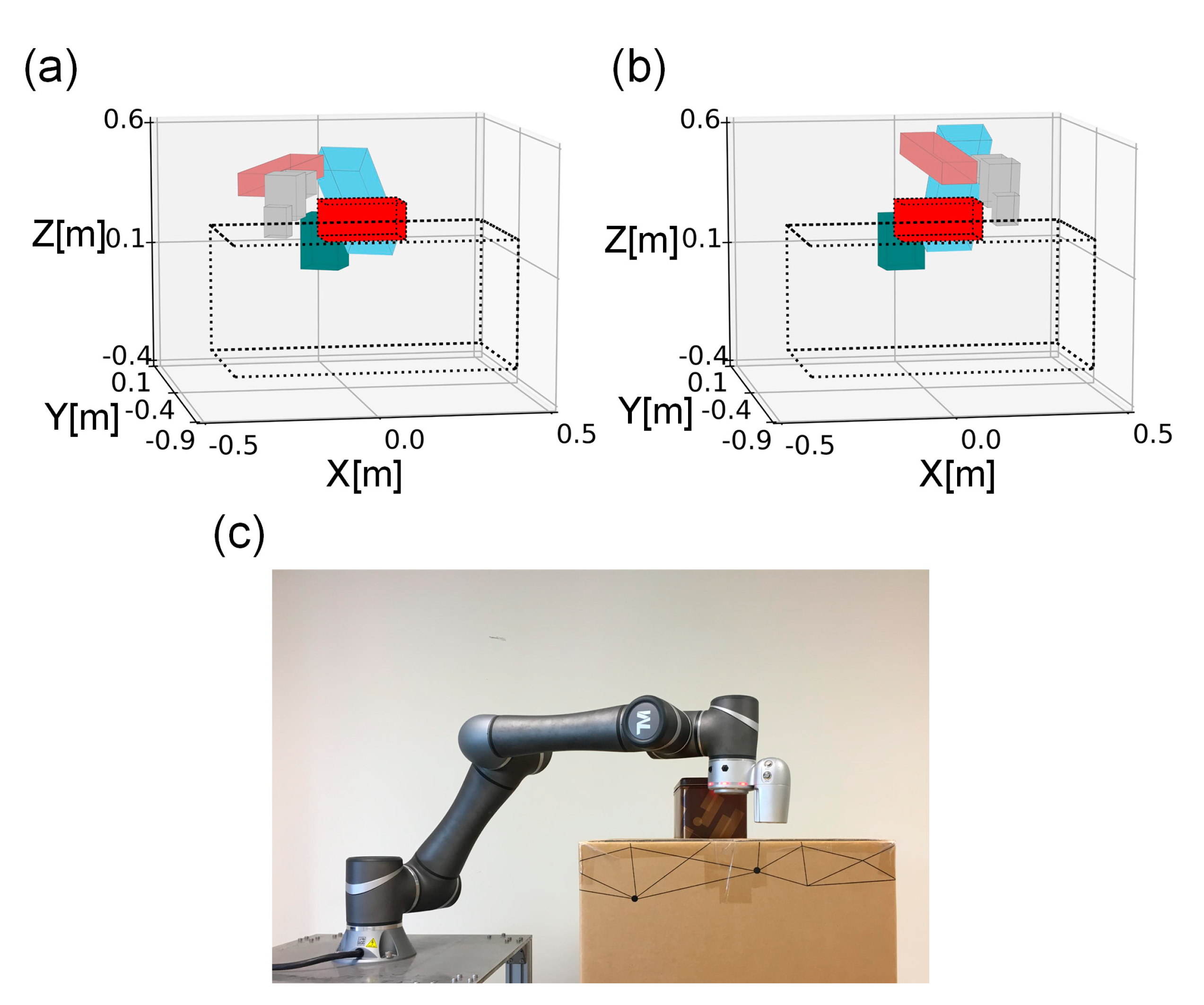
While the energy consumption of trajectory planning algorithms largely depends on the dynamic model of robot arms, the reported works rarely investigated physical models and trajectory optimization simultaneously. However, many industrial tasks require the precise estimation of the energy consumption and joint torque of the manipulator. For example, if a factory must use a manipulator to move very heavy loads, it needs to estimate and minimize energy consumption through trajectory optimization to save on electricity costs. In addition, the manipulator utilized in this paper was designed to carry sensors to examine patients lying in a hospital bed. More specifically, the proposed application is a postoperative free-flap registration and tracking system [33,34]. The goal of the application is to monitor the condition of the free flap on the face, head, or neck after surgery. The robot arm is set up beside the bed, and attached is an infrared camera and an RGB camera. The image system periodically calculates the condition of the free flap. The cameras need to keep a specific distance and angle from the free flap to obtain valid images, but the patient might move slightly or roll over unconsciously. Therefore, the image system will calculate where the cameras should be placed, and then the robot arm will move the cameras to that position. Some monitors or instruments placed around the bed to measure the patient’s health condition constitute obstacles, so the robot arm must avoid collisions with these objects. In such scenarios, the torque values of the manipulator should be precisely determined to meet medical safety standards and mitigate severe injuries that could result from accidents.

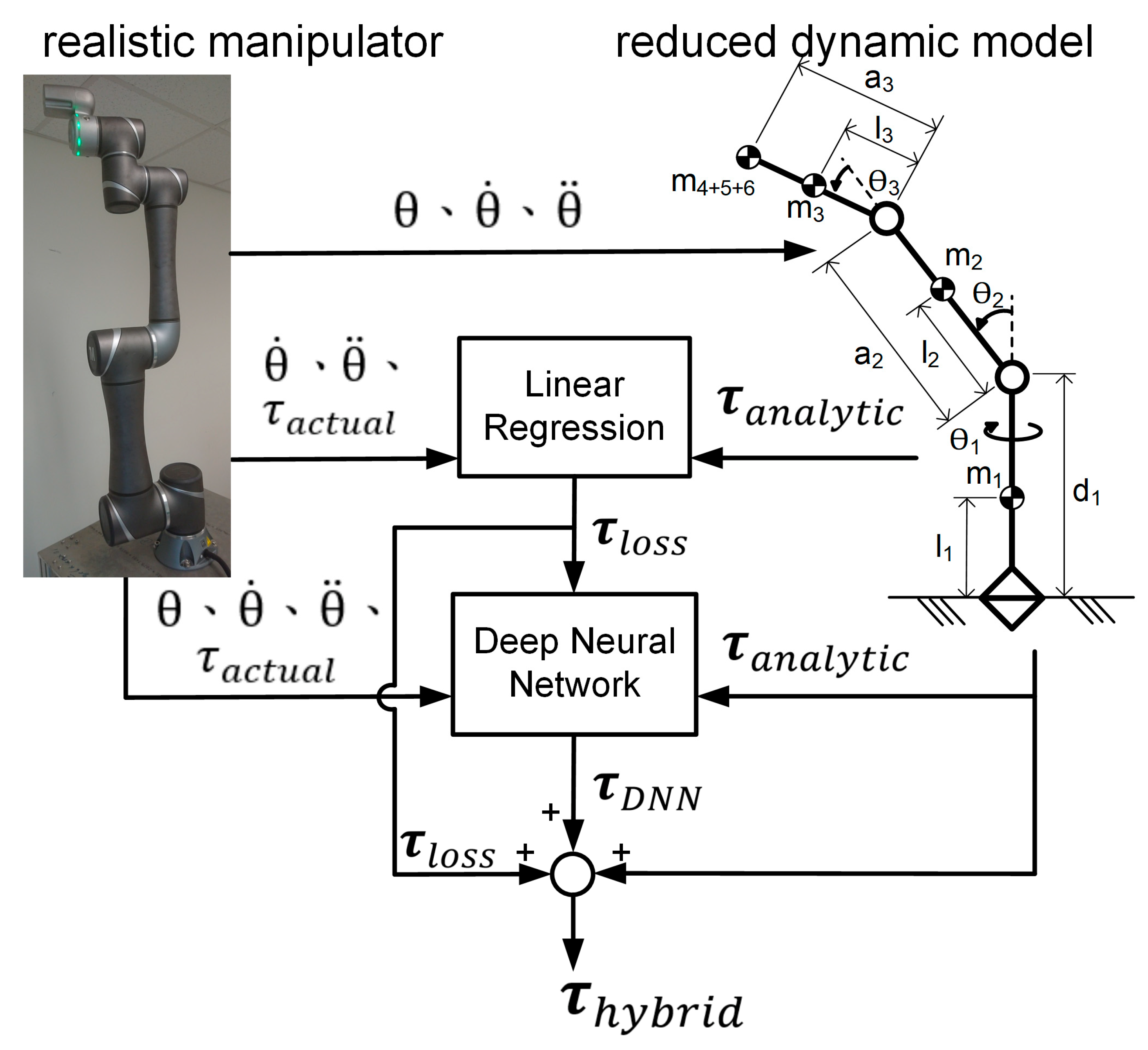
To precisely know the joint torques and calculate energy consumption, the precise dynamic model has to be figured out. Among research of robot arm dynamic model calibration, scarce reported work combined a physical-based model with a black-box (like DNN) model, while there exist many empirical factors in the dynamic model of manipulators other than analytic parts. For this paper, this approach was adopted, and the results are reported in two serial parts. The first is the development of a hybrid dynamic model, and the second is using the deep RL method to optimize the collision-free trajectory for energy and time consumption based on the developed dynamic model. The contributions are summarized as follows:

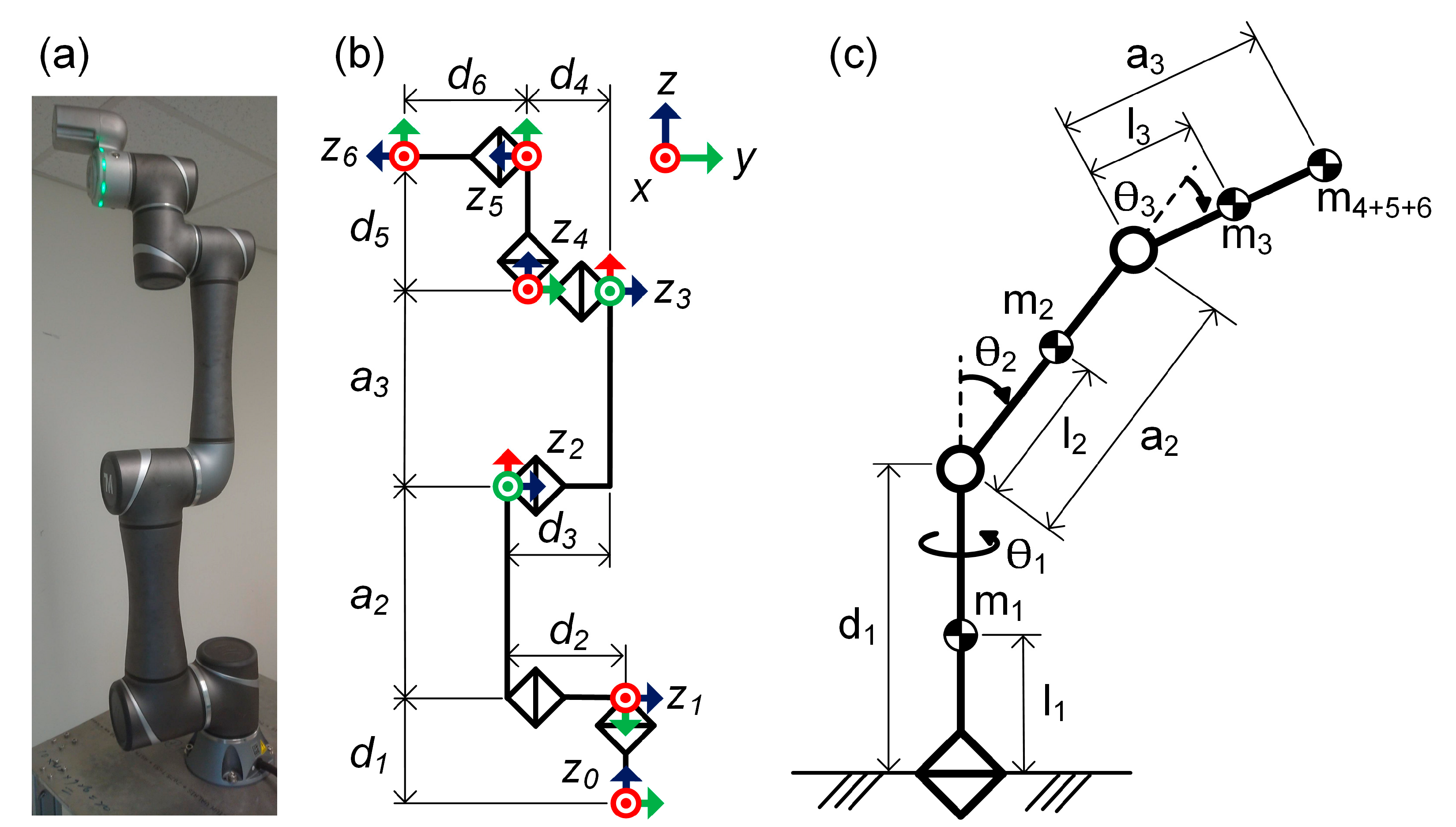
• A hybrid dynamic model of the manipulator was constructed, which was composed of an analytic three-DOF reduced-order dynamic model, linear non-idealized terms for mechanical energy loss, and a DNN model to calibrate other non-measurable and high-order empirical factors. While the hybrid model can largely decrease the computation complexity of the analytic model and reduce the training load and dataset size for DNN, it maintained high similarity to the real robot arm.
• To achieve energy efficiency with obstacle avoidance, the trajectory optimization of the manipulator was treated as a bandit problem. A trajectory planner initialized by a bi-directional rapidly-exploring random tree (Bi-RRT) and optimized by deep RL was introduced to spare complex mathematical deduction and calculations of the compound-goaled problem.
• Simulations and experiments were thoroughly conducted. In addition, performance comparisons to GA, human-taught trajectories, and the time compression method were executed as well. The results show that the proposed optimization method yields better performance.

The remainder of the paper is organized as follows. Section 2 describes the hybrid model and bounding box model of the manipulator, and Section 3 introduces the trajectory planning and optimization using RL. Section 4 reports the results of the simulation and experiments, and Section 5 concludes the work.

2. The Manipulator Models

The main method proposed in this paper is divided into two stages. First, the improved dynamic model of the manipulator was proposed by using the physical and data-driven sub-models. Then, the stateless deep reinforcement learning was utilized to optimize the trajectory and achieve obstacle avoidance based on the improved manipulator dynamic model. In this section, the construction of the hybrid dynamic model and the bounding box model for collision-free trajectory planning is demonstrated. Parameters were set according to those of the experimental validation platform, the six-DOF manipulator (TM5-900, Techman Robot, Inc., Taoyuan City, Taiwan), as shown in Figure 1a.

2.1. The Hybrid Dynamic Model of The Manipulator

The schematic diagram and the reduced-order dynamic model of the manipulator are shown in Figure 1b,c, respectively. The configuration design in Figure 1b is in contrast to the conventional industrial manipulator, which features a symmetrical mechanical design for dynamic balance. Furthermore, the last three DOFs intersect at a point to avoid singularity. Such a configuration, which supposedly offers more maneuverability, flexibility, and agility, is becoming increasingly common in modern collaborative robots, such as Sawyer [35], UR5e [36], and Panda [37]. The dynamics of the six-DOF articulated manipulator is approximated to a three-DOF reduced-order model to reduce the computation complexity. In more detail, in the general six-DOF dynamic model, the first and last three DOFs of the manipulator are mainly used for translational and rotational motions, respectively. To ease the process of solving the inverse kinematics, the axes of the last three DOFs in general design of articulated manipulators are intersected with one another, and the physical space of the manipulator that hosts these three DOFs (i.e., the waist) is usually compact and lightweight. Thus, when the manipulator performs tasks with an extended arm posture and large displacement, the rotational motion of the last three DOFs has little effect on the overall dynamics. Thus, the analysis of the overall six-DOF dynamics of the manipulator can be approximated by using a reduced-order three-DOF manipulator model that maintains the three translational DOFs and approximates the three rotational DOFs as a point mass mounted at the end of the third link. In this way, the computation cost of the reduced-order model is much lower than that of the original model, yet maintains the ability to extract the dynamic characteristics of the original manipulator. This approximation is achievable because the manipulator in general has less mass, a smaller size, and small motors that output less power in the last three joints compared to the first three DOFs. Thus, the manipulator’s energy consumption is mainly the result of the first three DOFs. Note that the mass and inertia effects of the last three DOFs with respect to the base frame are still maintained in the reduced-order model because the mass of the last three DOFs are preserved by the modeling of the joints as a point mass; only the rotational kinematic energy of the last three DOFs are ignored. This reduced-order model assumption restricts the solution to systems similar to the application proposed in [33,34], in which the author participated. The manipulator carries cameras at the endpoint and never changes the load during the task, so the last three joints could be considered a lump of mass. Meanwhile, the last joints do allow relatively small rotations during the task. In addition, the proposed algorithm can be extended to a six-DOF dynamic model as well, but the learning algorithm requires many more computational resources and a longer training time.

The hybrid dynamic model is composed of three sub-models:

$${\mathbf{\tau }}_{hybrid}={\mathbf{\tau }}_{analytic}+{\mathbf{\tau }}_{loss}+{\mathbf{\tau }}_{DNN}$$

(1)

where

$${\mathbf{\tau }}_{analytic}=\mathrm{M}\left(\mathbf{\theta }\right)\ddot{\mathbf{\theta }}+C\left(\mathbf{\theta },\dot{\mathbf{\theta }}\right)+\mathrm{G}\left(\mathbf{\theta }\right)$$

(2)

$${\mathbf{\tau }}_{loss}=B_m\ddot{\mathbf{\theta }}+C_m\dot{\mathbf{\theta }}+f_c\left(sign\left(\dot{\mathbf{\theta }}\right)\right)$$

(3)

$${\mathbf{\tau }}_{DNN}=DNN\left(\mathbf{\theta },\dot{\mathbf{\theta }},\ddot{\mathbf{\theta }}\right)$$

(4)

The vector $\mathbf{\theta }$ is the joint angles of the first three DOFs.

The first sub-model ${\mathbf{\tau }}_{analytic}$ represents the analytic reduced-order dynamic model of the manipulator. The model was derived using the Lagrangian method, and the symbols $\mathrm{M}\left(\mathbf{·}\right)$, $C\left(\mathbf{·}\right)$, and $\mathrm{G}\left(\mathbf{·}\right)$ represent the inertial, centrifugal and Coriolis, and gravitational terms, respectively. The derivation and the expanded form of the model are described in Appendix A. The values of the associated parameters are set according to those of the TM5-900.

The second sub-model ${\mathbf{\tau }}_{loss}$ compensates for the empirical energy loss caused by the mechanical transition system, including motor rotation, damping, and friction. The coefficients $B_m$, $C_m$, and $f_c$ are the motor inertia, the equivalent damping coefficient, and the dynamic friction coefficient, respectively. Because these coefficients are generally implicit and dependent on individuals, the linear regression method was utilized to determine the coefficient values by minimizing the difference between the torques of the dynamic model and the measured torques of the realistic manipulator ${\mathbf{\tau }}_{actual}$. That is:

$$\left[\begin{array}{ccc}{B}_m& C_m& f_c\end{array}\right]=[\ddot{\mathbf{\theta }}\hspace{1em}\dot{\mathbf{\theta }}\hspace{1em}sign(\dot{\mathbf{\theta }}\left){]}^{+}\right({\mathbf{\tau }}_{actual}-{\mathbf{\tau }}_{analytic})$$

(5)

where $+$ means pseudo inverse. The data on the right side were experimentally collected, and the experiment part is described in Section 4.1.

In addition to the two sub-models based on physical dynamics, the sub-model ${\mathbf{\tau }}_{DNN}$ based on DNN was added to cover other nonlinear and higher-order dynamic behaviors of the manipulator, such as lubricant viscosity in the bearings, the dead zone of motor activation, and static friction. The DNN overweighs other methods for such nonlinear and arcane problems, and it can run faster with suitable equipment. The DNN model was trained using supervised learning. The inputs of the model include angle $\mathbf{\theta }$, velocity $\dot{\mathbf{\theta }}$, and acceleration $\ddot{\mathbf{\theta }}$ of the first three joints of the manipulator. The labeled outputs of the model are the residual torques ${\mathbf{\tau }}_{residual}$ between the torques of the manipulator ${\mathbf{\tau }}_{actual}$ and the torques of the physical models ${\mathbf{\tau }}_{analytic}+{\mathbf{\tau }}_{loss}$. The ${\widehat{\mathbf{\tau }}}_{residual}$ represents the estimates of the DNN model after training.

$$\left\{\begin{array}{l}{\mathbf{\tau }}_{actual}-\left({\mathbf{\tau }}_{analytic}+{\mathbf{\tau }}_{loss}\right)={\mathbf{\tau }}_{residual}\\ {\mathbf{\tau }}_{DNN}=DNN\left(\mathbf{\theta },\dot{\mathbf{\theta }},\ddot{\mathbf{\theta }}\right)={\widehat{\mathbf{\tau }}}_{residual} \end{array}\right.$$

(6)

The DNN model has five hidden layers, with 256, 512, 1024, 512, and 256 neurons in each layer, respectively. The activation functions in the hidden layers are tanh, and those of the output layer are linear. These hyper-parameters and model structures were determined by heuristics and experience. During the training process, the dropout rate of each hidden layer was set to 0.5, and the Adam optimizer was utilized to minimize the mean square error between the actual torque and the torque value generated from the DNN model.

Figure 2 depicts the overall construction flow of the hybrid dynamic model. First, the three-DOF analytic reduced-order dynamic model was constructed given the mechanical parameters of the manipulator from the manufacturer. Then, the joint states $\left(\mathbf{\theta },\dot{\mathbf{\theta }},\ddot{\mathbf{\theta }}\right)$ and the torques ${\mathbf{\tau }}_{actual}$ of the manipulator at each instant during motion were collected. The torques of the analytic model ${\mathbf{\tau }}_{analytic}$ were correspondingly computed using Equation (2). The time-series of ${\mathbf{\tau }}_{actual}$ and ${\mathbf{\tau }}_{analytic}$ were utilized to calculate the coefficients in Equation (3) by using Equation (5). Then, given the time series of joint states $\left(\mathbf{\theta },\dot{\mathbf{\theta }},\ddot{\mathbf{\theta }}\right)$, the torques of the loss model ${\mathbf{\tau }}_{loss}$ were computed by using Equation (3). Next, the time series of $\left(\mathbf{\theta },\dot{\mathbf{\theta }},\ddot{\mathbf{\theta }}\right)$, ${\mathbf{\tau }}_{actual}$, ${\mathbf{\tau }}_{analytic}$, and ${\mathbf{\tau }}_{loss}$ were utilized to train the DNN model using Equation (6). Finally, the hybrid dynamic model was constructed, as shown in Equation (1).

2.2. The Bounding Box Model and Singularity Penalty

To generate collision-free motion trajectories, the actual geometric shape of the manipulator and obstacles should be considered; however, the actual shape of each manipulator link is too complicated to calculate collision in a reasonable time. Thus, oriented bounding box techniques [38] were utilized.

Each object in the simulation environment, including the manipulator links and surrounding obstacles, was enclosed by a compact oriented rectangular bounding box. The separating axis theorem (SAT) [39] was then applied to check for dynamic collisions between any two bounding boxes [40]. In the three-dimensional case, if there was no collision of two cuboids, such as bounding boxes A and B for example, there was at least one separating plane between them. In considering the planes spanning two edges of the two boxes and the planes spanning two edges of the same box, there are three axes that constitute the face normal from A and three axes as the face normal from B. Furthermore, there are nine axes from all the pairs of edges of A and B, with Edge 1 of A crossing Edge 1 of B, Edge 1 of A crossing Edge 2 of B, Edge 2 of A crossing Edge 1 of B, and so on. Therefore, there were a total of $3+3+9=15$ possible separating planes and axes that should be checked. The flow chart showing self-collision detection is shown in Figure 3.

In the empirical implementation, the position and orientation of each link along with the bounding box can be derived in real time using forward kinematics with known joint angles. The position and orientation of other static or moving obstacles should be predefined or detected using other sensory systems. Once the status of all the objects is known, the link-to-link or link-to-obstacle collisions can be detected. Figure 4 illustrates a simulation environment, where the manipulator and obstacles are covered by the bounding boxes ready to check the collision status.

Notice that the process to deal with singularities of the manipulator is similar to that for collision avoidance. When a singularity happens, a penalty score will be given so that the learning process knows that it is not a good trajectory. In addition, no other restrictions are placed for the lumped joints because the joints are fixed, and they also have separated bounding boxes when calculating the collision.

3. Trajectory Optimization by Reinforcement Learning

After the model was constructed and the collision avoidance strategy was set up, the next step was trajectory optimization for energy efficiency or motion speed, which improves the performance of the manipulator in an empirical factory utilization.

The general motion trajectory of the manipulator is composed of key positions, including a start point, via points, and an end point. While the start and end points are usually known a priori, the variation of the trajectory lies in the position and time stamp of the via points, which are the optimization variables. In between the start, via, and end points, a cubic spline trajectory was adopted [41]. The speed limitation of the first three joints of the manipulator was also considered and set to $180 \left[\mathrm{deg}/\sec \right]$ according to the manipulator’s operation manual [42]. In this case, a smooth trajectory (i.e., position and velocity continuity) prevents the manipulator from wasting energy with abrupt motions that easily reach joint torque limits; thus, the generated trajectory can be optimized for the overall motion requirement, but it is not constrained by undesired abrupt movements.

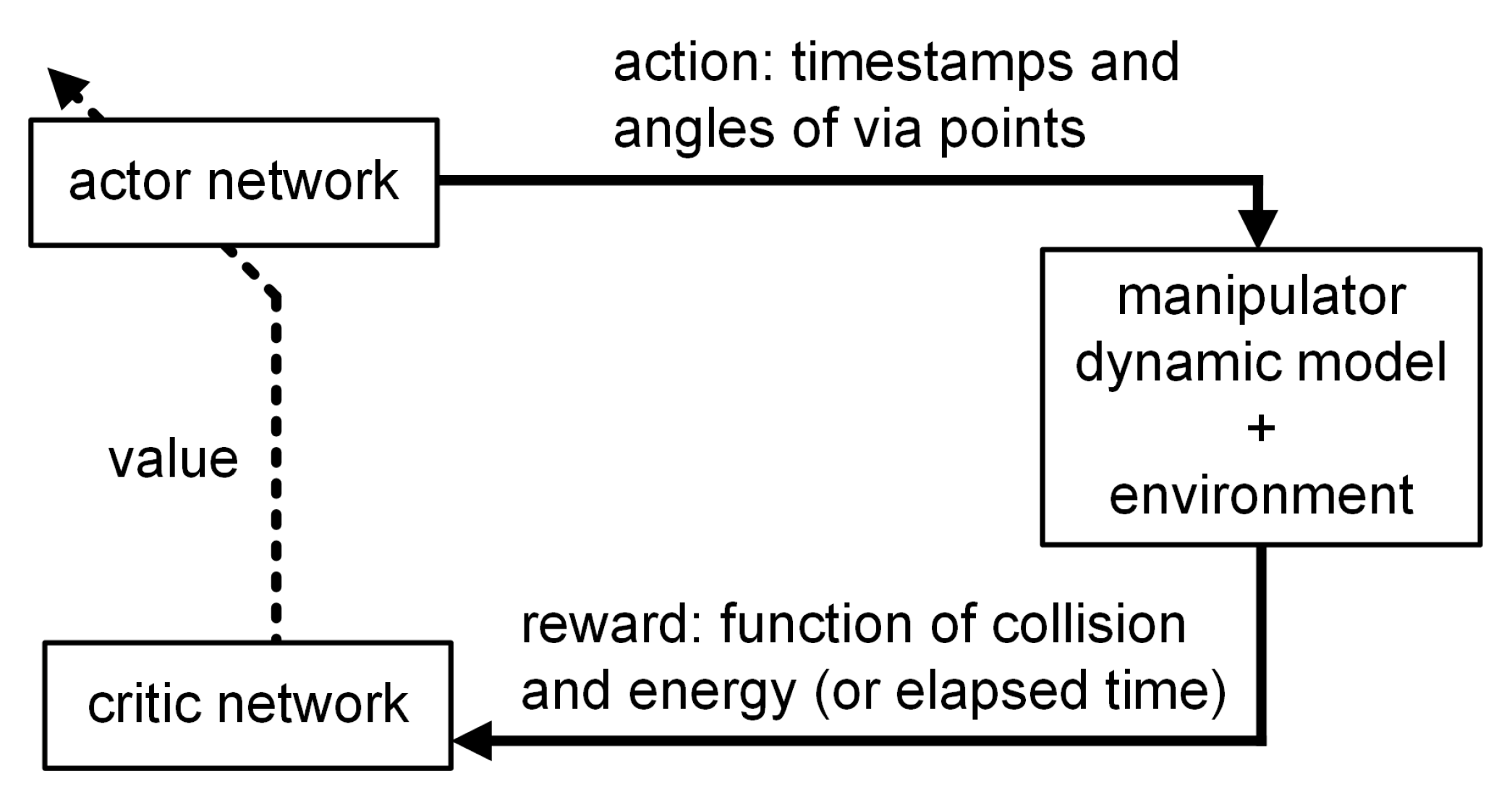
Deep reinforcement learning was utilized for trajectory optimization because it can spare complicated constraint setting and analytics while achieving comparably good results, which is user-friendly for industrial users. The algorithm used here was proximal policy optimization (PPO), proposed by OpenAI in 2017 [43]. The PPO is based on the actor-critic structure. The actor, which is gradually optimized regarding its performance during the training process, takes actions by changing the positions or time stamps of via points in this case. This is followed by the critic, which gives the actor a score according to the action it takes and guides the actor to change its action to achieve a higher score. The reward here was set for energy or speed optimization, and the reward of the trajectory was higher if its energy consumption or elapsed time was lower. Different trajectories have different rewards, and the trajectory with the highest reward is the desired one. The actor-critic structure in PPO is illustrated in Figure 5.

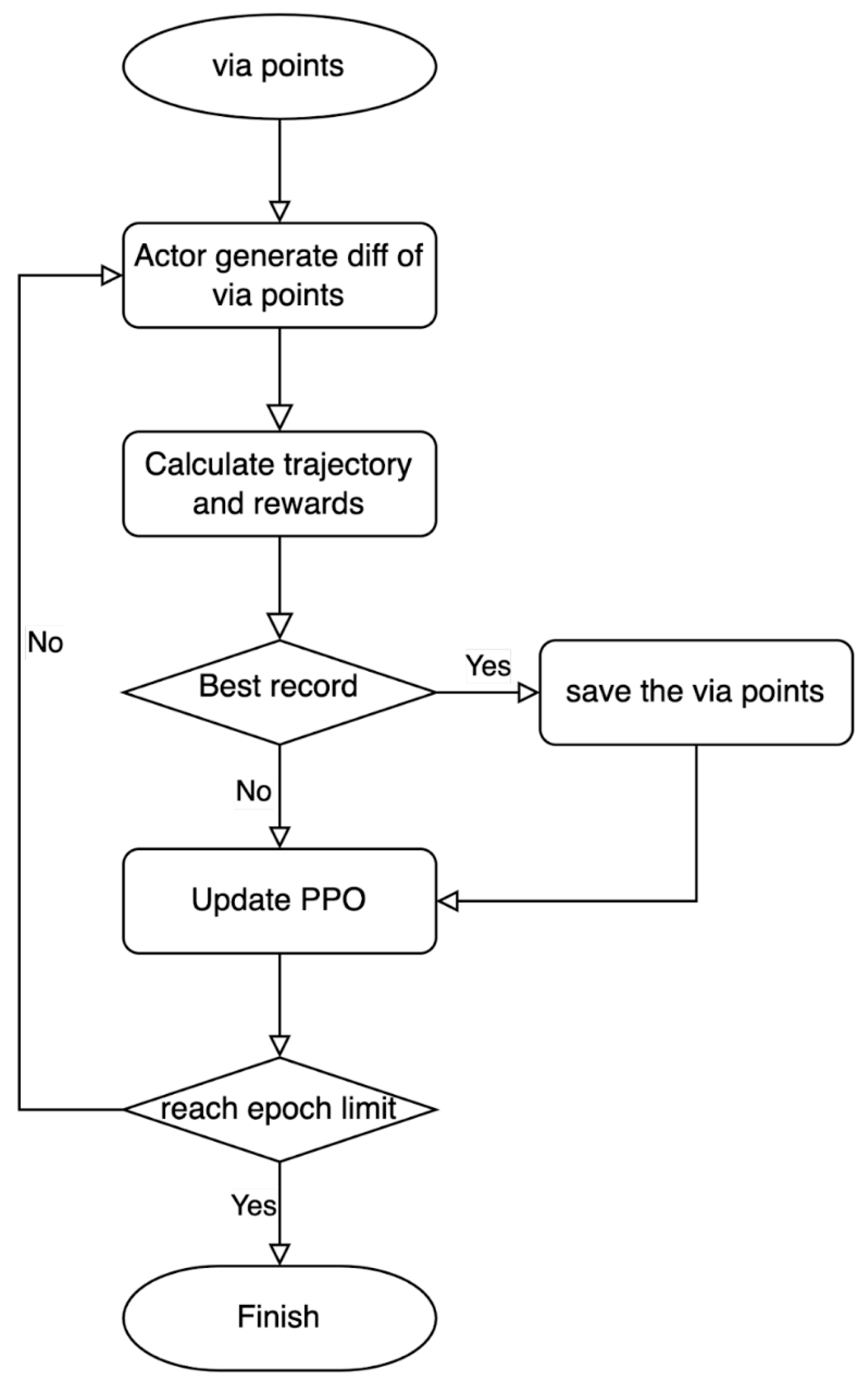
The optimization was treated as a bandit problem or a stateless problem since the arrangement of object position in industrial factories changes once in a long time; therefore, the state, containing the start point, end point, and obstacles, almost maintains constant. The classic RL problem generates action data corresponding to various state data. In contrast, each case of the trajectory planning was trained and optimized separately without any state data inputting to the DNN. During this process, it is not necessary to consider transition models as well. In the actor space, the algorithm adjusted the positions of the via points for energy optimization or adjusted the timestamps of the via points for speed optimization. Then, the value function was updated by collecting action and reward data. Finally, the data were used to update the parameters of the actor and the critic.

The DNN models in the learning algorithm contain an actor network and a critic network. There is no input layer in the networks. Although they were tuned slightly using heuristics, the following network configurations referenced the model structure in the original PPO paper [43]. The two networks both have two fully-connected hidden layers based on rectified linear unit (ReLU) neurons. Both networks have 512 neurons in the first layer and 256 neurons in the second layer. The critic network only has one neuron in the output layer, and the action data from the actor network contain angles of the first three manipulator joints for all via points. The output layer of the actor network parallel includes the mean layer μ and the covariance layer σ, both as the same dimensions as the number of action data, passing through a Gaussian probability function to increase exploration when training [44]. In this study, RL was used to solve this optimization problem, and the goal was to find the best via points connected by cubic equations. That is, once the via points were determined, the trajectory was also determined. As shown in Figure 5, the action output from the actor network led to adjustments to the via points, and the reward given back by the dynamic model considered the collision and energy consumption. Here, the principle was that the more serious the collision was, the more negative the reward would be; if there was no collision, less total energy consumed by the entire trajectory could obtain a more positive reward. The total algorithm to optimize the via points based on PPO is depicted in Figure 6.

3.1. Determination of The Initial Via Points

If there is no obstacle, the determination of the initial via points is not critical because the follow-up optimization will adjust the position and time stamp of the via points. In contrast, when obstacles do exist, the initially selected via points should be outside and away from the obstacles to speed the optimization convergence. The bi-directional rapidly-exploring random tree (Bi-RRT) [45] was utilized to find the initial via points.

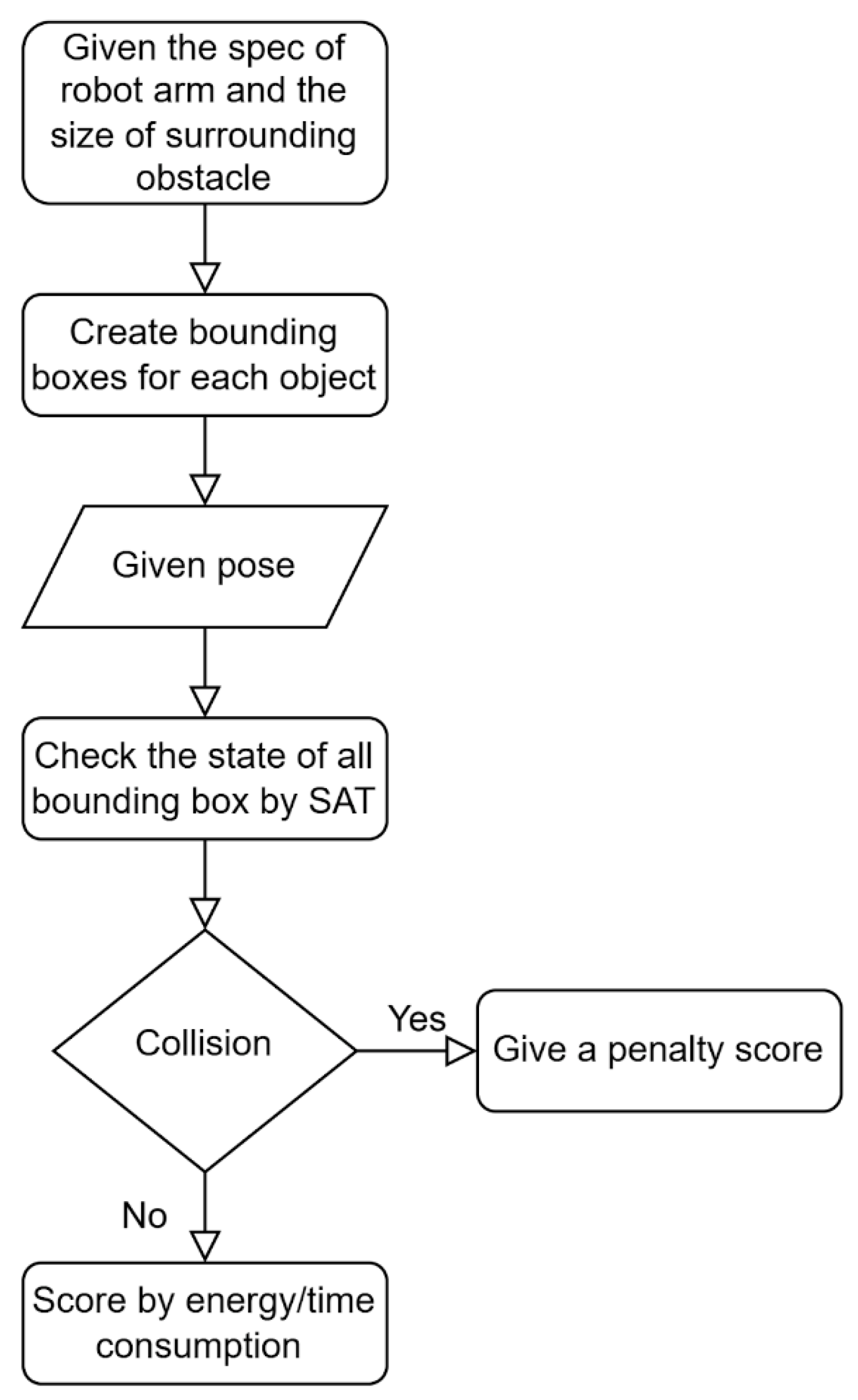
The details of the implementation of the Bi-RRT are described as follows. First, the physical spaces taken by the manipulator and the obstacles were modeled as bounding boxes, as described in Section 2.2, which were to be avoided by the Bi-RRT. Second, points on the midplane were selected as goals for the Bi-RRT to search from the start and end points. The midplane was defined as the plane that was normal to and intersected with the midpoint of the line segment between the start and end points. Third, the convex hull formed by the projected vertices of the obstacles on the midplane was computed. Then, eight points with an equal angular distribution (i.e., ${45}^{°}$ apart) and on the boundary of the convex hull were chosen as the initial via points. In addition, the midpoint of the line segment between the start and end points was chosen. Finally, the Bi-RRT was utilized to find collision-free paths that connected the start and end points to the eight goal points, i.e., at most nine Bi-RRT paths if all searches were successful.

Because the nodes generated by the Bi-RRT were determined by the length of each search step, not all the nodes should be the initial via points, and the node was removed if the path without it was shorter and still collision-free. The nodes from the start point were sequentially and individually checked and iterated until no node could be removed. The remaining nodes were set as the initial via points.

3.2. Energy Optimization

For energy optimization, the reward was set as:

$$rewar{d}_E=\left\{\begin{array}{c}-\frac{1}{dis{t}_{min}} , if collision detected\\ \frac{{10}^4}{\sum Energy} , if collision free\end{array}\right.$$

(7)

The symbol $dis{t}_{min}$ indicates the minimum distance between the two nearest bounding boxes in the whole trajectory. The symbol $\sum Energy$ is the total energy consumption of the model, which is defined as:

$$\sum Energy={{\displaystyle \sum }}_{j=1}^3{{\displaystyle \int }}_{t_i=0}^{t_f=t}{\tau }_j\left(t\right){\dot{\theta }}_j\left(t\right)dt$$

(8)

where $\left[t_i{t}_f\right]$ are the start and final time stamps of the trajectory, and $\left({\tau }_j,{\theta }_j\right)$ are the j^th joint torque and joint angle, respectively. The main idea of the reward setting shown in Equation (7) is that if the collision occurs, then the reward is negative, and the reward is lower if the collision is more severe. In contrast, if there is no collision, the reward is positive, and the score is higher when the energy consumption is lower. Equation (7) can be utilized regardless of the number of obstacles.

3.3. Speed Optimization

The speed optimization process is similar to the energy optimization process, but the goal is to reduce the elapsed time from the start point to the end point while avoiding an overloaded operation. The reward was set as:

$$rewar{d}_S=\left\{\begin{array}{c}-\left|{\tau }_{limit}-{\tau }_{peak}\right|, if torque over limit\\ {10}^3\times tim{e}_{reduction}, otherwise\end{array}\right.$$

(9)

where $tim{e}_{\mathrm{reduction}}$ is the difference of time consumption before and after optimization. The main idea of the reward setting shown in Equation (9) is that if the computed torque exceeds the limit, the reward is negative, and the more the torque exceeds, the lower the reward. In contrast, the reward is positive and higher if the time reduction is more significant.

Note that the energy-optimized trajectory was utilized as the initial trajectory for speed optimization because it is collision-free, and the motion profile is relatively smooth. In this case, the optimization aims at maintaining the same profile while increasing the magnitudes of the motion states and torques until the manipulator achieves its torque limit [46,47]. In this work, the energy and speed optimizations were executed separately because the optimization of these two goals is generally oriented toward different optimized sets. Therefore, rather than using a reward composed of both energy consumption and speed objectives, energy and speed were optimized separately with different reward functions.

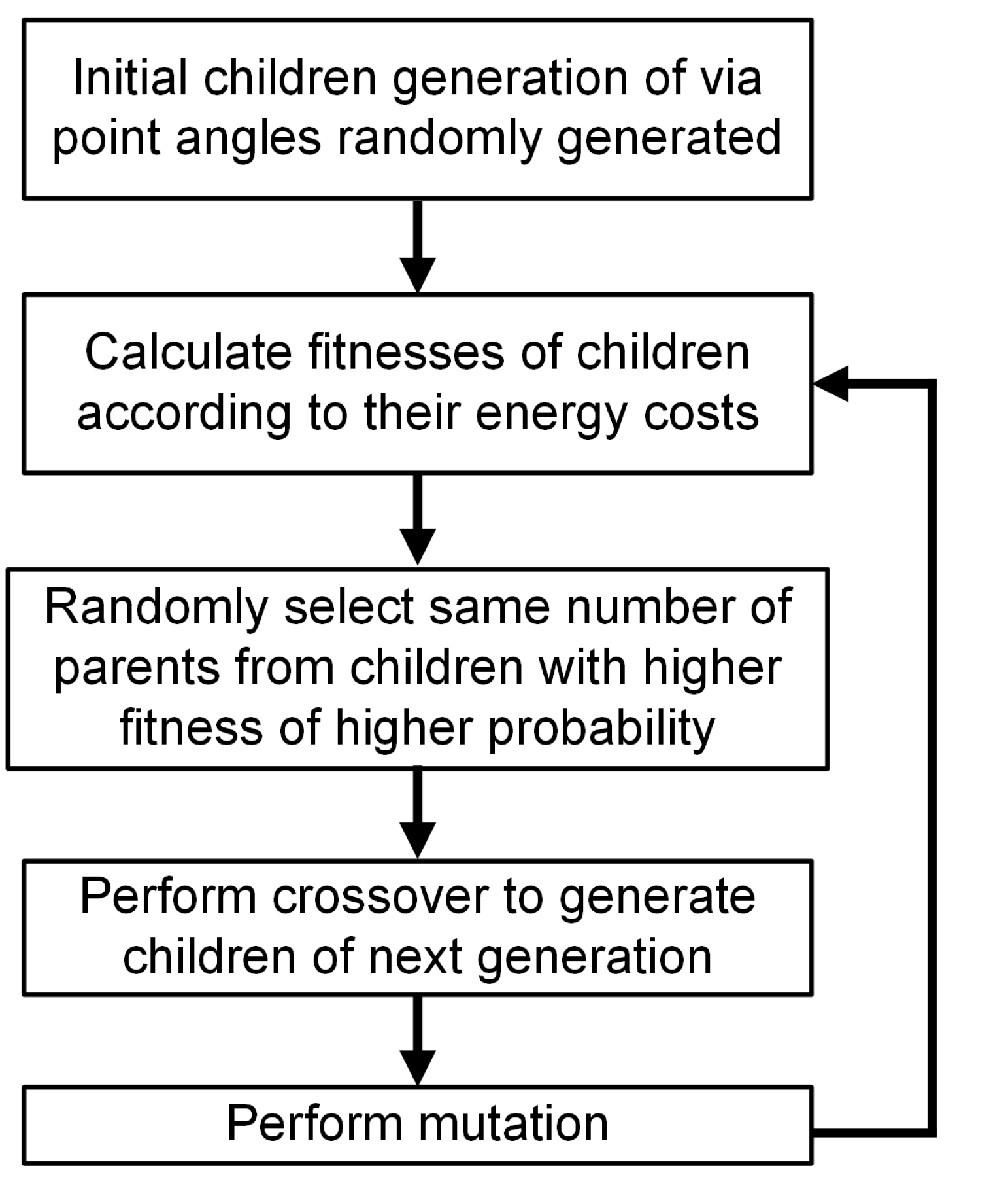
3.4. Genetic Algorithm

Furthermore, to compare the performance of the proposed method with classic artificial intelligence methods, GA was adopted for evaluation as well. GA mimics natural genetic exchange rules and follows the idea of the “survival of the fittest” to generate increasingly better offspring over several generations. In each generation loop, a set of children, of which each consists of six lines of binary values as genes, would first be converted to decimal values as six via angles, and the energy cost based on Equation (8) would be calculated corresponding to each child. Then, the same number of children would be randomly selected as parents of the next generation in the children set, following the rule that the child with a lower energy cost was assigned a higher probability to be chosen.

After that, each parent would have a high probability to exchange some of their binary elements with one of the children (selected randomly) at random element places, generating offspring as the next generation. Through the process, parents with a lower energy cost would generate more offspring, and finally the optimal set of via angles would appear in the last generation. The illustration depicting the GA procedure is shown in Figure 7.

4. Simulation and Experiment Results

In this section, the experiment results related to the hybrid dynamic model described in Section 2 are first demonstrated. Then, the simulation and experiment results related to the trajectory optimization described in Section 3 are reported.

4.1. Performance of The Hybrid Dynamic Model

The construction of the hybrid dynamic model requires measurements of various states of the manipulator as described in Section 2, including joint angles, velocities, accelerations, and torques. Due to the necessity for motion data (i.e., velocity and acceleration), it was efficient to collect the required data while the manipulator was moving according to preset trajectories containing variations of joint orientation, velocity, and acceleration. The trajectories were randomly chosen within the robot’s workspace, and the trajectories were set bidirectionally and with various speeds to cover a wide range of joint motions. Figure 8a,b, drawn using Python and Matplotlib, show the training trajectory data groups, T1 and T2, each with five trajectories. The collected data at each instant (i.e., time stamp) were considered as one data set, and each trajectory contained 50 to 150 data sets. In total, 10,306 data sets were collected, of which 70% and 30% were used for training and validation in the DNN model training, respectively. The model was trained for 100 epochs, and the loss stabilized after the 15th epoch.

The performance of the DNN sub-model was evaluated using the ten different trajectories, as shown in Figure 8c,d drawn using Python and Matplotlib. The means and standard deviations (STD) of the energy errors between the dynamic model and the manipulator were utilized for comparison, and the experiment results are shown in

Table 1. The energy consumption discrepancy between the empirical manipulator and the models with different compensation terms.

	Error [J]	Joint 1	Joint 2	Joint 3	Total
${\tau }_{analytic}$	mean	$-$18.20	$-$2.32	$-$1.67	$-$22.20
	STD	8.89	5.13	10.10	14.00
${\tau }_{analytic}+{\tau }_{loss}$	mean	0.00	$-$0.70	$-$1.28	$-$2.09
	STD	1.09	1.13	0.97	1.76
${\tau }_{hybrid}$	mean	$-$0.03	$-$0.22	0.02	$-$0.23
	STD	0.87	1.01	0.48	1.42

. Three scenarios were compared: the analytic reduced-order model without any fitting (i.e., ${\tau }_{analytic}$), the analytic model with energy compensation (i.e., ${\tau }_{analytic}+{\tau }_{loss}$), and the hybrid dynamic model with energy compensation and the DNN model (i.e., ${\tau }_{hybrid}={\tau }_{analytic}+{\tau }_{loss}+{\tau }_{DNN}$). Using ${\tau }_{analytic}$ as the baseline, the averaged energy error of Joints 1 to 3 of the model ${\tau }_{analytic}+{\tau }_{loss}$ conceivably reduced by 100%, 69.8%, and 23.4%, respectively, and the overall energy error was reduced by 90.6%. The reduction of Joint 1 is most significant, because the joint supports the heaviest weight and inertia of the manipulator, so it ameliorates the most by ${\tau }_{loss}$. Next, with the added DNN term, the averaged energy error of Joints 2 and 3 of the complete model further decreased by 68.6% and 98.4%, respectively. The overall energy error was further reduced by 89.0%. In short, both the loss model and the DNN model significantly improved the accuracy of the dynamic model of the manipulator.

Furthermore, to examine the influence of the quantity of training data sets on the performance of the DNN model, the training and evaluating trajectory data groups, T1, T2, E1, and E2, shown in Figure 4, were separately utilized. Figure 9, drawn using Python and Matplotlib, depicts the errors of the manipulator energy consumption ($E_{error}$) and the root mean square errors (RMSE) of the joint torques (${\tau }_{RMSE}$) between the manipulator and the dynamic model. The results show that the model trained by a larger training set, T1+T2, has smaller total energy error means and STDs than those trained by a smaller set, T1 or T2, because the larger data set covers a larger variation for training. This also can be roughly observed in the RMSE of torques. There is no obvious trend to make conclusions among different evaluation data sets.

In this work, the DNN training process did not include variations in payload, but the experiments did evaluate the manipulator with various payloads. The results are shown in

Table 2. The energy consumption discrepancy and joint root mean square error (RMSE) torque between the empirical manipulator and the models with different payloads.

Error	Payload	516 gw			1029 gw			1544 gw
		${\mathit{\tau }}_{\mathit{a}\mathit{n}\mathit{a}\mathit{l}\mathit{y}\mathit{t}\mathit{i}\mathit{c}}$	${\mathit{\tau }}_{\mathit{a}\mathit{n}\mathit{a}\mathit{l}\mathit{y}\mathit{t}\mathit{i}\mathit{c}}+{\mathit{\tau }}_{\mathit{l}\mathit{o}\mathit{s}\mathit{s}}$	${\mathit{\tau }}_{\mathit{h}\mathit{y}\mathit{b}\mathit{r}\mathit{i}\mathit{d}}$	${\mathit{\tau }}_{\mathit{a}\mathit{n}\mathit{a}\mathit{l}\mathit{y}\mathit{t}\mathit{i}\mathit{c}}$	${\mathit{\tau }}_{\mathit{a}\mathit{n}\mathit{a}\mathit{l}\mathit{y}\mathit{t}\mathit{i}\mathit{c}}+{\mathit{\tau }}_{\mathit{l}\mathit{o}\mathit{s}\mathit{s}}$	${\mathit{\tau }}_{\mathit{h}\mathit{y}\mathit{b}\mathit{r}\mathit{i}\mathit{d}}$	${\mathit{\tau }}_{\mathit{a}\mathit{n}\mathit{a}\mathit{l}\mathit{y}\mathit{t}\mathit{i}\mathit{c}}$	${\mathit{\tau }}_{\mathit{a}\mathit{n}\mathit{a}\mathit{l}\mathit{y}\mathit{t}\mathit{i}\mathit{c}}+{\mathit{\tau }}_{\mathit{l}\mathit{o}\mathit{s}\mathit{s}}$	${\mathit{\tau }}_{\mathit{h}\mathit{y}\mathit{b}\mathit{r}\mathit{i}\mathit{d}}$
$E_{error}$ [J]	mean	$-$18.60	$-$5.54	$-$1.98	$-$19.50	$-$6.54	$-$2.96	$-$19.70	$-$6.89	$-$3.31
	STD	5.62	2.44	0.93	5.54	2.69	1.17	5.21	3.11	1.54
${\tau }_{RMSE}$ [Nm]	mean	10.50	5.01	4.21	10.90	5.43	4.48	11.10	5.72	4.68
	STD	1.00	1.28	0.35	1.15	1.43	0.47	1.29	1.58	0.51

. The similarity of the results across tests with different payloads indicates that no matter how the payload increases, the added sub-models, ${\tau }_{loss}$ and ${\tau }_{DNN}$, can reduce the energy and torque errors. This further indicates that the regression and the DNN training process successfully learned the intrinsic mechanical and dynamic characteristics of the manipulator rather than overfitting to the characteristics of free motion without any payload. The results also show that as the payload increases, the errors also increase, which indicates that the payloads do affect the dynamic model. If the payloads are known a priori, the motion of the manipulator subjected to these specific payloads can be included in the DNN model training to improve model accuracy.

4.2. Simulation Results of Trajectory Optimization

Before the empirical implementation on the manipulator, the performance of RL for energy and speed optimization was evaluated in a simulation environment. The computer used here had an Intel^® CoreTM i9-9900K processor, NVIDIA GeForce RTX-2070 8 GB, and 32 GB RAM. The joint angles of the model at the start and final positions were $\left({50.0}^{°},{0.0}^{°},-{120.0}^{°}\right)$ and $\left({80.0}^{°},{30.0}^{°},-{90.0}^{°}\right)$, respectively, with setting the trajectory elapsed time at 0.65 s. The classic optimization methods in robotics [49], GA, and brute force search were used for comparison. The generation number in GA was set to 200, and each generation contained 100 offspring, with mapping decimal values to 10 bits of binary representation as the genes. Notice that GA here could not be implemented through parallel computing, such as PyCUDA, since when calculating the torque values from the NN for each child in the stage of computing fitness, it occupied a large number of threads on the graphic card. Therefore, the graphic card could compute the fitness for only one child once. The resolution in the brute force search is 1.5°, with the via point values ranging among the start and final positions. Equally divided segments between the initial and final points were set as initial conditions for the RL method and as a baseline for all optimization algorithms, and each algorithm, except for brute force, was run three times with different random seeds to obtain averaged values.

Table 3. Simulation results of the energy optimization task.

	Via Points	Energy [J]	Time [s]	Energy Improvement
Initial	$\left({60.0}^{°},{10.0}^{°},-{110.0}^{°}\right)$ $\left({70.0}^{°},{20.0}^{°},-{100.0}^{°}\right)$	51.11
Brute Force	$\left({59.0}^{°},{10.5}^{°},-{112.5}^{°}\right)$ $\left({72.5}^{°},{22.5}^{°},-{99.0}^{°}\right)$	45.46	40656	11.05%
GA	$\left({59.7}^{°},{10.7}^{°},-{112.4}^{°}\right)$ $\left({72.4}^{°},{22.9}^{°},-{98.6}^{°}\right)$	45.73	417	10.53%
RL	$\left({59.2}^{°},{12.4}^{°},-{115.2}^{°}\right)$ $\left({72.6}^{°},{24.1}^{°},-{99.9}^{°}\right)$	46.68	33	8.67%

shows the simulation comparison results for energy optimization in tasks with two via points and without obstacles. Unsurprisingly, the brute force search yielded the best energy consumption of 45.46 J. The GA and the proposed algorithm yields were 45.73 J and 46.68 J, respectively, which are 0.6% and 2.7% more than the brute force method; however, considering computation time, the brute force method took about 100 times of GA, and GA took about 10 times of RL, even though RL had 2.5 times the iteration number of GA. By taking computing the energy for one trajectory as one step, and analyzing the time complexity for each algorithm, the brute force method took 116 = 1,771,561 steps. In GA, since each generation had 100 offspring to compute energy, and had 200 generations, it took 20,000 steps. RL only took one step for each episode with 500 episodes because it optimized the policy based on the gradient descent method, leveraging a fast calculation of GPU.

Energy optimization in tasks with one obstacle, which was placed to interfere with the initial trajectory, was also conducted. In this case, the Bi-RRT initially generated seven sets of via points to build initial trajectories, and all seven trajectories were optimized for 100 epochs first. Afterwards, for each following 100 epochs, only one of the trajectories was randomly selected for optimization, where the likelihood of selection depended on the learning performance of the previous 100 epochs. There were 2100 epochs in total. For comparison, the GA was used with the target function shown in Equation (7), 100 offspring in each generation, and a total of 2000 generations. Figure 10, drawn using MATLAB, shows the simulation results. For the GA method, the offspring initially had diverse energy consumptions and then mostly converged to lower energy values in the final generation. In the final generation, the energy of the trajectory that could circumvent the obstacle was 54.08 J, and the total computing time was about two hours. For the proposed RL method, Trajectory 3 yielded the least energy at 58.08 J, and it was chosen to optimize for three multiples of 100 epochs. The total computation time was about five minutes. Similarly, although the energy result of RL was slightly larger than that of GA by 7%, the computing time was only 1/24 of the GA under the same generation number.

Based on Section 3.3, the performance of RL for speed optimization was also evaluated in the simulated task with one obstacle, and Figure 11, drawn using Python and Matplotlib, shows the simulation results with three trials under the same condition. The initial elapsed time was one second, and time consumption after optimization was reduced to 0.62, 0.64, and 0.63 s, respectively, because the torques after learning were apparently closer to the torque limits and were distributed appropriately to speed up the task as much as possible.

4.3. Experimental Results of Energy Optimization

After simulation, an experimental task on the realistic platform was set up to evaluate the performance of the proposed strategy, wherein the robot needed to move from the start position to the end position while avoiding one obstacle placed on top of a desk. The start and end configurations of the manipulator are shown in Figure 12. For the purpose of comparison, in addition to the trajectory generated by the proposed strategy, three testers were invited, and each designed five collision-free and intuitively energy-saving trajectories using the built-in teaching mode of the manipulator. Then, the five sets of via points selected by each tester were utilized to generate trajectories using cubic spline interpolation. The elapsed time for each trajectory was set to four seconds. At the same time, the kinematics data of the manipulator were also collected as input of the hybrid dynamic model to verify the model’s accuracy by comparing the energy consumption of the dynamic model with the manipulator.

Table 4. The energy consumptions of the manipulator using human-taught and reinforcement learning (RL)-learned trajectories.

Energy [J]	Tester 1		Tester 2		Tester 3		RL
	Act.	Mo.	Act.	Mo.	Act.	Mo.	Act.	Mo.
Trial 1	36.5	36.0	84.4	84.9	37.9	37.2	34.0	31.8
Trial 2	62.9	61.7	39.7	38.8	52.9	51.8	32.1	31.9
Trial 3	37.2	36.5	47.6	47.1	34.8	34.0	33.6	33.2
Trial 4	52.9	52.0	37.9	37.3	90.9	90.9	32.8	31.7
Trial 5	33.9	33.1	84.6	84.7	41.8	40.8	33.1	32.9
mean	44.7	43.9	58.8	58.6	51.6	50.9	33.1	32.3
STD	12.6	12.4	23.7	24.2	23.0	23.3	0.7	0.7

, where Act. indicates values from the real manipulator and Mo. means values from the hybrid dynamic model, shows the energy consumptions of the manipulator that used the paths generated by the three testers and the RL method described in Section 3. For each tester and RL, the raw data of five trials and their mean and STD were presented. The results show that testers tended to design different trajectories to avoid the obstacles, so the STDs are high. In contrast, the trajectories from RL have consistent energy costs with small deviations. The table clearly shows that the trajectories designed by the testers consumed more energy than those designed by the RL. Among all 15 trajectories, 14 had a higher energy cost than that of the trajectories designed by the RL. On the other hand, the RMSEs between the hybrid dynamic model results and the experiment results of the testers and RL were 0.76 and 1.12, respectively, which confirms that the model can accurately predict the energy consumption with an error of less than 4% in this case.

In addition to the use of Bi-RRT generated via points for optimization, the two collision-free via points selected by the testers could also be utilized as the initial via points for optimization.

Table 5. The energy consumption of the RL-learned trajectories using initial via points selected by Tester 1.

Energy [J]	Trial 1	Trial 2	Trial 3	Trial 4	Trial 5	Mean
Tester 1	36.5	62.9	37.2	52.9	33.9	44.7
RL-learned	32.4	35.6	32.5	46.3	32.2	35.8

shows the original and optimized energy consumptions of five trajectories taught by Tester 1 before optimization. The energy consumption improved for all five trajectories by approximately 20% on average. Note that the energy consumption was a little higher than that of the via points initialized by Bi-RRT in Table 4 because the number of via points was fixed in this case, which imposed stronger constraints on optimization.

4.4. Experimental Results of Speed Optimization

Under the same experimental setup as that described in Section 4.2, the yielded energy-efficient trajectories were further computed for speed optimization, i.e., reducing motion time. To evaluate the performance of the proposed speed optimization, a baseline trajectory was designed that individually compressed the elapsed time of all trajectory sections until the joint reached its torque limit. Hereafter, this method is referred to as “time compression (TC)” for comparison.

Table 6. The results of speed optimization.

Time [s]	Time Compression	RL-Learned	Improvement
Trial 1	1.64	1.25	23.8%
Trial 2	1.61	1.10	31.7%
Trial 3	1.64	0.98	40.2%
Trial 4	1.31	1.13	13.7%
Trial 5	1.64	1.26	23.2%
mean	1.57	1.14	26.5%
STD	0.14	0.12	10.0%

compares the optimized time of the trajectories using TC and RL. The original elapsed time was four seconds, and the average optimized times using TC and RL were 1.57 ± 0.14 and 1.14 ± 0.12 s, respectively. The performance of the RL method is better than that of the TC method by approximately 27%. To examine this in more detail, Figure 13a manifests the joint torques of the hybrid dynamic model and the manipulator before and after speed optimization in one trial. By comparing the values of the model before and after optimization, RL magnified torque values within the torque limitation to speed up the task, rendering the torque profile more severe. In addition, it is difficult to simulate the initial and high-frequency responses of the actual torque profiles in the dynamic model.

Similar to the concept of Table 5, the energy-optimized trajectories based on tester-selected via points for simplicity could also be set as the initial trajectories for speed optimization, and the optimized time of the five energy-optimized trajectories using via points selected by Tester 1 are shown in

Table 7. The results of speed optimization using via points selected by Tester 1.

Time [s]	Trial 1	Trial 2	Trial 3	Trial 4	Trial 5	Mean
TC	1.31	2.05	1.44	2.25	1.31	1.67
RL	1.00	1.62	1.08	1.70	1.04	1.29
Improve	23.7%	21.0%	25.0%	24.4%	20.6%	22.9%

. On average, the optimized times for TC and RL were 1.67 and 1.29 s, respectively, and the latter was better than the former by 23%. With further observation, Figure 13b shows the joint torques of the model and the manipulator before and after the speed optimization of the case, and the results were similar to those of Figure 13a.

5. Conclusions

This article has reported the construction of the hybrid dynamic model as the digital twin and strategy to optimize the energy and speed of a manipulator by using RL, based on the dynamic model.

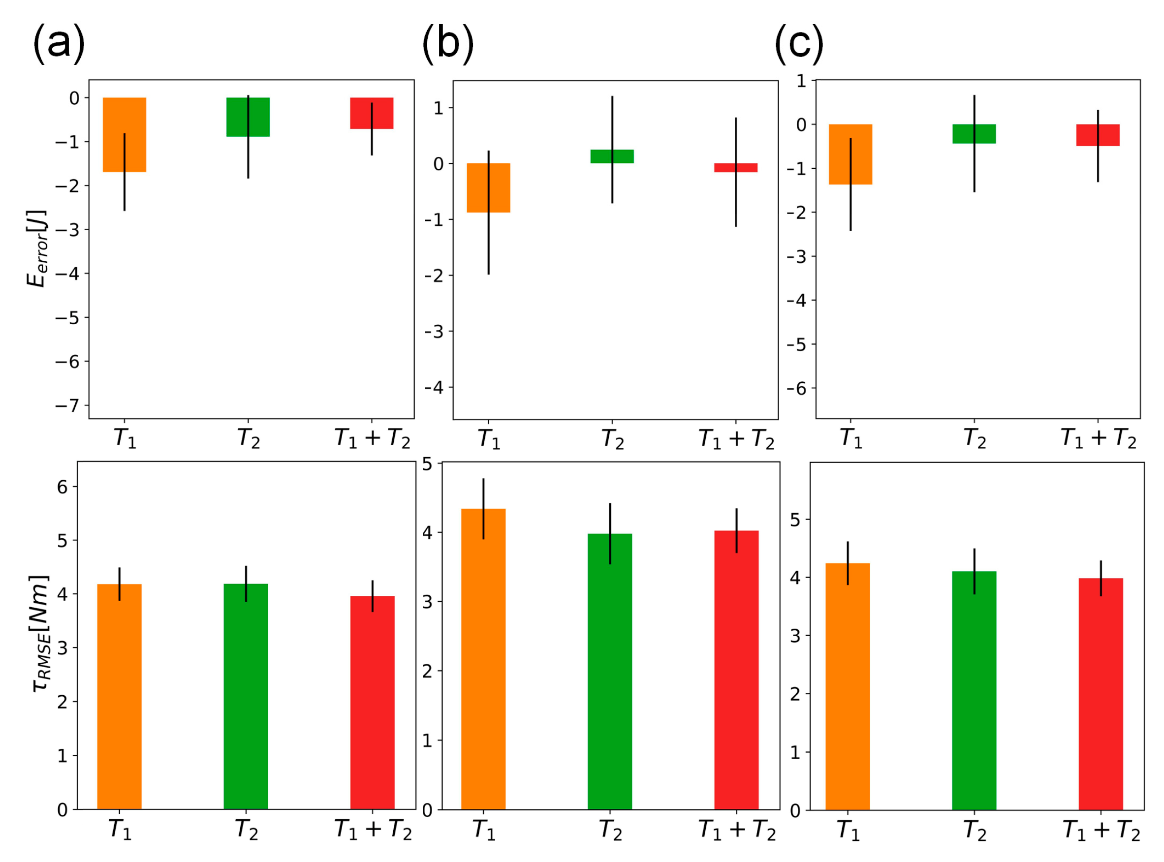
The hybrid model is composed of a reduced-order analytic model, a linear empirical compensation, and a DNN model. To spare computing complexity, the analytic dynamic model was reduced to a three-DOF manipulator, with the other links fixed as a mass point, and constructed given mechanical parameters from specification. The empirical part, compensating for inertia, damping, and friction, and the DNN model, ameliorating for the rest of the un-modeled dynamics, were both trained by actual torque data. The experimental results showed that averaged energy errors between the manipulator results and the analytic model (${\tau }_{analytic}$), the analytic model with energy loss terms (${\tau }_{analytic}+{\tau }_{loss}$), and the hybrid model (${\tau }_{hybrid}={\tau }_{analytic}+{\tau }_{loss}+{\tau }_{DNN}$), are −22.1, −2.1, and −0.2 J, respectively, which confirms that the hybrid composition of the model can significantly augment energy estimation accuracy. In cases where the manipulator was subjected to different payloads, the results exhibited a similar trend in amelioration.

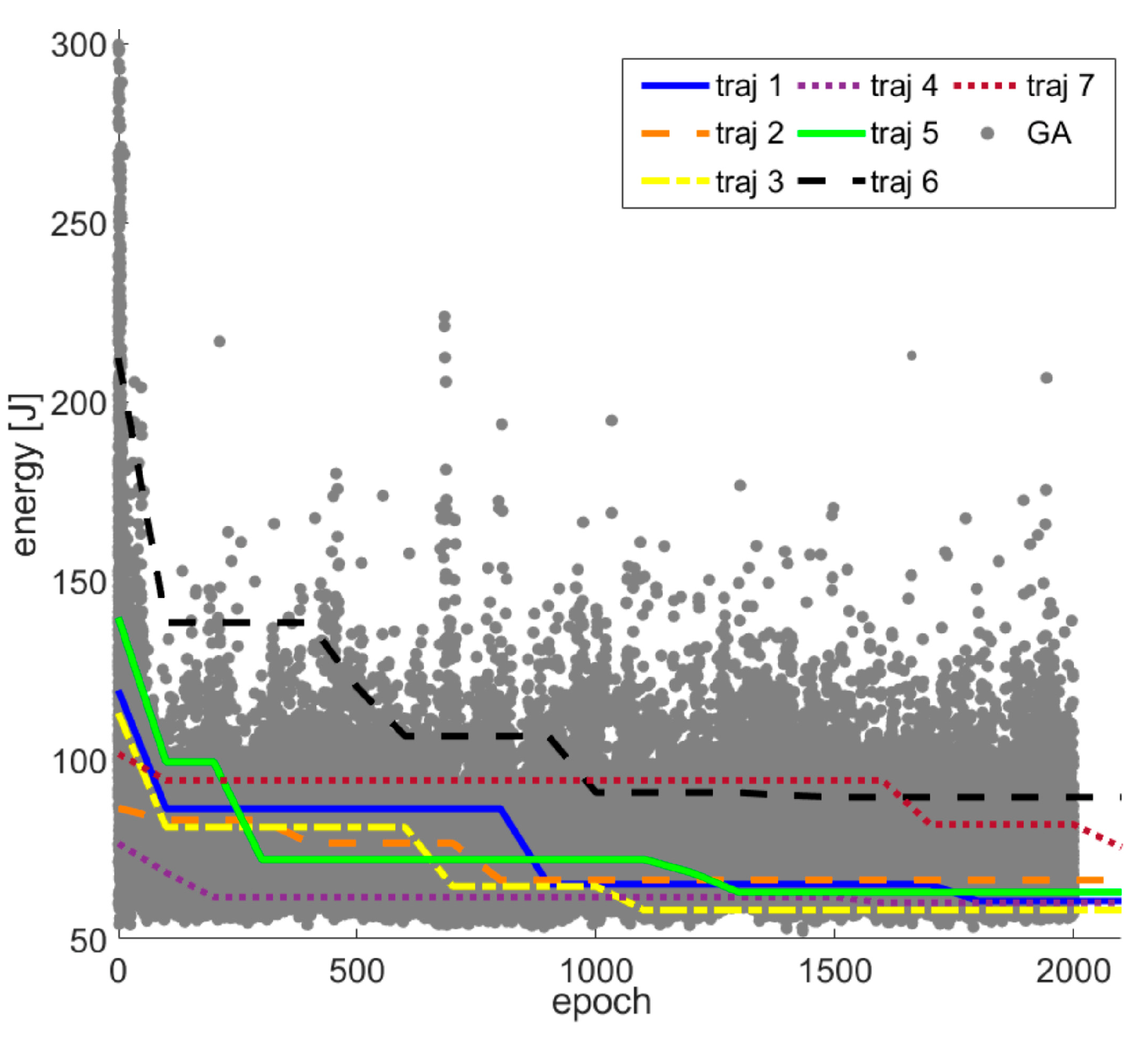
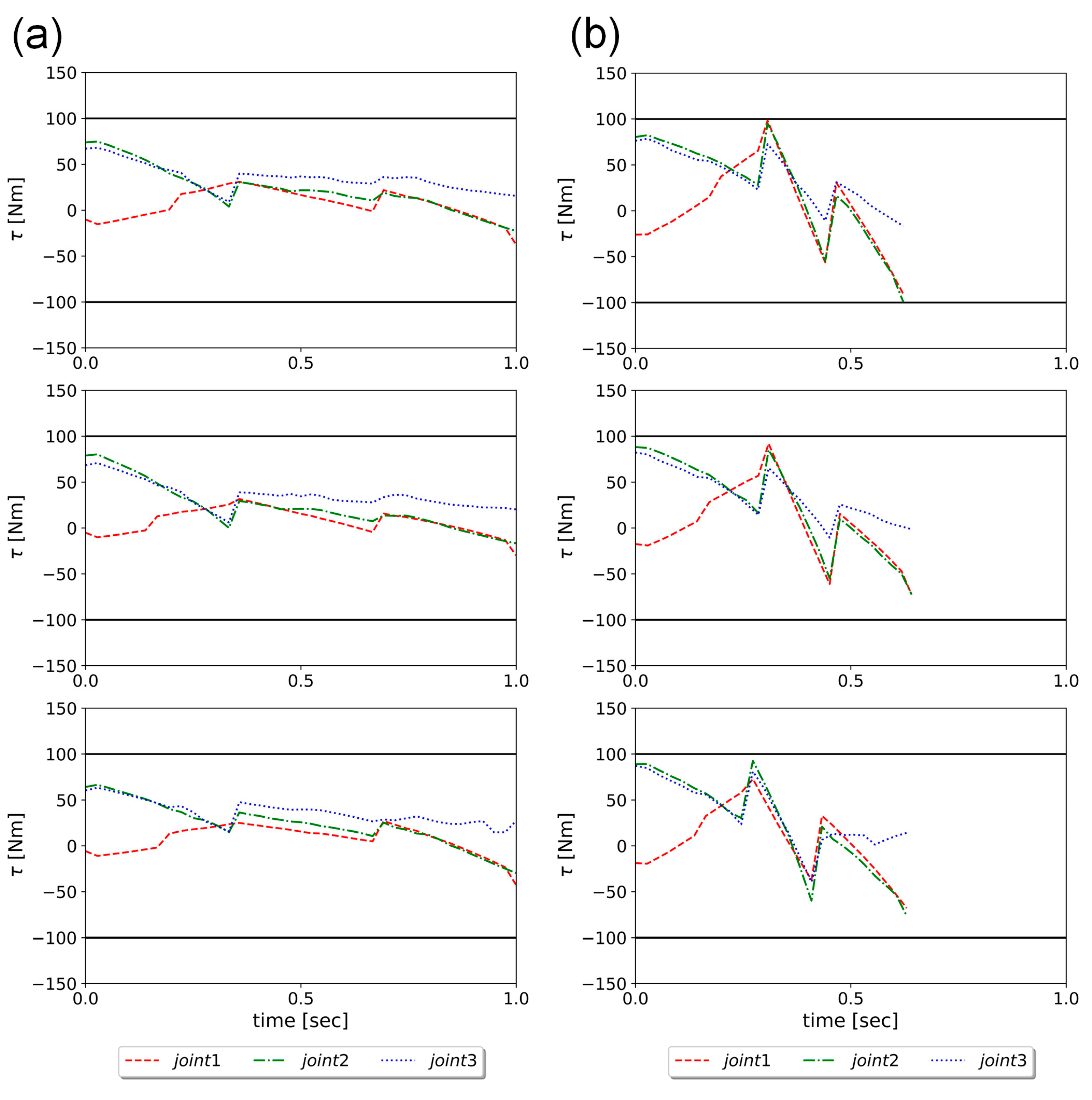
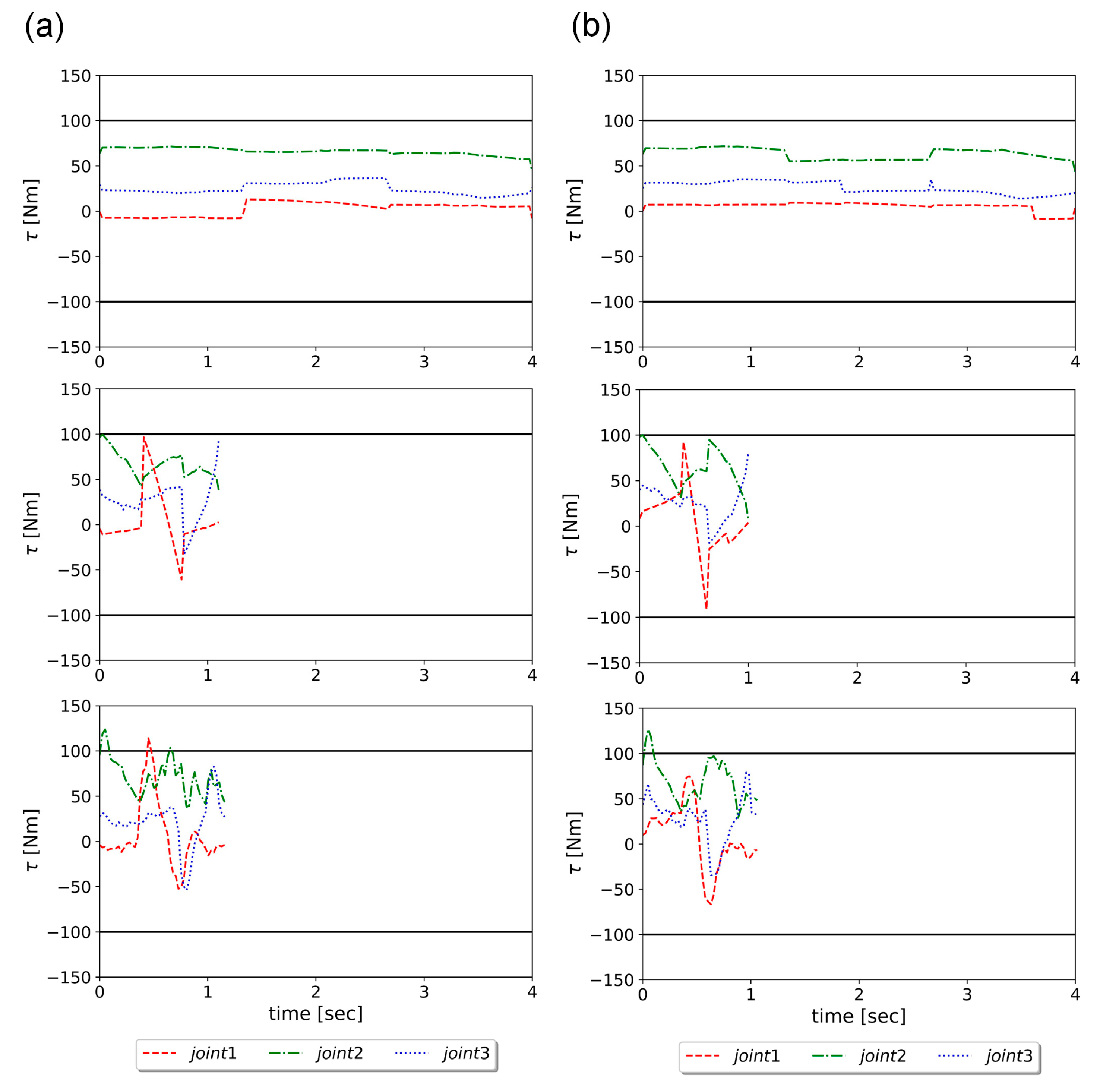
Afterwards, the hybrid model was used in the manipulator trajectory optimization for energy efficiency and speed. The optimization was treated as a bandit problem and solved by RL. The Bi-RRT was utilized to find the initial via points of the trajectories, and then the PPO algorithm was used for trajectory optimization with an obstacle-avoidance capability. In addition, the trajectory optimization using GA was implemented for a performance comparison as well. The simulation results showed that RL can reach almost the same optimization effect as GA, but using only one tenth of the computation time of GA. In the energy optimization experiment, the human-taught method was compared to RL, and the results showed that the energy consumption of the 15 trajectories designed by the testers ranged between 33.9 and 90.9 J, while that of the five trajectories derived by RL had a mean and STD 33.1 ± 0.7 J, attesting to the effectiveness of energy optimization using RL. For the speed optimization experiments, the performance of the RL method was better than that of the time compression method by approximately 27%. In short, RL can effectively reduce energy and time consumption in the manipulator obstacle-avoiding tasks with much less computation time compared to other optimization algorithms.

We are currently working on using different artificial intelligence techniques for the same energy and speed optimization problem as well as deploying the developed technique for other types of manipulators. Moreover, more efficient algorithms are also being investigated. The PPO algorithm can be deployed in the same way as the distributed PPO (DPPO) to augment the solution searching space and speed up optimization convergence. The hyperparameters of the NN structure can be further optimized by using Bayesian optimization.

References

1. Singh, S.; Leu, M.-C. Optimal trajectory generation for robotic manipulators using dynamic programming. J. Dyn. Syst. Meas. Control. 1987, 109, 88–96. [Google Scholar] [CrossRef]
2. Field, G.; Stepanenko, Y. Iterative dynamic programming: An approach to minimum energy trajectory planning for robotic manipulators. In Proceedings of the IEEE International Conference on Robotics and Automation (ICRA), Minneapolis, MN, USA, 22–28 April 1996; pp. 2755–2760. [Google Scholar]
3. Hirakawa, A.R.; Kawamura, A. Trajectory planning of redundant manipulators for minimum energy consumption without matrix inversion. In Proceedings of the IEEE International Conference on Robotics and Automation (ICRA), Albuquerque, NM, USA, 20–25 April 1997; pp. 2415–2420. [Google Scholar]
4. Gregory, J.; Olivares, A.; Staffetti, E. Energy-optimal trajectory planning for robot manipulators with holonomic constraints. Syst. Control. Lett. 2012, 61, 279–291. [Google Scholar] [CrossRef]
5. Hansen, C.; Öltjen, J.; Meike, D.; Ortmaier, T. Enhanced approach for energy-efficient trajectory generation of industrial robots. In Proceedings of the IEEE International Conference on Automation Science and Engineering (CASE), Seoul, Republic of Korea, 20–24 August 2012; pp. 1–7. [Google Scholar]
6. Wigstrom, O.; Lennartson, B.; Vergnano, A.; Breitholtz, C. High-level scheduling of energy optimal trajectories. IEEE Trans. Autom. Sci. Eng. 2013, 10, 57–64. [Google Scholar] [CrossRef] [Green Version]
7. Hollerbach, J.; Suh, K. Redundancy resolution of manipulators through torque optimization. In Proceedings of the IEEE International Conference on Robotics and Automation (ICRA), St. Louis, MO, USA, 25–28 March 1985; pp. 1016–1021. [Google Scholar]
8. Suh, K.; Hollerbach, J. Local versus global torque optimization of redundant manipulators. In Proceedings of the IEEE International Conference on Robotics and Automation (ICRA), Raleigh, NC, USA, 31 March–3 April 1987; pp. 619–624. [Google Scholar]
9. Sahar, G.; Hollerbach, J.M. Planning of minimum-time trajectories for robot arms. Int. J. Robot. Res. 1986, 5, 90–100. [Google Scholar] [CrossRef] [Green Version]
10. Gasparetto, A.; Zanotto, V. Optimal trajectory planning for industrial robots. Adv. Eng. Softw. 2010, 41, 548–556. [Google Scholar] [CrossRef]
11. Rubio, F.; Llopis-Albert, C.; Valero, F. Industrial robot efficient trajectory generation without collision through the evolution of the optimal trajectory. Robot. Auton. Syst. 2016, 86, 106–112. [Google Scholar] [CrossRef] [Green Version]
12. Ghasemi, M.; Kashiri, N.; Dardel, M. Time-optimal trajectory planning of robot manipulators in point-to-point motion using an indirect method. Proc. Inst. Mech. Eng. Part C: J. Mech. Eng. Sci. 2012, 226, 473–484. [Google Scholar] [CrossRef]
13. Schulman, J.; Duan, Y.; Ho, J.; Lee, A.; Awwal, I.; Bradlow, H.; Pan, J.; Patil, S.; Goldberg, K.; Abbeel, P. Motion planning with sequential convex optimization and convex collision checking. Int. J. Robot. Res. 2014, 33, 1251–1270. [Google Scholar] [CrossRef] [Green Version]
14. Krivošej, J.; Šika, Z. Optimization and control of a planar three degrees of freedom manipulator with cable actuation. Machines 2021, 9, 338. [Google Scholar] [CrossRef]
15. Choi, Y.; Jimenez, H.; Mavris, D.N. Two-layer obstacle collision avoidance with machine learning for more energy-efficient unmanned aircraft trajectories. Robot. Auton. Syst. 2017, 98, 158–173. [Google Scholar] [CrossRef]
16. Garg, D.P.; Kumar, M. Optimization techniques applied to multiple manipulators for path planning and torque minimization. Eng. Appl. Artif. Intell. 2002, 15, 241–252. [Google Scholar] [CrossRef] [Green Version]
17. Tian, L.; Collins, C. An effective robot trajectory planning method using a genetic algorithm. Mechatronics 2004, 14, 455–470. [Google Scholar] [CrossRef]
18. Števo, S.; Sekaj, I.; Dekan, M. Optimization of robotic arm trajectory using genetic algorithm. IFAC Proc. Vol. 2014, 47, 1748–1753. [Google Scholar] [CrossRef] [Green Version]
19. Abu-Dakka, F.J.; Assad, I.F.; Alkhdour, R.M.; Abderahim, M. Statistical evaluation of an evolutionary algorithm for minimum time trajectory planning problem for industrial robots. Int. J. Adv. Manuf. Technol. 2017, 89, 389–406. [Google Scholar] [CrossRef]
20. Glasius, R.; Komoda, A.; Gielen, S.C. Neural network dynamics for path planning and obstacle avoidance. Neural Netw. 1995, 8, 125–133. [Google Scholar] [CrossRef]
21. Martín, P.; Millán, J.d.R. Robot arm reaching through neural inversions and reinforcement learning. Robot. Auton. Syst. 2000, 31, 227–246. [Google Scholar] [CrossRef]
22. Imajo, S.; Konishi, M.; Nishi, T.; Imai, J. Application of a neural network to the generation of a robot arm trajectory. Artif. Life Robot. 2005, 9, 107–111. [Google Scholar] [CrossRef]
23. Levine, S.; Pastor, P.; Krizhevsky, A.; Ibarz, J.; Quillen, D. Learning hand-eye coordination for robotic grasping with deep learning and large-scale data collection. Int. J. Robot. Res. 2016. [Google Scholar] [CrossRef]
24. Qiao, L.; Luo, X.; Luo, Q. Control of trajectory tracking for mobile manipulator robot with kinematic limitations and self-collision avoidance. Machines 2022, 10, 1232. [Google Scholar] [CrossRef]
25. Kober, J.; Bagnell, J.A.; Peters, J. Reinforcement learning in robotics: A survey. Int. J. Robot. Res. 2013, 32, 1238–1274. [Google Scholar] [CrossRef] [Green Version]
26. Stulp, F.; Theodorou, E.A.; Schaal, S. Reinforcement learning with sequences of motion primitives for robust manipulation. IEEE Trans. Robot. 2012, 28, 1360–1370. [Google Scholar] [CrossRef]
27. Cheng, Y.; Zhang, W. Concise deep reinforcement learning obstacle avoidance for underactuated unmanned marine vessels. Neurocomputing 2018, 272, 63–73. [Google Scholar] [CrossRef]
28. Cao, Z.; Guo, H.; Zhang, J.; Oliehoek, F.; Fastenrath, U. Maximizing the probability of arriving on time: A practical Q-learning method. In Proceedings of the AAAI Conference on Artificial Intelligence, San Francisco, CA, USA, 4–9 February 2017; pp. 4481–4487. [Google Scholar]
29. Kollar, T.; Roy, N. Trajectory optimization using reinforcement learning for map exploration. Int. J. Robot. Res. 2008, 27, 175–196. [Google Scholar] [CrossRef]
30. Akrour, R.; Abdolmaleki, A.; Abdulsamad, H.; Neumann, G. Model-free trajectory optimization for reinforcement learning. In Proceedings of the International Conference on Machine Learning (ICML), New York, NY, USA; 2016; pp. 2961–2970. [Google Scholar]
31. Li, Z.; Zhao, T.; Chen, F.; Hu, Y.; Su, C.-Y.; Fukuda, T. Reinforcement learning of manipulation and grasping using dynamical movement primitives for a humanoidlike mobile manipulator. IEEE/ASME Trans. Mechatron. 2018, 23, 121–131. [Google Scholar] [CrossRef]
32. Bucinskas, V.; Dzedzickis, A.; Sumanas, M.; Sutinys, E.; Petkevicius, S.; Butkiene, J.; Virzonis, D.; Morkvenaite-Vilkonciene, I. Improving industrial robot positioning accuracy to the microscale using machine learning method. Machines 2022, 10, 940. [Google Scholar] [CrossRef]
33. Hsu, F.-S.; Perng, C.-K.; Ding, H.-M.; Chen, Y.-H.; Yu, H.-J.; Lu, C.-C.; Wu, Y.-J.; Chen, C.-M. Postoperative free-flap registration and tracking system using robotic arm with embedded camera. In Proceedings of the IEEE International Symposium on Biomedical Imaging (ISBI), Washington, DC, USA, 4–7 April 2018. [Google Scholar]
34. Lee, C.-E.; Chen, C.-M.; Hsu, F.-S.; Yu, H.-J.; Chen, L.-W.; Yang, A.-S.; Perng, C.-K. A Postoperative Free Flap Monitoring System: Circulatory Compromise Detection Based on Visible-Light Image. IEEE Access 2022, 10, 4649–4665. [Google Scholar] [CrossRef]
35. Rethink Robotics, Sawyer BLACK Edition. Available online: https://www.rethinkrobotics.com/fileadmin/user_upload/sawyer/rr-blackedition-brochure_low.pdf (accessed on 24 February 2023).
36. Universal Robots, UR5e. Available online: https://www.universal-robots.com/products/ur5-robot/ (accessed on 24 February 2023).
37. Franka Emika, Panda Robots. Available online: https://www.franka.de/research (accessed on 24 February 2023).
38. Gottschalk, S.; Lin, M.C.; Manocha, D. OBBTree: A hierarchical structure for rapid interference detection. In Proceedings of the Proceedings of the 23rd Annual Conference on Computer Graphics and Interactive Techniques, New Orleans, LA, USA, 4–9 August 1996; pp. 171–180.
39. Gottschalk, S. Separating Axis Theorem; Technical Report TR96-024; Department of Computer Science, UNC Chapel Hill: Chapel Hill, NC, USA, 1996. [Google Scholar]
40. Eberly, D. Dynamic Collision Detection Using Oriented Bounding Boxes; Geometric Tools, Inc.: Chapel Hill, NC, USA, 2002. [Google Scholar]
41. Craig, J.J. Introduction to Robotics: Mechanics and Control; Pearson/Prentice Hall Upper: Saddle River, NJ, USA, 2005; Volume 3, pp. 201–229. [Google Scholar]
42. Inc., T.R. TM AI Cobot. Available online: https://tm-robot.oss-cn-hongkong.aliyuncs.com/Single%20Download%20File/SPEC%2022J31EN.pdf (accessed on 7 February 2023).
43. Schulman, J.; Wolski, F.; Dhariwal, P.; Radford, A.; Klimov, O. Proximal policy optimization algorithms. arXiv 2017, arXiv:1707.06347. [Google Scholar]
44. Heess, N.; TB, D.; Sriram, S.; Lemmon, J.; Merel, J.; Wayne, G.; Tassa, Y.; Erez, T.; Wang, Z.; Eslami, S.M.A.; et al. Emergence of locomotion behaviours in rich environments. arXiv 2017, arXiv:1707.06347. [Google Scholar]
45. Kuffner, J.J.; LaValle, S.M. RRT-connect: An efficient approach to single-query path planning. In Proceedings of the IEEE International Conference on Robotics and Automation (ICRA), Chapel Hill, NC, USA, 24–28 April 2000; pp. 995–1001. [Google Scholar]
46. Ratiu, M.; Prichici, M. Industrial robot trajectory optimization- a review. MATEC Web Conf. 2017, 126. [Google Scholar] [CrossRef] [Green Version]
47. Constantinescu, D.; Croft, E.A. Smooth and time-optimal trajectory planning for industrial manipulators along specified paths. J. Robot. Syst. 2000, 17, 233–249. [Google Scholar] [CrossRef]
48. Mitchell, M. An Introduction to Genetic Algorithms; The MIT Press: Cambridge, MA, USA, 1996. [Google Scholar]
49. Lee, J.H.; Park, J.H. Time-dependent genetic algorithm and its application to quadruped’s locomotion. Robot. Auton. Syst. 2019, 112, 60–71. [Google Scholar] [CrossRef]
Figure 1. The manipulator and the model: (a) a photograph of the manipulator for experimental validation, (b) schematic diagram and coordinate systems of the manipulator, and (c) the three-DOF reduced-order model of the manipulator.
Machines 11 00350 g001
Figure 2. The overall construction framework of the hybrid dynamic model.
Machines 11 00350 g002
Figure 3. The flow chart of the self-collision detection.
Machines 11 00350 g003
Figure 4. The manipulator covered by the bounding boxes ready to check collision, where the green box is Link 1, the blue box is Link 2, the red box is Link 3, and the gray boxes are the combination of Links 4 to 6.
Machines 11 00350 g004
Figure 5. The actor-critic structure in the proximal policy optimization (PPO).
Machines 11 00350 g005
Figure 6. The optimization algorithm for via points.
Machines 11 00350 g006
Figure 7. The genetic algorithm (GA) procedure as the compared baseline. More detailed concepts of GA can refer to [48].
Machines 11 00350 g007
Figure 8. The trajectory data groups used for constructing the DNN model of the manipulator. The training trajectories T1 shown in (a) and T2 shown in (b). The evaluation trajectories E1 shown in (c) and E2 shown in (d).
Machines 11 00350 g008
Figure 9. The errors of the manipulator energy consumption and the RMSE of the joint torques. Subfigures (ac) are the results using the evaluating trajectory data groups, E1, E2, and E1 + E2, respectively. In each subfigure, three bars represent the performance of the hybrid model by training data groups T1, T2, and T1 + T2, where black lines are plus and minus one STD and colored bars are mean values.
Machines 11 00350 g009
Figure 10. The total energy consumption of the model versus the computation epoch using the RL algorithm and GA. The proposed RL learning algorithm utilizes seven initial trajectories found by Bi-RRT.
Machines 11 00350 g010
Figure 11. The joint torque profiles of the model (a) before and (b) after speed optimization. The rows represent three different trials. The black solid lines represent the torque limits.
Machines 11 00350 g011
Figure 12. The (a) start and (b) end configurations of the manipulator in the experiment. The red shaded box is the obstacle placed on top of a desk, which is shown as transparent. The solid boxes represent the bounding boxes of the manipulator. (c) A photograph of the experimental setup.
Machines 11 00350 g012
Figure 13. The speed optimization results. From the top: the joint torque profiles of the hybrid model before (1st row) and after (2nd row) speed optimization and of the manipulator (3rd row). The profiles shown in (a,b) were optimized from different energy-optimized trajectories: (a) using Bi-RRT generated via points and (b) using human-taught via points. All plots were drawn using Python and Matplotlib.
Machines 11 00350 g013