Article

LSTM-Based Multi-Task Method for Remaining Useful Life Prediction under Corrupted Sensor Data

College of Intelligence and Computing, Tianjin University, Tianjin 300350, China
*
Author to whom correspondence should be addressed.
Machines 2023, 11(3), 341; https://doi.org/10.3390/machines11030341
Submission received: 2 February 2023 / Revised: 17 February 2023 / Accepted: 21 February 2023 / Published: 1 March 2023
(This article belongs to the Section Machines Testing and Maintenance)

Abstract

:
Data-driven remaining useful life (RUL) prediction plays a vital role in modern industries. However, unpredictable corruption may occur in the collected sensor data due to various disturbances in the real industrial conditions. To achieve better RUL prediction performance under this situation, we propose a novel multi-task method for RUL prediction, which is named multi-task deep long short-term memory (MTD-LSTM). In MTD-LSTM, convolutional neural network (CNN) and long short-term memory (LSTM) are first employed for feature extraction and fusion. Then, the extracted features are fed into the multi-task learning module, which contains missing value imputation and RUL prediction module. The missing values imputation task and RUL prediction task are performed simultaneously. The purpose of the missing value imputation is to obtain integral degradation information by recovering the complete data; thus, the RUL prediction task performs better under corrupted sensor data. In addition, a novel loss term is proposed to smooth the RUL prediction results without any manual post-processing. The effectiveness of the proposed method is verified on the simulated dataset based on the C-MAPSS dataset.

1. Introduction

With the rapid development of technology, the modern industrial system has become more and more integrated and sophisticated. The increasing complexity and uncertainty of the system has led to a higher need for accurate and efficient prognostics and maintenance. To deal with this problem, prognostics and health management (PHM) is proposed. PHM plays a crucial role in modern industry because it aims at reducing maintenance costs, improving reliability, and enhancing performance [1]. A PHM system can effectively detect the early faults of components of machinery, monitor and predict the degradation process, and help in developing or automatically triggering maintenance schedules and management decisions [2]. Remaining useful life (RUL) prediction is a vital approach for prognostics and a crucial part of the PHM system. The RUL of a system is defined as “ the time from the current time to the end of the useful life” [3]. Accurate RUL prediction result is the basis for efficient and reliable health management and maintenance. For example, for aero engines, if its RUL can be predicted accurately, we can develop a maintenance schedule in advance and replace components with potential failure risks. Thus, the operating life is extended and maintenance costs are reduced. Additionally, possible casualties are avoided.
RUL prediction approaches can be roughly divided into model-based approaches, data-driven approaches, and hybrid approaches. Model-based approaches describe the degradation processes of machinery through building mathematical models on the basis of the failure mechanisms or the first principle of damage [4]. For example, a Paris–Erdogan (PE) model-based RUL prediction method under the framework of Bayesian estimation is proposed in [5], and the system state transition is described with the PE model. However, model-based approaches require a large amount of prior expertise, which is often hard to obtain, and it is increasingly difficult to build accurate physical models due to the increasing complexity of industrial systems. With the gradual improvement of signal processing and feature extraction technology, condition monitoring (CM) using dedicated sensors can provide a large amount of real-time health information for the system. These informative data provide the possibility to construct more effective RUL prediction methods. Data-driven approaches try to utilize machine learning techniques to learn the degradation patterns from monitoring data, so the RUL of systems can be accurately predicted.
A large number of data-driven approaches have been proposed, such as a support vector regression (SVR)-based method [6,7], a hidden Markov model (HMM)-based method [8,9], an artificial neural network (ANN)-based method [10], etc. reference [6], an SVR-based method was proposed for RUL prediction of lithium-ion batteries (LIBs), where the artificial bee colony (ABC) algorithm was utilized for optimization of kernel parameters. HMM-based methods are another important class of RUL prediction methods. For example, Liu et al. [8] proposed a novel switching hidden semi-Markov model (SHSMM) to represent the degradation process of equipment, and it has a more generalized form and a more powerful ability to describe the degradation process with time-varying working mode compared to traditional HMM-based methods. The ANN-based methods have actually developed into the most popular methods currently in use, i.e., the deep learning method. Deep learning is a popular branch of machine learning technology. It can extract deep features and degradation information from original monitoring data without any manual operation, so it can effectively model the degradation process of the monitored system. Therefore, the RUL prediction methods based on deep learning have also been widely studied. In reference [11], a method using a multi-scale deep convolutional neural network (CNN) with an attention mechanism is proposed to effectively fuse multi-sensor data and learn representations from different temporal scales.
Recurrent neural network (RNN) is a classic method that can model the temporal correlation, and long short-term memory (LSTM) [12] is an upgraded version of RNN. Its purpose is to overcome the gradient vanishing and exploding problem. Due to its outstanding performance on temporal sequences modeling, it has been widely used in speech recognition [13], natural language processing [14], and other fields. In industrial big data analysis, the benefit is from its suitability for processing time-series vibration signals that widely exist and are collected in industrial systems. RUL prediction methods based on RNNs and LSTMs have also been widely studied [15,16,17,18,19,20,21,22]. Ren et al. [16] proposed a novel architecture that combined deep CNN and LSTM, which is called Auto-CNN-LSTM. The method overcame the problem of insufficient data in RUL prediction due to the ability of mining deeper information from finite data. In [22] researchers proposed a convolution-based long short-term memory (CLSTM) network by cleverly embedding CNN into LSTM, which not only preserves the advantages of LSTM but also incorporates time-frequency features. These data-driven methods can avoid the problem of building physical models, which is usually hard in real applications. Since acquiring a large amount of monitoring data and powerful computing resources required by the data-driven method has become a reality, and due to the characteristic of model-free and expertise-free, data-driven methods had attracted increased attention and have became the most promising direction in RUL prediction.
In practice, there is a large number of disturbances in industrial sites such as vibrations, shock, electromagnetic interference, chemical corrosion, etc., which lead to unpredictable corrupted sensor data. Ordinary data-driven methods will fail with corruption in the input data because these models are often trained from complete data; therefore, what these models modeled is the distribution of the complete data. However, the corruption in the input data in real applications is not present in the training data, which means it deviates from the distribution of the training data, and the model cannot generalize well. Therefore, it is necessary to introduce corruption data in the training process. A naive way is to directly train the model with the corrupted data, but the learning ability of the model will be challenged, since the unpredictability of the corruption values leads it to be close to random noises, which is hard for machine learning to deal with. Another method is to complement the corrupted values and perform the RUL prediction with the complementary data, including a mean value imputation, matrix completion, deep learning-based methods, etc. However, these operations will introduce imputation errors and human interference, resulting in limited RUL prediction performance.
To cope with the problem mentioned above, a novel RUL prediction method which can perform well under corrupted sensor data is proposed in this work. The architecture of the proposed model is a multi-task framework combining deep LSTM, a missing values imputation task, and an RUL prediction task—the latter two are deployed in parallel following the deep LSTM. With the recovery of missing values, the deep LSTM can fuse the features containing integral degradation information. The hidden representation which greatly benefits RUL prediction in the missing values imputation module is simultaneously used for RUL prediction. Additionally, to further improve the performance of the proposed method, a novel loss term is designed to smooth the predicted RUL. The proposed method is evaluated on the C-MAPSS dataset [23], which is a classical dataset created by NASA and extensively utilized in many RUL prediction studies [21,24,25,26,27]. The high-quality full life degradation data of multiple engines in C-MAPSS greatly helps for comprehensively and objectively evaluating the performance of the proposed method. The main contributions of this work are as follows:
1.
A novel multi-task method is proposed for RUL prediction under corrupted sensor data. With the assistance of the missing values imputation module, the proposed method can perform well in RUL prediction under corrupted sensor data.
2.
A novel loss term is introduced for improving the RUL prediction performance, which can smooth the predicted RUL without any manual post-processing.
3.
Extensive comparative experiments and ablation studies verified the effectiveness of the proposed method.
The rest of this article is organized as follows: Section 2 describes the details of the proposed method, the effectiveness of the proposed method is verified in Section 3, and, finally, Section 4 concludes this work.

2. Methodology

2.1. Problem Statement

In industrial systems, the collected data from the sensor network is usually time-series signals, such as vibration signals, acoustic signals, temperature, voltage, etc. In the RUL prediction task, vibration signals are the most commonly used. The proposed method utilizes a deep model to extract degradation information from the vibration signals for RUL prediction. The common multi-sensor RUL prediction task based on the vibration signals can be expressed as: construct a regression model f ( · ) , given multi-sensor time-series signals
X T = [ x T ( 1 ) , x T ( 2 ) , , x T ( s ) ] R T × s
collected until time T, where s denote the number of sensors. Then the RUL at time T can be predicted with
R U L T = f ( X T ) .
However, in real industrial applications, many disturbances can lead to unpredictable corruption in the collected sensor data. It can be assumed that the corrupted data is detected, and thus the value is set equal to zero, which represents a missing value. Thus, the collected signal X ^ T with missing values is:
X ^ T = 0 0 0 x 2 ( 1 ) x 2 ( 2 ) 0 x T ( 1 ) 0 x T ( s ) R T × s .
Therefore, the existing methods based on complete data will fail when encountering missing values. To deal with this problem, a novel RUL prediction method that can process the above-mentioned data with severe random missing values is proposed in this work.

2.2. Overview

The process of the proposed method is as follows: First, the corrupted data is simulated manually based on the complete data; this is a critical part of the proposed method. This is because the mapping from corrupted data to complete data needs to be modeled, which is the missing values imputation task mentioned later, so both complete data and corresponding corrupted data are necessary. The specific simulation process is described in 
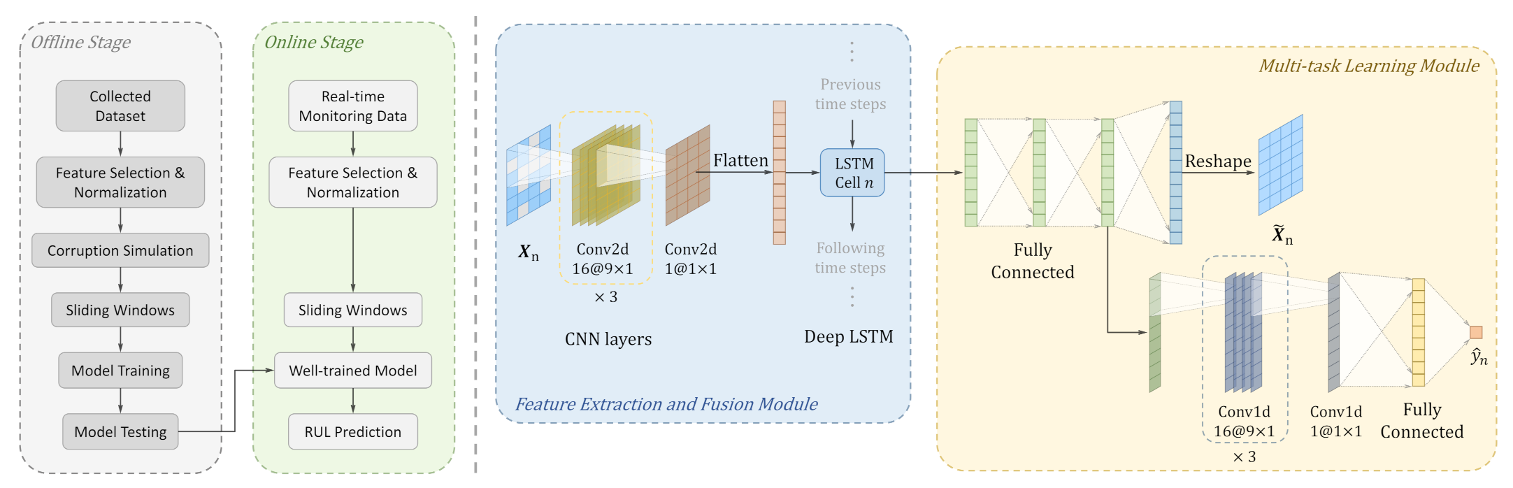
Section 3.3 considering it is a part of data processing. Second, the proposed multi-task deep LSTM (MTD-LSTM) will be trained using the simulated corrupted data and tested using testing samples with corrupted values under different missing rates. Note that the corresponding complete values are not required in the testing process, which is consistent with real applications. Third, the well-trained model will be deployed in real industrial applications. It should be noted that the basic assumption is that the corrupted values of the input data have been detected and replaced by 0 values, and the detection method is not considered in this work. The flowchart of the proposed method is shown in the left part of Figure 1.
The core of the proposed MTD-LSTM is a multi-task learning framework with a deep LSTM. The architecture of MTD-LSTM is shown in the right part of Figure 1. There are two main parts in MTD-LSTM, first, a degradation feature extraction and fusion module consisting of a CNN and a deep LSTM and second, a multi-task learning module consisting of missing value imputation module and RUL prediction module.
Firstly, the signals with missing values are fed into the degradation feature extraction and fusion module to extract and fuse the degradation information, where the CNN and deep LSTM are employed sequentially. CNN is commonly used for feature extraction and the deep LSTM can effectively fuse the extracted features along with time steps. The fused features are next fed into the multi-task learning module for missing value imputation and RUL prediction.
For the RUL prediction task, it is difficult to achieve an accurate prediction if there are missing values in the input data. The reason lies in that the missing values lead to the loss of degradation information. To deal with this, multi-task learning is utilized. Specifically, the missing values imputation module is implemented to recover the complete data. That being the case, the hidden representation in the missing values imputation module contains the integral degradation information. Based on the idea of multi-task learning, the hidden representation containing integral degradation information is used for RUL prediction simultaneously, thus a better RUL prediction performance can be achieved. Moreover, the proposed monotone and linearly decreasing loss (MoLD Loss) is imposed on the predicted RUL for smoother results.

2.3. Feature Extraction and Fusion Module

In the feature extraction and fusion module, the CNN and deep LSTM are utilized to extract and fuse the features from the input data with missing values. CNN was originally used in computer vision; however, some studies show it also performs well in processing time-series signals [28]. Here, we utilized CNN for local feature extraction on the input data with missing values. The original multi-sensor signals are firstly processed into samples by the sliding window technique. The input sample n can be expressed as X n = [ x n ( 1 ) , x n ( 2 ) , , x n ( s ) ] R w × s where w and s denote window size and the number of sensors. We implemented a 4-layer CNN model with tanh activation function to extract local features from the input samples. The details of the CNN model are shown in Figure 1. Note that the output feature map is reshaped into a vector to adapt the input dimension of deep LSTM. Only using the CNN model to extract the local feature is not enough for RUL prediction under corrupted sensor data because the severe missing values may occur in sample X n , which will lead to severe degradation information loss. Therefore, the historical information in the previous samples must be considered and temporal correlations must be modeled to fully explore the available information under corrupted sensor data.
Here, the deep LSTM is employed following CNN to model the temporal correlations, and features extracted from past time steps are fused. An LSTM consists of a series of units; the structure of the unit is shown in Figure 2. The input at time t includes current data x t R d × 1 , the hidden state h t 1 R m × 1 , and the memory cell state c t 1 R m × 1 from time t 1 . After calculation, c t and h t passed the long-term memory and short-term memory along with new information from x t on to next unit. This mechanism is achieved by controlling the data flow through control gates, namely, the input gate, forget gate, and output gate, which are shown in Figure 2. In deep LSTM, the hidden state of the previous layer is used as the input data for the next layer.
In LSTM, since the memory cell state and hidden state contain long-term and short-term memory, respectively, they contain abundant historical degradation information in different stages. This provides the possibility of recovering the complete data X ^ n in the following missing values imputation task, even if X n is highly incomplete. By iteratively inputting the samples before sample n into the model, the deep LSTM can model the temporal correlations of the time series signals, and the output hidden representation h n of sample n integrated the historical degradation information. Moreover, the deep LSTM can fully explore the correlation between different sensors to make full use of the available information in X n for recovering the missing values. So, the extracted h n fully integrated the available information and leads to effective missing values imputation followed by a better RUL prediction performance, even if the input data X n is highly incomplete.

2.4. Multi-Task Learning

After extracting and fusing the degradation features from the input data with missing values, the hidden representation h n will be fed into the multi-task learning module for missing value imputation and RUL prediction tasks.
In the missing values imputation module, h n output by the deep LSTM at time step n is used for recovering the complete data X ^ n corresponding to the incomplete input X n . To map h n from hidden representation space to high-dimensional observation space, a 3-layer fully connected network (FCN) is implemented in this module. The output vector of this module is reshaped to a matrix X ˜ n R w × s to adapt the samples’ dimension. Due to the strong fitting ability of FCN, it can fit the detailed information in the complete data X ^ n to recover the missing values from h n . In this module, the rectified linear unit (ReLU) activation function is used for nonlinear transformation. The target of the missing values imputation task is to let the output of the module be as similar as possible to the complete data. Mean squared error (MSE) is used as the loss function to measure the error between the output and the complete data. Assuming that X ˜ n and X ^ n denote the output and the complete data of sample n, the imputation loss is
L i m p = 1 w s N n = 1 N | | X ^ n X ˜ n | | F 2 ,
where N, w, and s denote the number of total samples, window size, and the number of sensors, respectively.
Missing values imputation is not the final goal, but an auxiliary means for RUL prediction under corrupted sensor data. For prediction, an RUL prediction module is employed that shares the first two layers of FCN with the missing values imputation module. Following the shared layers, a 4-layer 1D CNN is utilized to extract the degradation features from the hidden representation. Note that the hidden representation is shared for the missing values imputation task, which means the shared representation contains the integral degradation information, and this greatly benefits RUL prediction. The details of the 1D CNN model are shown in Figure 1. Following the 1D CNN, a 2-layer FCN with 512 neurons in the hidden layer is employed to fit the target RUL from the extracted features. The commonly used MSE loss in regression tasks is utilized to calculate the prediction error. Assuming that y ^ n and y n denote the predicted value and the target RUL of sample n, the prediction loss is
L p r e d = 1 N t = 1 N ( y ^ n y n ) 2 ,
where N denotes the number of total samples. In order to let the missing values imputation task assist RUL prediction, the overall loss function is
L = L p r e d + α · L i m p ,
where α denotes the weight of L i m p .

2.5. Monotone and Linearly Decreasing Loss

For the purpose of improving the smoothness of RUL prediction, a monotone and linearly decreasing (MoLD) loss term is applied to the prediction results. This term is inspired by the nature of RUL: monotone and linear decline. Specifically, we assume that y ^ n and y ^ n Δ denote the predicted RUL of sample n and the sample Δ time steps earlier than n, respectively, and Δ y ^ n = y ^ n Δ y ^ n denotes the difference between y ^ n Δ and y ^ n . Ideally, Δ y ^ n should be equal to Δ according to the nature of RUL mentioned above. However, in practice, due to the effect of the limited performance of the model, the noise in the collected signal, and the missing value in the data, Δ y ^ n is usually not equal to Δ , which means the fluctuation of prediction results. A common approach is to apply smoothing post-processing to the prediction results, but it is cumbersome and human interference is introduced to the output of the model. To let the model output the smoothed RUL directly, we propose to add the MoLD loss term L M o L D to Equation (6) to constrain the RUL prediction result, which leads the model to directly output a smooth RUL prediction:
L = L p r e d + α · L i m p + β · L M o L D ,
where β denotes the weight of L M o L D and
L M o L D = 1 T Δ t = 1 + Δ T | y ^ t Δ y ^ t Δ | ,
where Δ is a hyper-parameter to control the intensity of smoothness. Intuitively, if y ^ n Δ y ^ n = Δ , there is no penalty on the result. However, whether the predicted value is greater or less than the ideal value, a penalty will be imposed on the result. In other words, the RUL prediction result will be locally smoothed without any manual post-processing.

3. Experimental Study

3.1. Dataset Description

In this study, a simulated turbofan engine degradation dataset [23] is used to evaluate the effectiveness of the proposed method. This dataset is created by NASA and is called C-MAPSS. They developed a model-based aircraft engine degradation simulation program to simulate the engine degradation process in different fault modes and operating conditions, then multi-sensor degradation signals are collected from it. There are four subsets named FD001, FD002, FD003, and FD004 in C-MAPSS, and a training set and testing set are provided in each subset. In each training set, there are multiple run-to-failure degradation trajectories of engines with different degrees of initial damage and have been running to complete failure. However, in each testing set, the collected signals stop at a time point before the engine totally failed. The details of the C-MAPSS dataset are provided in reference [23]. The collected degradation data are multi-sensor signals with 21 sensors, which reflect the degradation process from different views. In this work, since the collected signals from sensor T2, P2, P15, epr, farB, Nf-dmd, and PCNfR-dmd are approximately constants, the degradation information cannot be provided. The performance of the model may not be improved and even be harmed by the useless features if we keep them in the training set. Thus, the useless features are removed and only 14 sensors are retained, which is also a common operation in previous studies [24,25]. The real RUL is provided in all training and testing samples, and we applied piece-wise RUL as the target RUL according to [29]. The details of C-MAPSS dataset are shown in Table 1.

3.2. Evaluation Metrics

To evaluate the performance of the proposed approach, three metrics are utilized in this study. Firstly, the accuracy of RUL prediction is evaluated using root mean square error (RMSE) and the score function [23]. RMSE is widely used in RUL prediction since it is a common evaluation metric in regression tasks. RMSE is calculated with:
R M S E = 1 N n = 1 N ( y ^ n y n ) 2 ,
where N denotes the number of samples; y ^ n and y n stand for the predicted value and the target RUL of sample n, respectively. To some extent it can be seen as the mean error of the prediction and the target.
RMSE imposes the same penalty on early and late prediction. However, earlier and later prediction of RUL will lead to different harms in real applications, namely later prediction may cause more severe accidents since it cannot predict the failure of equipment in time. To deal with this, the scoring function is proposed in reference [23] and widely used in RUL prediction and is also employed in this study. The scoring function is defined as
S C O R E = e = 1 E ( e y ^ e y e 13 1 ) ,   when y ^ e < y e e = 1 E ( e y ^ e y e 10 1 ) ,   when y ^ e y e ,
where E denotes the total number of testing engines; y ^ e and y e denote the predicted RUL and the target RUL of the last sample of engine e, respectively. The scoring function penalizes more severe on late prediction. RMSE and the scoring function are visualized in Figure 3.
Moreover, to quantitatively evaluate the improvement of the smoothness of the predicted RUL by the proposed MoLD loss, we introduce a fluctuation index (FI) which was originally used to assess the degree of fluctuation of time series data. In this work, we utilize the FI to quantitatively evaluate the smoothness of the predicted RUL. The FI is defined as follows:
F I = 1 N 1 n = 2 N | y ^ n y ^ n 1 | ,
where N denotes the number of total predicted RULs. FI evaluates the stability of the predicted RUL by calculating the difference between two RULs at adjacent time steps. A larger FI means less smoothness of the prediction.

3.3. Data Preprocessing

3.3.1. Normalization

As mentioned in Section 3.1, we use the data in C-MAPSS collected from selected 14 sensors where the scale of the collected data from different sensors varies widely. The model will pay too much attention to features on a larger scale and ignore the smaller ones if using these data directly, which also leads to training difficulties and prediction failures. To balance the influence of features with different scales, we use max-min normalization to scale the data into [ 0 , 1 ] :
x norm ( i , j ) = x ( i , j ) x min ( i ) x max ( i ) x min ( i ) i , j ,
where i and j denotes the number of sensors and data points, x ( i , j ) and x norm ( i , j ) stand for raw data and normalized data, and x max ( i ) and x min ( i ) are the maximum and minimum values of sensor i, respectively. What should be noted is that the data in the testing set should be normalized using the maximum and minimum values of the corresponding engine in the training set, since the collected data in the testing set does not last until the end of the engine life. This will keep the distribution of testing data the same with training data.

3.3.2. Corrupted Sensor Data Simulation

In this study, we aim at accurate RUL prediction under corrupted sensor data. In the proposed method, the training procedure requires both incomplete data with missing values and its corresponding complete data, which do not exist in common datasets. Therefore, we need to manually mask some values in the complete data to simulate the required corrupted data.
We masked some values in the training and testing sets in the C-MAPSS dataset according to a preset missing rate p. According to a previous study [30], the importance of different sensors for RUL prediction is different. The corruption of key sensor data will cause serious loss of degradation information, which leads to a failed RUL prediction. Therefore, to improve the robustness of the model under severely corrupted sensor data, we set larger missing rates for key sensors, while ensuring the total missing rate is equal to p. The data of each sensor is randomly masked according to the constructed missing rate, and the masked values are set to 0. Both training and testing sets are processed in the same pattern.
To show the statistical characteristics, we conducted statistics on the dataset under multiple miss rates, including mean value and standard deviation, and showed them in Table 2.

3.3.3. Sliding Window Processing and Label Construction

Sliding window processing is a widely used technique in time-series data processing and RUL prediction [24,25,31]. In this work, the sliding window processing is applied to the time-series signal for data preparation. On the one hand, it helps in extracting the local degradation features in the data. On the other hand, it also plays the role of data augmentation.
Assuming that the length of original time series signal is T, the feature dimension, that is, the number of sensors is s, and a time window with length w slides on the series signal with step size k, then the original signal is processed as a sample sequence { X n } n = 1 T w k + 1 , where X n R w × s . In our experiments, the sliding window length and step size were the same as these in reference [25]. The RUL of sample X n is T w ( n 1 ) × k . As mentioned in Section 3.1, we use the piece-wise RUL in reference [29] as the label, so the final RUL label is:
R U L = min ( R U L e a r l y , T w ( n 1 ) × k ) ,
where R U L e a r l y = 125 in this study.

3.4. Experimental Settings and Results

3.4.1. Experimental Settings

To verify the effectiveness of the proposed method for RUL prediction under corrupted sensor data, we have performed extensive comparative experimental studies on the simulated datasets.
The selected comparison methods include widely used and validated benchmark methods in RUL prediction, including SVR, MLP, DLSTM [15], and two recent state-of-the-art methods in common RUL prediction tasks: namely DCNN [28] and AGCNN [25]. For a better understanding of DCNN and AGCNN, some relevant studies are given in reference [32,33,34]. Note that since the problem of RUL prediction under corrupted sensor data is a relatively novel and frontier problem in the field of industrial big data, no researchers have proposed a widely recognized and accepted method for this problem. Therefore, the comparison methods selected in our experimental studies are all classical methods for RUL prediction.
There are several hyperparameters to be selected in the proposed method. We performed numerous experiments and used the grid searching method to select the proper value. Specifically, the number of layers of the deep LSTM is two, and the hidden size in the LSTM unit is 512. In the objective function, there are three key hyper-parameters α , β , and Δ , which are set to be 0.35 , 2.0 × 10 3 , and 2, respectively; α and β denote the weight of L i m p and L M o L D , respectively; and Δ is a hyper-parameter controlling the intensity of smoothness. Actually, the prediction accuracy is not very sensitive to the value of α and β ; the values given here are recommended values and not strictly optimal. When the values of α and β are in [ 0.25 , 0.55 ] and [ 1.0 × 10 3 , 4.0 × 10 3 ] , respectively, there is no significant difference between the results with the recommended values. For the parameter Δ , it is more critical to select the appropriate value. An excessively large value of Δ can lead to meaningless prediction. During the training process, the Adam optimizer is applied with a learning rate of 0.001 and batch size of 128, and the training is performed for 300 epochs. The weights of the model are initialized with the Xavier uniform initializer [35]. In the selected comparison methods, the SVR and MLP are called from the classic machine learning library s k l e a r n , and the training parameters take the default values. For the DLSTM, we built the model according to the paper and adjusted the parameters to adapt our data dimension. For the AGCNN and DCNN, we built models based on the parameters given in the paper and tuned them until we reproduce the reported results, then applied them to our simulated datasets. All experiments are conducted on a server with 64-bit Ubuntu 18.04, which has a GeForce RTX 2080 Ti GPU with 12 GB memory.

3.4.2. Effectiveness of the Proposed Method

The RUL prediction experiments are performed on FD001 and FD003 with a missing rate of 0∼0.8 to verify the effectiveness of the proposed method. We firstly train the model on the training set of different missing rates and test it on the corresponding testing set. The training time and testing time are listed in Table 3.
Good performance of the imputation task is the premise of high performance of RUL prediction under corrupted data. The imputation results of the test engine 76 in FD001 under 0.3 missing rate were selected for visualization and are shown in Figure 4. Since there is an overlap in the imputation results between adjacent data points, we average the imputation value of the same data point. It shows that the model can effectively impute the corrupted values. We selected some prediction typical prediction results of testing samples and visualized them in Figure 5. The horizontal and vertical axis represents the time and the RUL, respectively. The red dashed line in each subfigure represents the piece-wise RUL label, and the rest of the lines represent the RUL predicted value under different missing rates, as shown in the legend.
It can be seen from the figure that the proposed method achieved remarkable RUL prediction performance under various missing rates, especially when the missing rate is low. The prediction results almost coincide with those when the missing rate is 0. This is because the proposed method has the ability to sufficiently extract and fuse the degradation features from data with only a few missing values. As the missing rate increases, the predicted RUL gradually deviates from the target value, which is inevitable. Although the large missing rate leads to the deviation of the predicted values, it is still relatively efficient to predict the RUL of the system under the data with a large amount of information missing due to data corruption. This is because the proposed method sufficiently extracts the information from the available data, and the degradation features are recovered with the auxiliary of missing values imputation task; therefore, the RUL can be effectively predicted.

3.4.3. Ablation Study

Furthermore, to verify the role of missing values imputation module and MoLD loss in the proposed method, we conducted ablation studies. Specifically, three versions of MTD-LSTM are used for experiments: only using RUL prediction loss, namely MTD-LSTM ; using RUL prediction loss and imputation loss, namely MTD-LSTM *; and the standard version with all three terms in the objective function, namely MTD-LSTM. The experimental results are shown in Figure 6 and Table 4.
Firstly, we conducted comparison experiments using MTD-LSTM and MTD-LSTM * under different missing rates on the FD001 and FD003 subsets to verify the effectiveness of multi-task learning in the RUL prediction under corrupted sensor data. The result is shown in Figure 7. In each subfigure, the horizontal and vertical axis represents different values of missing rates and the RMSE value of prediction, respectively. The blue and red lines denote the prediction results of MTD-LSTM * and MTD-LSTM , respectively. It shows that the performance of MTD-LSTM which only uses RUL prediction loss is close to that of the common deep learning method under corrupted data. This is because MTD-LSTM cannot sufficiently extract and fuse the degradation information under lots of missing values. However, after adding the imputation loss to the objective function, which means multi-task learning, MTD-LSTM * shows significant improvement compared with MTD-LSTM under corrupted data. The reason lies in that the missing value imputation module effectively extracts integral degradation information from the incomplete data by recovering the missing values; therefore, the RUL prediction module performs its role better with the auxiliary of multi-task learning.
Furthermore, the improvement (IMP) is also calculated and shown in the figure. It shows that the improvement of the multi-task learning method is not quite significant when the missing rate is too high or too low; the reason is as follows. For the previous case, although the multi-task method can deal with a certain degree of missing values, it cannot perform well when encountering too many missing values. This is because most of degradation information has been lost, and accurate RUL prediction is not possible. For the latter case, the common deep learning method is sufficient when the loss of degradation information is not serious, and the multi-task method cannot fully exert its advantages. In the range of missing rates from 0.1 to 0.5, the multi-task learning method shows its powerful advantages, which can greatly improve the RUL prediction performance under corrupted sensor data.
Next, we use the standard version MTD-LSTM for verifying the effectiveness of the MoLD loss term. The purpose of this term is to directly improve the smoothness of the predicted RUL. To verify this, we calculated the FI of the predicted RUL output by MTD-LSTM * and MTD-LSTM. The results on FD003 under different missing rates are shown in Table 4. The improvements are also calculated and shown in the table. It shows that the FI of the standard version is significantly lower than the version without the MoLD loss term, which means the MoLD loss term can effectively smooth the predicted RUL. We select some representative RUL prediction results for visualization in Figure 6. The red dashed line represents the RUL label, and the blue and orange lines represent the RUL prediction results of MTD-LSTM * and MTD-LSTM, respectively. Obviously, the prediction results of MTD-LSTM are smoother. This is because the short-term fluctuation is strongly suppressed by the constraint on the two adjacent output values by the MoLD loss term. Therefore, clearer equipment health conditions can be obtained, and more effective equipment maintenance and management decisions can be made.

3.4.4. Comparisons with Other Methods

To further evaluate the superiority of the proposed method, we compared several classical methods with two versions of the proposed method, namely the standard MTD-LSTM and MTD-LSTM * without MoLD loss term. The comparison methods include SVR, MLP, LSTM, DCNN, AGCNN, etc. We use these methods to conduct experiments on FD001 and FD003 subsets under different missing rates. The experimental results evaluated by RMSE and SCORE are shown in Table 5 and Table 6, respectively.
It shows that the proposed method obtains outstanding performance compared with other methods. MTD-LSTM comprehensively outperforms the compared prediction methods under different missing rates, both in RMSE and SCORE. This means that MTD-LSTM can effectively predict the RUL under different degrees of missing values, which traditional RUL prediction methods cannot do. For traditional methods, when encountering a large number of missing values, they cannot extract degradation information from these incomplete data. This is because these methods do not have effective information fusion and extraction mechanisms designed for incomplete input data. For the proposed MTD-LSTM—based on the idea of multi-task learning—the RUL prediction task is performed with auxiliary by missing value imputation task; therefore, the degradation information can be effectively extracted from the incomplete data, which is not achieved by traditional methods. Moreover, the combination of multi-layer LSTM and CNN greatly helps in fully exploring the spatiotemporal correlations in the data, which provides a guarantee for the effectiveness of the missing values imputation task, and then the RUL prediction task is performed more efficiently.

4. Conclusions

In this work, we proposed an LSTM-based multi-task model (i.e., MTD-LSTM) for RUL prediction under corrupted sensor data. The corrupted data is first fed into the feature extraction and fusion module, and the extracted features are next simultaneously sent to the missing values imputation and RUL prediction module. The purpose of the missing values imputation task is to extract integral degradation information from the incomplete data; therefore, the RUL module can perform better under corrupted sensor data. In addition, to automatically smooth the predicted RUL, the proposed MoLD loss is applied to the output value. Experiments conducted on the simulated dataset verified the effectiveness of the proposed method.
There are still some drawbacks in the proposed method. For example, in this method the missing values must be simulated using complete data, and the distribution of this artificial simulation missing values is usually different from real scenarios. In addition, in real applications there are often a variety of problems including missing values in the data, such as sensor drifting; precision reduction; and so on. The proposed method does not deal with these problems well.
In future work, we will further explore robust and generalized RUL prediction methods under sensor faults to adapt to various harsh industrial conditions, since data corruptions may occur in the data under sensor faults. Multiple types of abnormal values should be handled, such as outliers, data drifting, and so on. To this end, more powerful methods may be utilized, such as transformer [36] and others.

Author Contributions

Conceptualization, K.Z. and R.L.; methodology, K.Z.; software, K.Z.; validation, K.Z. and R.L.; formal analysis, K.Z.; investigation, K.Z.; resources, K.Z.; data curation, K.Z.; writing—original draft preparation, K.Z.; writing—review and editing, R.L.; visualization, K.Z.; supervision, R.L.; project administration, R.L.; funding acquisition, R.L. All authors have read and agreed to the published version of the manuscript.

Funding

This work was partly supported by Tianjin Applied Basic Research Project under Grant No. S22QNA927, the National Natural Science Foundation of China under Grant No. 62206199, Alexander von Humboldt Foundation Grant No. 1226831, CCF-Baidu Pinecone Foundation under Grant No. CCF-BAIDU OF2022020 and Open Research Fund of State Key Laboratory of High Performance Complex Manufacturing, Central South University under Grant No. Kfkt2022-10 (Corresponding author is Ruonan Liu).

Institutional Review Board Statement

Not applicable.

Informed Consent Statement

Not applicable.

Data Availability Statement

Data available on request due to privacy/ethical restrictions.

Conflicts of Interest

The authors declare no conflict of interest.

References

  1. Zhao, Z.; Liang, B.; Wang, X.; Lu, W. Remaining useful life prediction of aircraft engine based on degradation pattern learning. Reliab. Eng. Syst. Saf. 2017, 164, 74–83. [Google Scholar] [CrossRef]
  2. Lee, J.; Wu, F.; Zhao, W.; Ghaffari, M.; Liao, L.; Siegel, D. Prognostics and health management design for rotary machinery systems—Reviews, methodology and applications. Mech. Syst. Signal Process. 2014, 42, 314–334. [Google Scholar] [CrossRef]
  3. Pang, Z.; Xiaosheng, S.I.; Changhua, H.U.; Dangbo, D.U.; Pei, H. A Bayesian Inference for Remaining Useful Life Estimation by Fusing Accelerated Degradation Data and Condition Monitoring Data. Reliab. Eng. Syst. Saf. 2020, 208, 107341. [Google Scholar] [CrossRef]
  4. Cubillo, A.; Perinpanayagam, S.; Esperon-Miguez, M. A review of physics-based models in prognostics: Application to gears and bearings of rotating machinery. Adv. Mech. Eng. 2016, 8, 1687814016664660. [Google Scholar] [CrossRef] [Green Version]
  5. Zio, E.; Peloni, G. Particle filtering prognostic estimation of the remaining useful life of nonlinear components. Reliab. Eng. Syst. Saf. 2011, 96, 403–409. [Google Scholar] [CrossRef]
  6. Wang, Y.; Ni, Y.; Lu, S.; Wang, J.; Zhang, X. Remaining Useful Life Prediction of Lithium-Ion Batteries Using Support Vector Regression Optimized by Artificial Bee Colony. IEEE Trans. Veh. Technol. 2019, 68, 9543–9553. [Google Scholar] [CrossRef]
  7. Wei, J.; Dong, G.; Chen, Z. Remaining Useful Life Prediction and State of Health Diagnosis for Lithium-Ion Batteries Using Particle Filter and Support Vector Regression. IEEE Trans. Ind. Electron. 2018, 65, 5634–5643. [Google Scholar] [CrossRef]
  8. Liu, T.; Zhu, K. A Switching Hidden Semi-Markov Model for Degradation Process and Its Application to Time-Varying Tool Wear Monitoring. IEEE Trans. Ind. Inform. 2021, 17, 2621–2631. [Google Scholar] [CrossRef]
  9. Xiahou, T.; Zeng, Z.; Liu, Y. Remaining Useful Life Prediction by Fusing Experts’ Knowledge and Condition Monitoring Information. IEEE Trans. Ind. Inform. 2020, 17, 2653–2663. [Google Scholar] [CrossRef]
  10. Qin, Y.; Chen, D.; Xiang, S.; Zhu, C. Gated Dual Attention Unit Neural Networks for Remaining Useful Life Prediction of Rolling Bearings. IEEE Trans. Ind. Inform. 2021, 17, 6438–6447. [Google Scholar] [CrossRef]
  11. Wang, B.; Lei, Y.; Li, N.; Wang, W. Multiscale Convolutional Attention Network for Predicting Remaining Useful Life of Machinery. IEEE Trans. Ind. Electron. 2021, 68, 7496–7504. [Google Scholar] [CrossRef]
  12. Hochreiter, S.; Schmidhuber, J. Long Short-Term Memory. Neural Comput. 1997, 9, 1735–1780. [Google Scholar] [CrossRef]
  13. Arslan, R.S.; Bar, N. Development of Output Correction Methodology for Long Short Term Memory-Based Speech Recognition. Sustainability 2019, 11, 4250. [Google Scholar] [CrossRef] [Green Version]
  14. Lippi, M.; Montemurro, M.A.; Degli Esposti, M.; Cristadoro, G. Natural Language Statistical Features of LSTM-Generated Texts. IEEE Trans. Neural Netw. Learn. Syst. 2019, 30, 3326–3337. [Google Scholar] [CrossRef] [PubMed]
  15. Shuai, Z.; Ristovski, K.; Farahat, A.; Gupta, C. Long Short-Term Memory Network for Remaining Useful Life estimation. In Proceedings of the 2017 IEEE International Conference on Prognostics and Health Management (ICPHM), Santa Clara, CA, USA, 19–21 June 2017. [Google Scholar]
  16. Ren, L.; Dong, J.; Wang, X.; Meng, Z.; Zhao, L.; Deen, M.J. A Data-Driven Auto-CNN-LSTM Prediction Model for Lithium-Ion Battery Remaining Useful Life. IEEE Trans. Ind. Inform. 2021, 17, 3478–3487. [Google Scholar] [CrossRef]
  17. Song, T.; Liu, C.; Jiang, D. A Novel Framework for Machine Remaining Useful Life Prediction Based on Time Series Analysis. In Proceedings of the 2019 Prognostics and System Health Management Conference (PHM-Qingdao), Qingdao, China, 25–27 October 2019. [Google Scholar]
  18. Jw, A.; Kh, A.; Yc, B.; Hz, B.; Xs, B.; Yw, C. Data-driven remaining useful life prediction via multiple sensor signals and deep long short-term memory neural network. ISA Trans. 2020, 97, 241–250. [Google Scholar]
  19. Shah, S.R.B.; Chadha, G.S.; Schwung, A.; Ding, S.X. A Sequence-to-Sequence Approach for Remaining Useful Lifetime Estimation Using Attention-augmented Bidirectional LSTM. Intell. Syst. Appl. 2021, 10, 200049. [Google Scholar] [CrossRef]
  20. Huang, C.G.; Huang, H.Z.; Li, Y.F. A bidirectional LSTM prognostics method under multiple operational conditions. IEEE Trans. Ind. Electron. 2019, 66, 8792–8802. [Google Scholar] [CrossRef]
  21. Miao, H.; Li, B.; Sun, C.; Liu, J. Joint learning of degradation assessment and RUL prediction for aeroengines via dual-task deep LSTM networks. IEEE Trans. Ind. Inform. 2019, 15, 5023–5032. [Google Scholar] [CrossRef]
  22. Ma, M.; Mao, Z. Deep-Convolution-Based LSTM Network for Remaining Useful Life Prediction. IEEE Trans. Ind. Inform. 2021, 17, 1658–1667. [Google Scholar] [CrossRef]
  23. Saxena, A.; Goebel, K.; Simon, D.; Eklund, N. Damage propagation modeling for aircraft engine run-to-failure simulation. In Proceedings of the 2008 International Conference on Prognostics and Health Management, Denver, CO, USA, 6–9 October 2008; pp. 1–9. [Google Scholar] [CrossRef]
  24. Chen, Z.; Wu, M.; Zhao, R.; Guretno, F.; Yan, R.; Li, X. Machine Remaining Useful Life Prediction via an Attention-Based Deep Learning Approach. IEEE Trans. Ind. Electron. 2021, 68, 2521–2531. [Google Scholar] [CrossRef]
  25. Liu, H.; Liu, Z.; Jia, W.; Lin, X. Remaining Useful Life Prediction Using a Novel Feature-Attention-Based End-to-End Approach. IEEE Trans. Ind. Inform. 2020, 17, 1197–1207. [Google Scholar] [CrossRef]
  26. Xiang, S.; Qin, Y.; Luo, J.; Pu, H. Spatiotemporally Multidifferential Processing Deep Neural Network and its Application to Equipment Remaining Useful Life Prediction. IEEE Trans. Ind. Inform. 2022, 18, 7230–7239. [Google Scholar] [CrossRef]
  27. Listou Ellefsen, A.; Bjørlykhaug, E.; Æsøy, V.; Ushakov, S.; Zhang, H. Remaining useful life predictions for turbofan engine degradation using semi-supervised deep architecture. Reliab. Eng. Syst. Safety 2019, 183, 240–251. [Google Scholar] [CrossRef]
  28. Li, X.; Ding, Q.; Sun, J.Q. Remaining useful life estimation in prognostics using deep convolution neural networks. Reliab. Eng. Syst. Saf. 2018, 172, 1–11. [Google Scholar] [CrossRef] [Green Version]
  29. Heimes, F.O. Recurrent neural networks for remaining useful life estimation. In Proceedings of the 2008 International Conference on Prognostics and Health Management, Denver, CO, USA, 6–9 October 2008; pp. 1–6. [Google Scholar] [CrossRef]
  30. Li, N.; Gebraeel, N.; Lei, Y.; Fang, X.; Cai, X.; Yan, T. Remaining useful life prediction based on a multi-sensor data fusion model. Reliab. Eng. Syst. Saf. 2021, 208, 107249. [Google Scholar] [CrossRef]
  31. Liu, H.; Liu, Z.; Jia, W.; Lin, X. A Novel Deep Learning-Based Encoder-Decoder Model for Remaining Useful Life Prediction. In Proceedings of the 2019 International Joint Conference on Neural Networks (IJCNN), Budapest, Hungary, 14–19 July 2019. [Google Scholar]
  32. Lecun, Y.; Bottou, L.; Bengio, Y.; Haffner, P. Gradient-based learning applied to document recognition. Proc. IEEE 1998, 86, 2278–2324. [Google Scholar] [CrossRef] [Green Version]
  33. Cho, K.; Merrienboer, B.V.; Gulcehre, C.; Bahdanau, D.; Bougares, F.; Schwenk, H.; Bengio, Y. Learning Phrase Representations using RNN Encoder-Decoder for Statistical Machine Translation. Comput. Sci. 2014, X, 1724–1734. [Google Scholar]
  34. Hu, J.; Shen, L.; Albanie, S.; Sun, G.; Wu, E. Squeeze-and-Excitation Networks. IEEE Trans. Pattern Anal. Mach. Intell. 2020, 42, 2011–2023. [Google Scholar] [CrossRef] [Green Version]
  35. Glorot, X.; Bengio, Y. Understanding the difficulty of training deep feedforward neural networks. J. Mach. Learn. Res. 2010, 9, 249–256. [Google Scholar]
  36. Vaswani, A.; Shazeer, N.; Parmar, N.; Uszkoreit, J.; Jones, L.; Gomez, A.N.; Kaiser, Ł; Polosukhin, I. Attention is all you need. Adv. Neural Inf. Process. Syst. 2017, 30, 6000–6010. [Google Scholar]
Figure 1. The left part shows the flowchart of the proposed method, and the right part shows the detailed structure of MTD-LSTM model.
Machines 11 00341 g001
Figure 2. Structure of LSTM unit.
Machines 11 00341 g002
Figure 3. Comparison between RMSE and the scoring function.
Machines 11 00341 g003
Figure 4. The visualization of complete data, corrupted data, and imputation data of engine 76 in FD001 testing set under 0.3 missing rate.
Machines 11 00341 g004
Figure 5. Some typical RUL prediction results of engines in testing set FD001 and FD003 under different missing rates (MR).
Machines 11 00341 g005
Figure 6. Comparison of prediction results of MTD-LSTM * and MTD-LSTM on FD001 and FD003 under missing rate 0.
Machines 11 00341 g006
Figure 7. The prediction accuracy comparison of MTD-LSTM and MTD-LSTM * on FD001 and FD003.
Machines 11 00341 g007
Table 1. The details of C-MAPSS dataset [25].
SubsetsFD001FD002FD003FD004
Training engines100260100249
Testing engines100259100248
Fault modes1122
Operation conditions1616
Table 2. The mean and STD of dataset under different missing rates (MR).
MRFD001FD002FD003FD004
MeanSTDMeanSTDMeanSTDMeanSTD
00.420.180.470.340.430.20.470.33
0.10.380.210.420.350.390.230.420.35
0.20.340.230.380.350.340.250.380.35
0.30.290.240.330.350.30.260.330.35
0.40.250.250.280.350.260.260.280.35
0.50.210.250.240.330.220.260.240.33
0.60.170.230.190.310.170.250.190.31
0.70.130.220.140.280.130.230.140.28
0.80.080.190.090.240.090.190.090.24
Table 3. The training and testing time (in seconds) of the proposed model.
StageFD001FD002FD003FD004
training1945.84883.221879.575018.38
testing0.530.920.440.97
Table 4. The FI comparison on FD003 under different missing rates.
Missing Rate0.00.10.20.30.40.50.6
MTD-LSTM *0.860.790.810.880.880.921.03
MTD-LSTM0.510.530.630.530.560.650.62
IMP(%)40.6932.4322.5740.1835.9129.6040.46
1. * denotes the MTD-LSTM without MoLD loss term.
Table 5. RMSE and scores of compared methods on C-MAPSS under different missing rates (MR).
MetricsSubsetMRSVRMLPDLSTMDCNNAGCNNMTD-LSTM *MTD-LSTM
RMSEFD001015.5820.6213.4813.7113.0911.2011.33
0.119.0321.0717.6113.7513.9411.7512.23
0.219.6021.8221.2013.3814.1312.6612.25
0.320.8724.4022.2115.0915.2513.0713.15
0.421.8526.1622.8016.8516.8713.6214.01
0.522.9628.6723.2719.9419.7616.1517.40
0.624.1529.8725.0221.3919.8517.8618.30
0.724.0136.4324.8320.3120.7319.8420.58
0.824.1446.1324.3622.3221.1420.6321.54
FD003015.4917.6611.3111.6612.089.629.62
0.117.3618.6813.6911.6613.0710.2710.58
0.217.8419.5514.5412.3213.7610.6910.64
0.318.8421.7217.9613.6213.8211.0610.85
0.420.1524.8618.6915.2714.5312.2412.22
0.521.6726.0420.2117.6417.8115.2216.14
0.622.4128.6122.7916.3917.8716.3816.50
0.723.0031.3220.7417.6219.4318.0018.25
0.823.6035.7921.3819.6319.4319.1718.39
1. * denotes the MTD-LSTM without MoLD loss term. 2. The best results in each row are bold.
Table 6. RMSE and scores of compared methods on C-MAPSS under different missing rates (MR).
MetricsSubsetMRSVRMLPDLSTMDCNNAGCNNMTD-LSTM *MTD-LSTM
SCOREFD0010475.171723.54319.89282.85233.34241.94265.97
0.11186.651384.44752.17416.98528.26259.73272.35
0.21243.581425.772023.09472.05411.62347.84301.84
0.31916.701869.103719.53799.67497.74454.64428.82
0.42222.0810610.614085.67848.41509.87399.05357.24
0.56985.878626.613590.351772.34795.781344.16730.97
0.63032.661955.518044.691350.101268.10824.331075.88
0.72428.924272.5110798.332655.431479.282499.862198.13
0.85246.2022689.2915817.785116.642292.334623.643322.14
FD00301257.492236.46732.43282.23240.08232.73226.36
0.12007.972171.79820.59430.03327.57379.23341.32
0.21997.122194.712416.02598.96360.95294.41359.82
0.32181.853280.493889.62563.09530.96491.51462.50
0.42715.292761.145809.091194.57857.15766.38699.04
0.53115.465423.238890.983215.523135.021952.031595.07
0.64508.5433535.986881.442533.284944.362312.082762.80
0.73240.6012069.387501.803217.824538.292917.863325.78
0.84927.1042927.8117348.624373.713879.534350.804880.05
1. * denotes the MTD-LSTM without MoLD loss term. 2. The best results in each row are bold.
Disclaimer/Publisher’s Note: The statements, opinions and data contained in all publications are solely those of the individual author(s) and contributor(s) and not of MDPI and/or the editor(s). MDPI and/or the editor(s) disclaim responsibility for any injury to people or property resulting from any ideas, methods, instructions or products referred to in the content.

