

An Integrated Obstacle Avoidance Controller Based on Scene-Adaptive Safety Envelopes
 , , and
Abstract
:1. Introduction
- (1)
- A GPR-based vehicle obstacle avoidance safety envelope is proposed, which is more scene-adaptive and consistent with the steering characteristics of the vehicle as compared to envelopes constructed based on explicit metrics and physical boundaries. Moreover, the safety envelope is rolling updated in the MPC prediction horizon. Combined with the advantages of the GPR model in modeling uncertainties, the proposed method can better cope with uncertain and rapidly evolving driving conditions.
- (2)
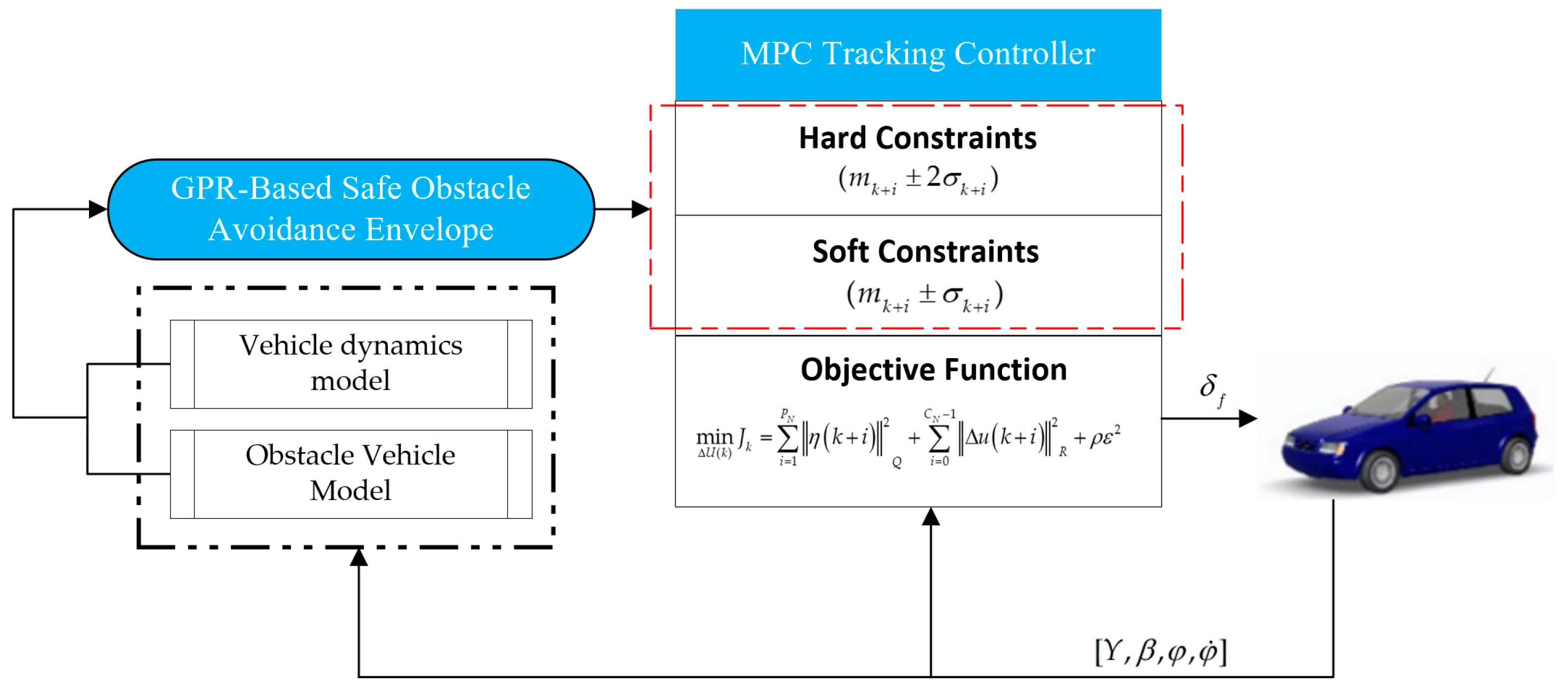
- A multi-objective MPC controller incorporating the safety obstacle avoidance envelopes as constraints is proposed. With soft and hard constraints imposed, the MPC controller solves the optimization problem, with vehicle stability and steering smoothness as the objectives, to obtain control commands that guarantee collision-free obstacle avoidance, meanwhile maintaining a good level of vehicle stability and steering smoothness. The experiments prove that, in challenging and dynamic scenes, the stability of the vehicle is significantly improved under the premise of avoiding obstacles safely.
2. Methodology
2.1. Vehicle Models
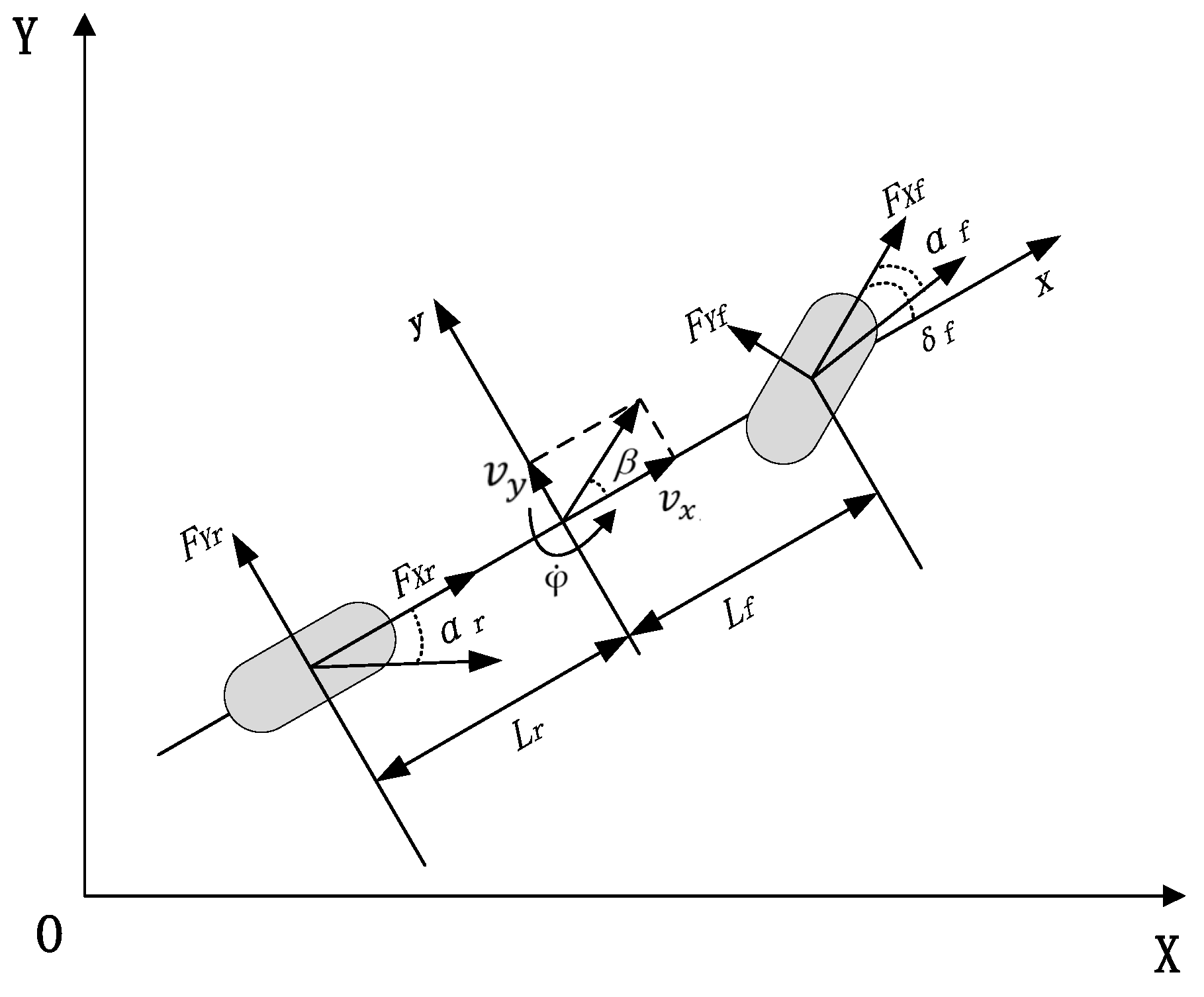
2.1.1. Ego-Vehicle Dynamics Model
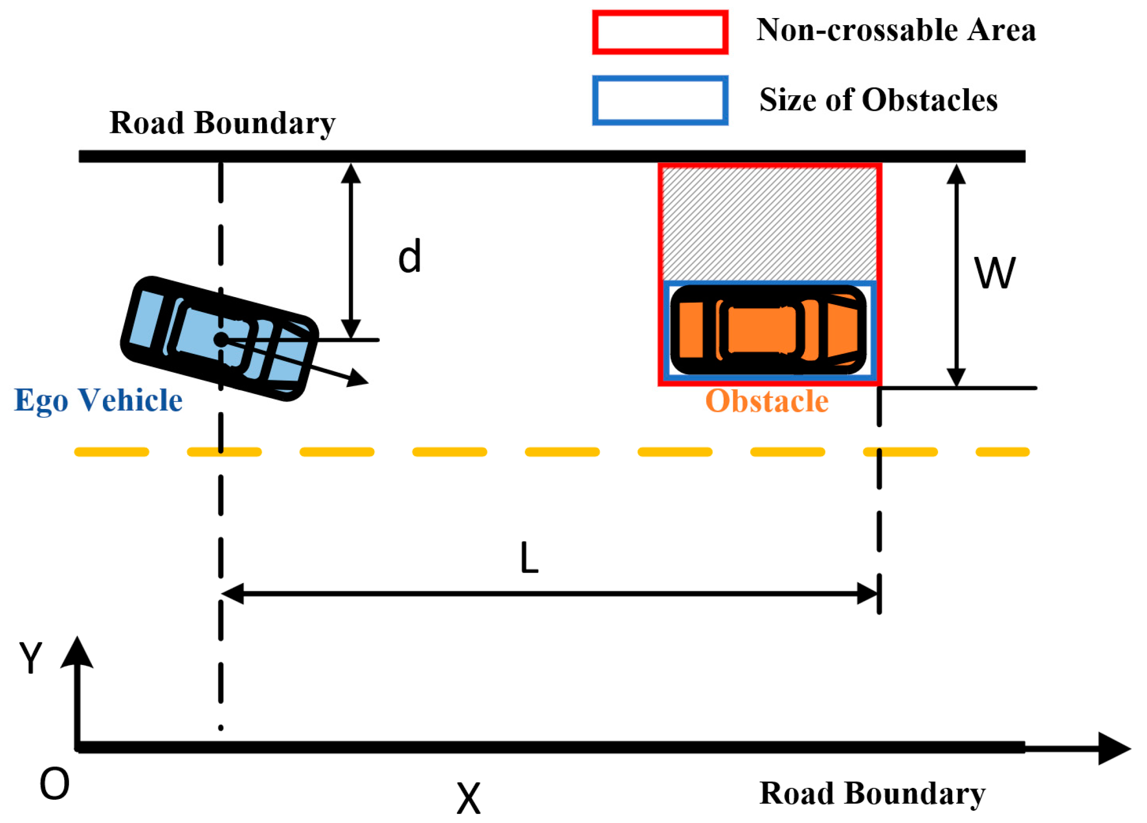
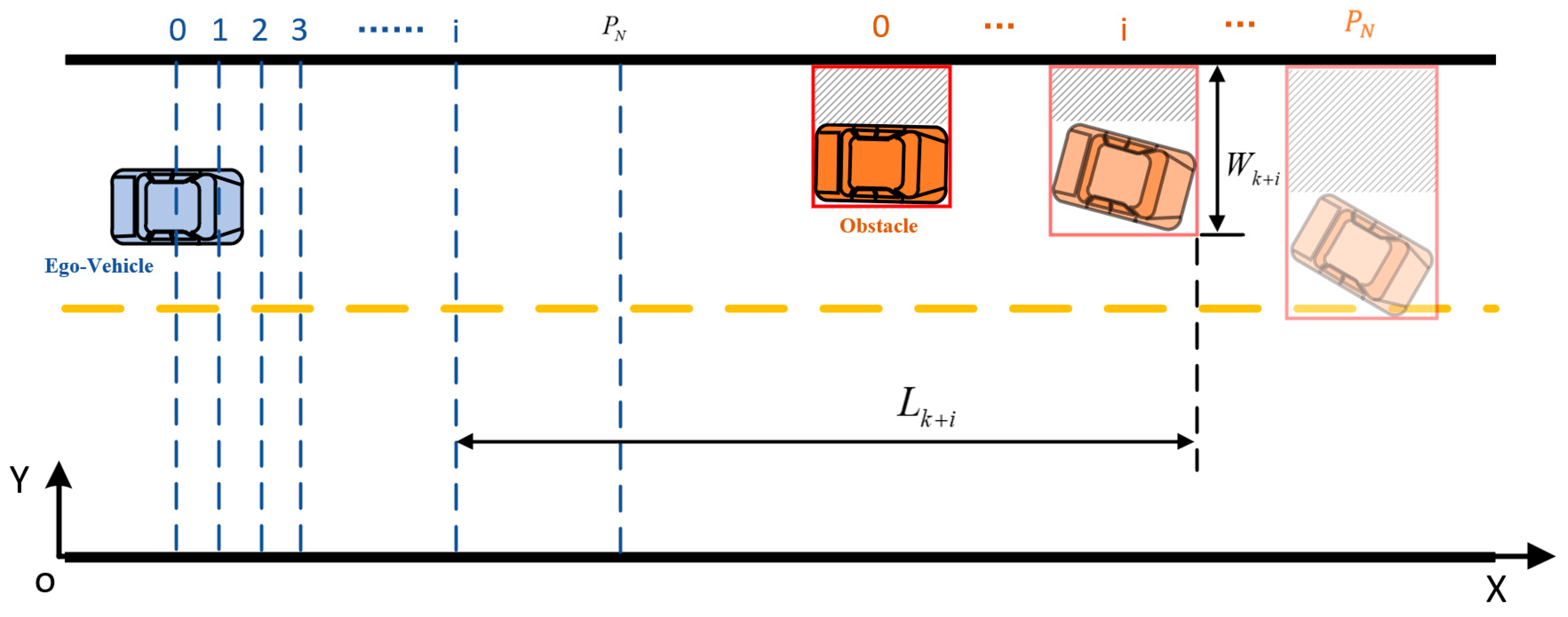
2.1.2. Obstacle Vehicle Model
2.2. GPR-Based Obstacle Avoidance Safety Envelope
2.3. Envelope-Based Obstacle Avoidance Tracking Controller
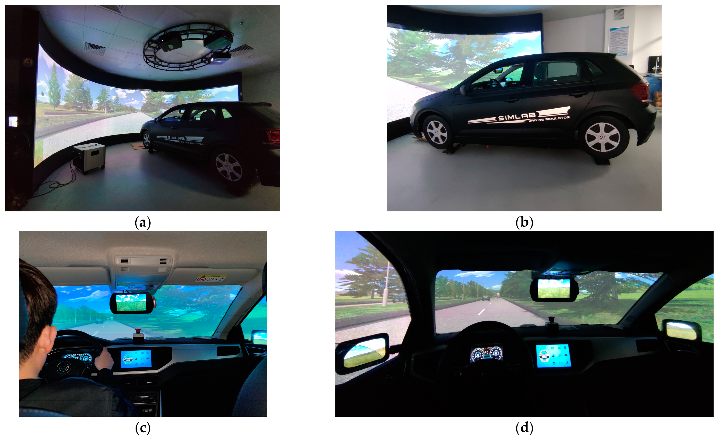
3. Experiments
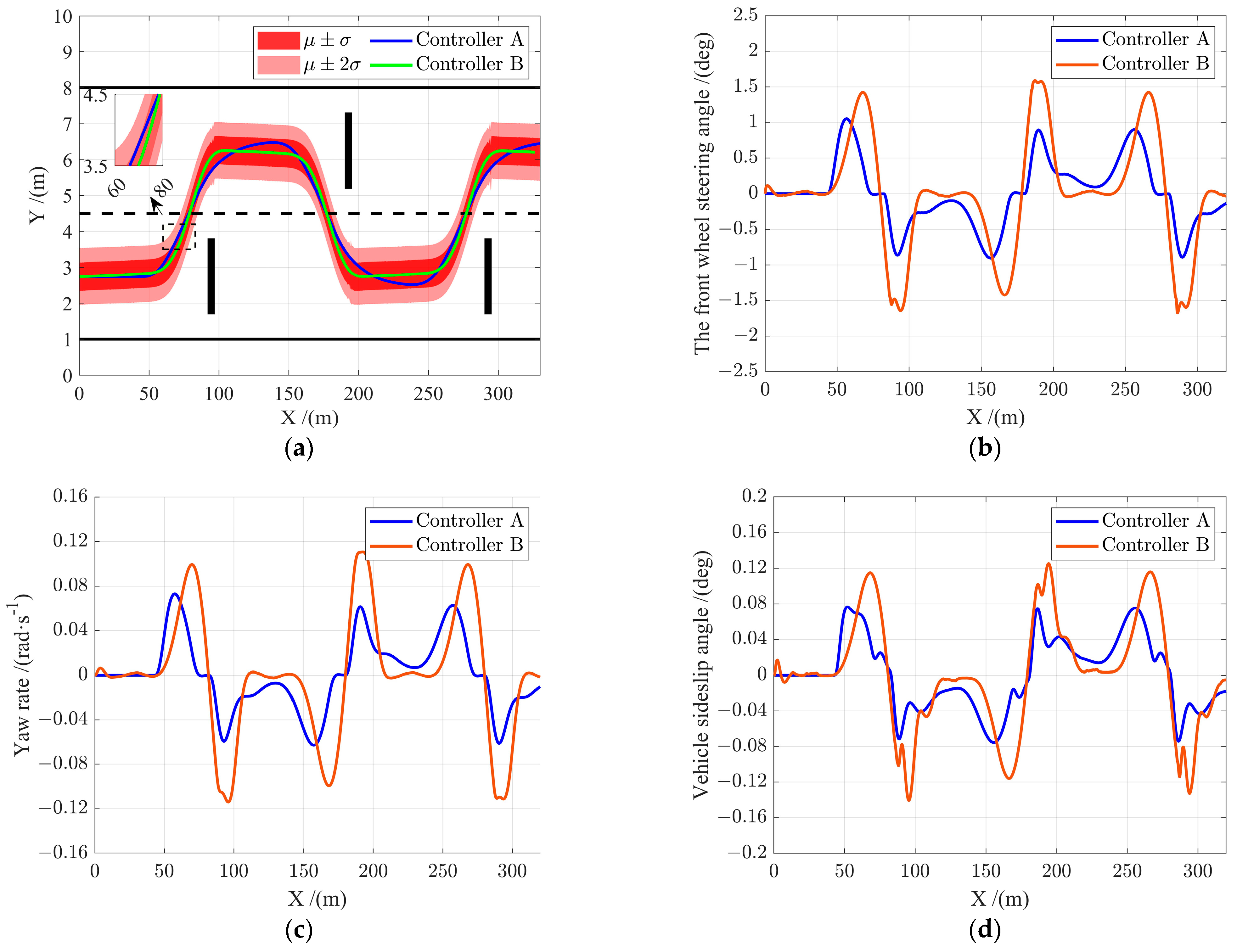
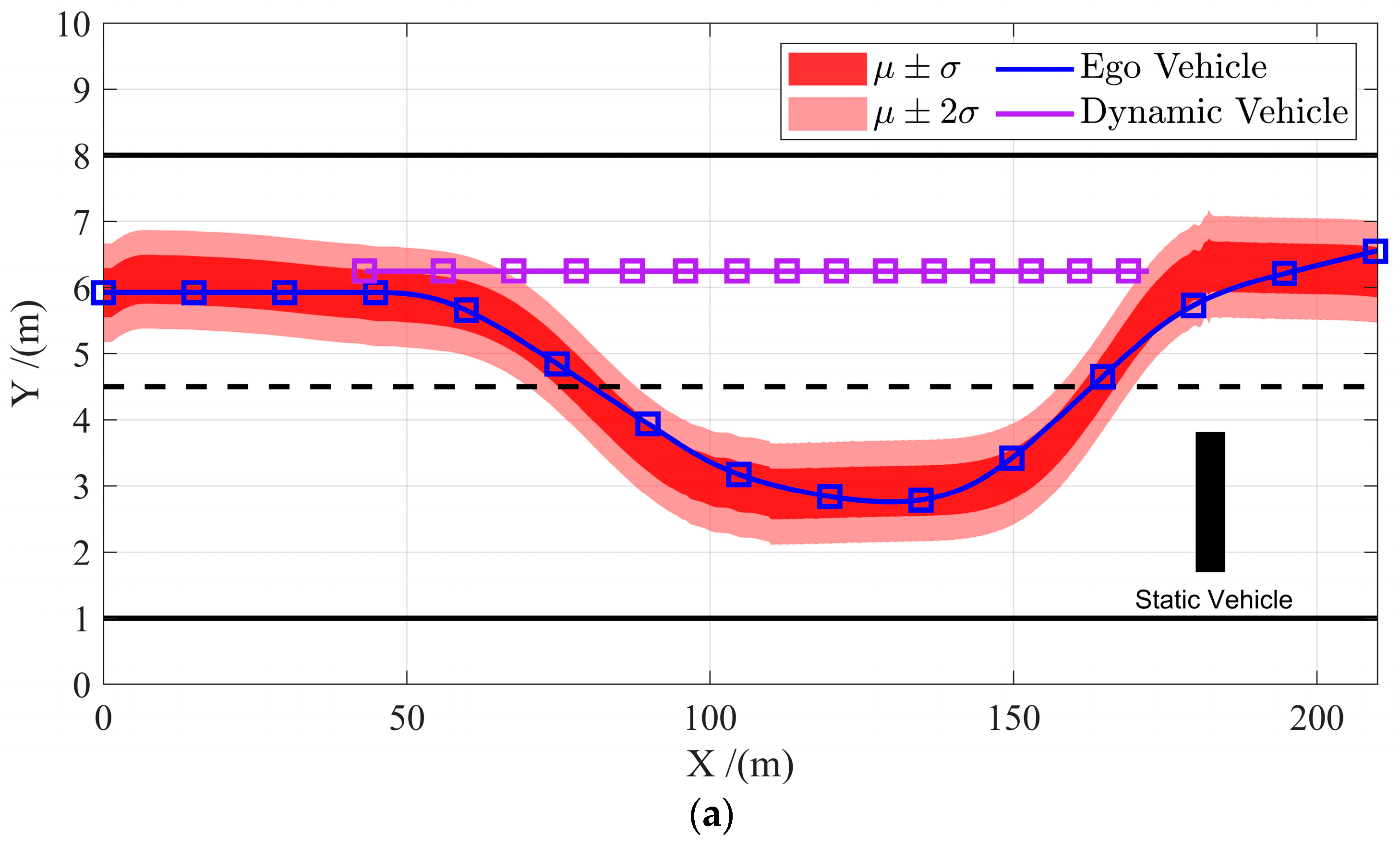
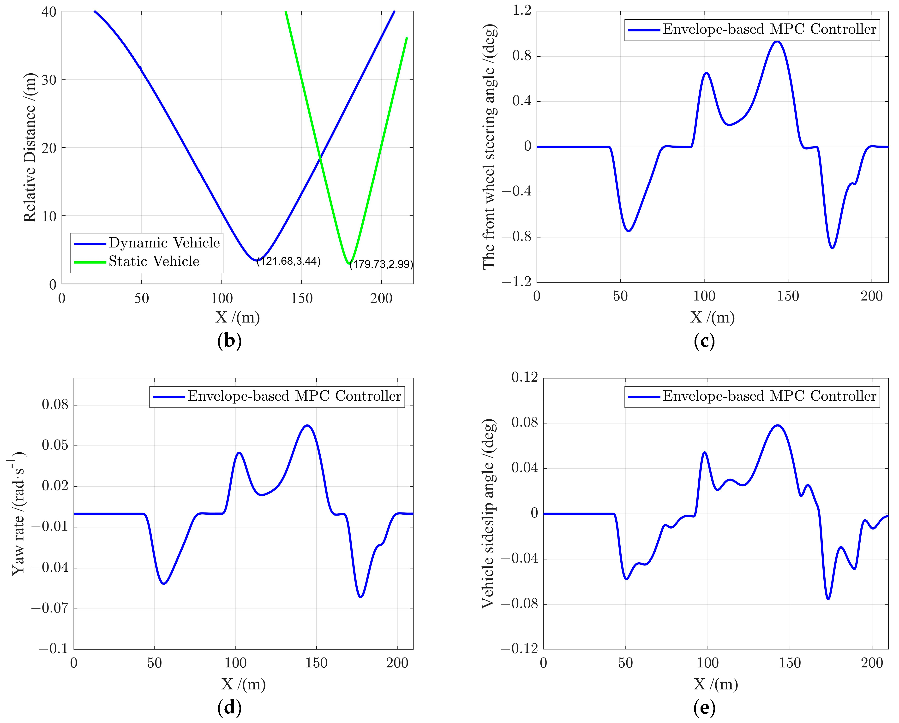
3.1. Scenario A
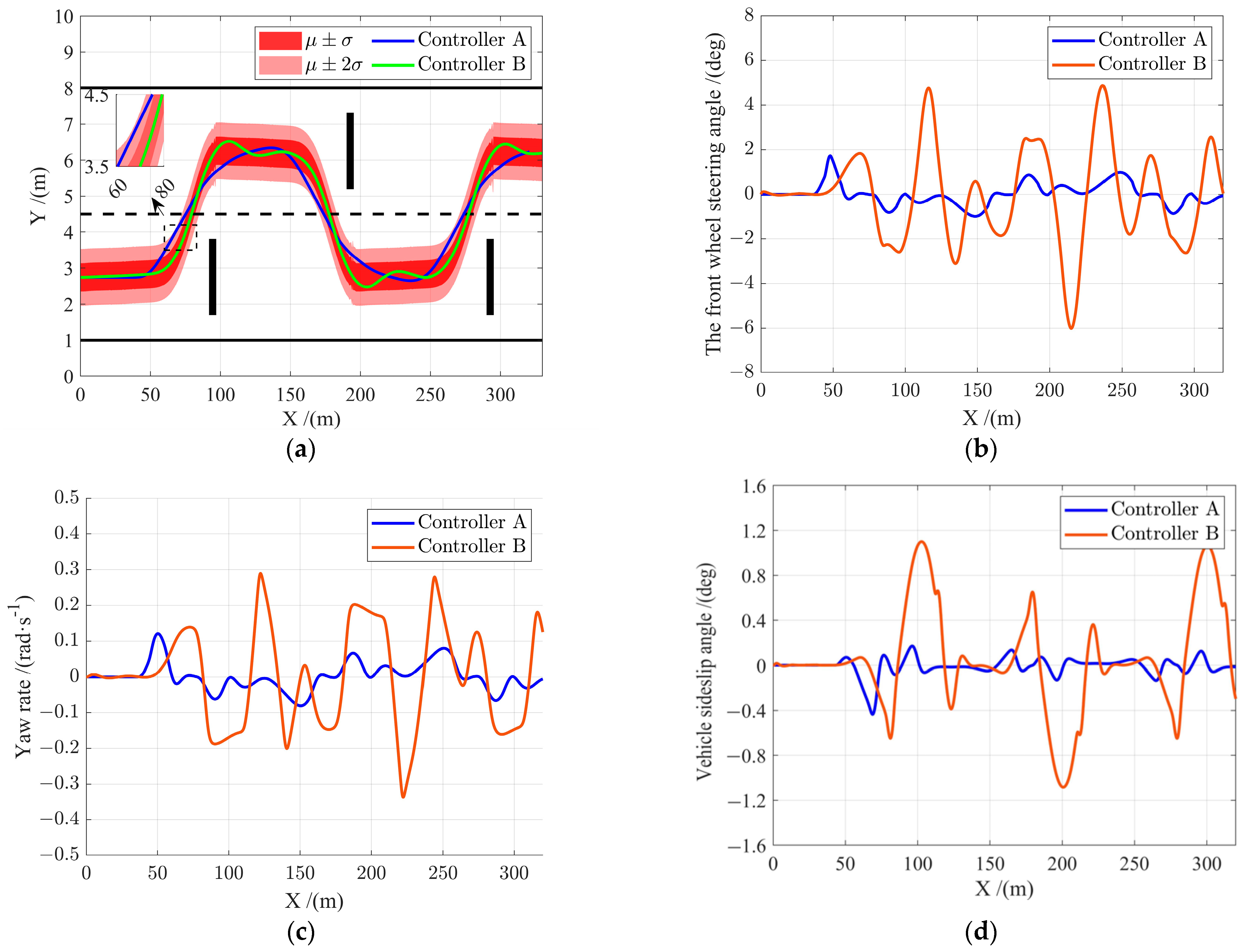
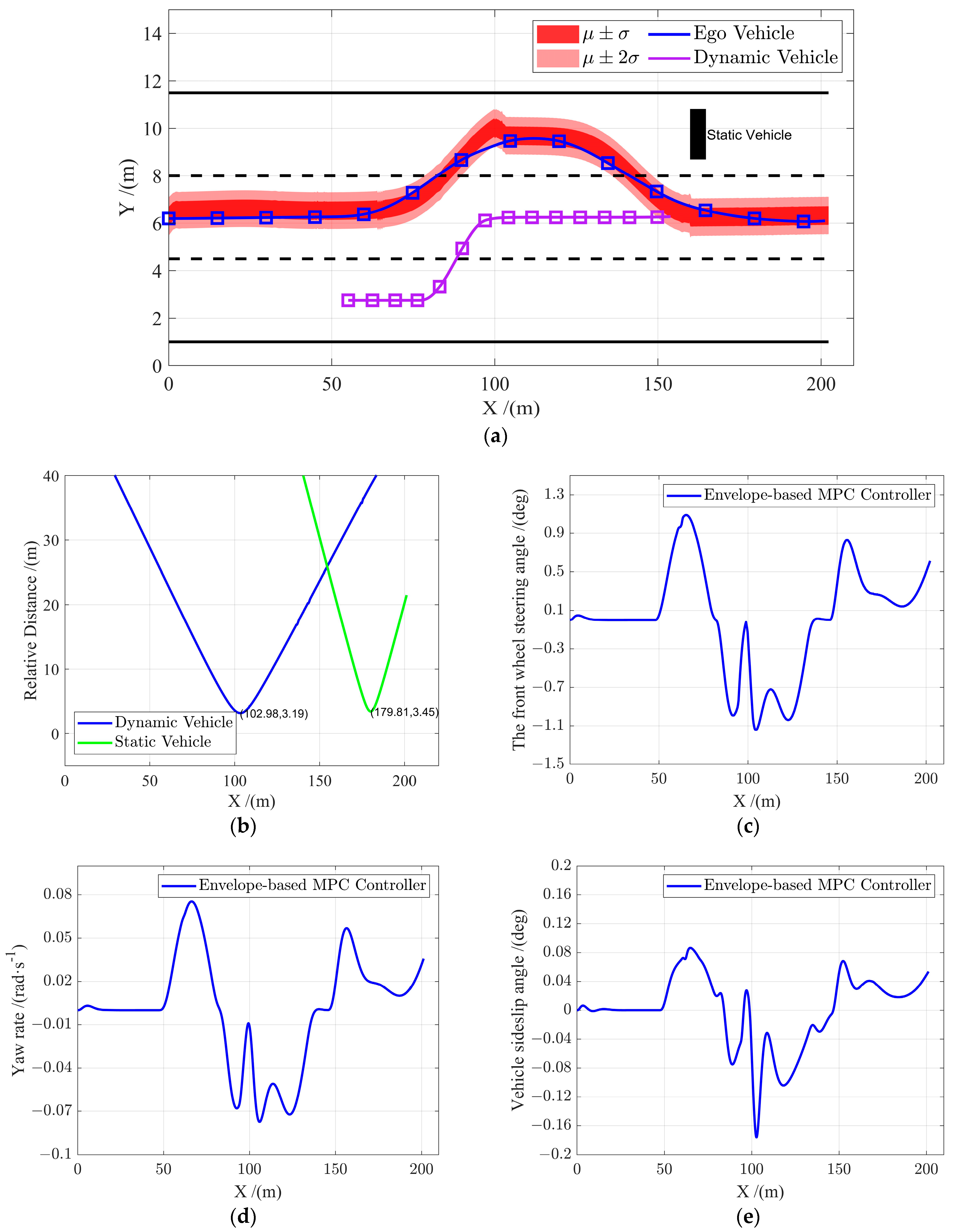
3.2. Scenario B
3.3. Scenario C
4. Conclusions
Author Contributions
Funding
Data Availability Statement
Conflicts of Interest
References
- Abbas, M.A.; Milman, R.; Eklund, J.M. Obstacle avoidance in real time with nonlinear model predictive control of autonomous vehicles. Can. J. Electr. Comput. Eng. 2017, 40, 12–22. [Google Scholar] [CrossRef]
- Maurer, M.; Gerdes, J.C.; Lenz, B.; Winner, H. Autonomous Driving: Technical, Legal and Social Aspects; Springer Nature: Cham, Switzerland, 2016. [Google Scholar]
- Jin, X.; Wang, J.; Yan, Z.; Xu, L.; Yin, G.; Chen, N. Robust vibration control for active suspension system of in-wheel-motor-driven electric vehicle via μ-synthesis methodology. J. Dyn. Syst. Meas. Control 2022, 144, 051007. [Google Scholar] [CrossRef]
- Jin, X.; Wang, J.; He, X.; Yan, Z.; Xu, L.; Wei, C.; Yin, G. Improving Vibration Performance of Electric Vehicles Based on In-Wheel Motor-Active Suspension System via Robust Finite Frequency Control. IEEE Trans. Intell. Transp. Syst. 2023, 24, 1631–1643. [Google Scholar] [CrossRef]
- He, S.; Wang, M.; Dai, S.-L.; Luo, F. Leader–follower formation control of USVs with prescribed performance and collision avoidance. IEEE Trans. Ind. Inform. 2018, 15, 572–581. [Google Scholar] [CrossRef]
- Sun, Q.; Guo, Y.; Fu, R.; Wang, C.; Yuan, W. Human-Like Obstacle Avoidance Trajectory Planning and Tracking Model for Autonomous Vehicles That Considers the Driver’s Operation Characteristics. Sensors 2020, 20, 4821. [Google Scholar] [CrossRef]
- Xie, Y.; Li, C.; Jing, H.; An, W.; Qin, J. Integrated Control for Path Tracking and Stability Based on the Model Predictive Control for Four-Wheel Independently Driven Electric Vehicles. Machines 2022, 10, 859. [Google Scholar] [CrossRef]
- Febbo, H.; Liu, J.; Jayakumar, P.; Stein, J.L.; Ersal, T. Moving obstacle avoidance for large, high-speed autonomous ground vehicles. In Proceedings of the 2017 American Control Conference (ACC), Seattle, WA, USA, 3 July 2017; pp. 5568–5573. [Google Scholar]
- Li, S.; Li, Z.; Yu, Z.; Zhang, B.; Zhang, N. Dynamic trajectory planning and tracking for autonomous vehicle with obstacle avoidance based on model predictive control. IEEE Access 2019, 7, 132074–132086. [Google Scholar] [CrossRef]
- Guo, H.; Shen, C.; Zhang, H.; Chen, H.; Jia, R. Simultaneous trajectory planning and tracking using an MPC method for cyber-physical systems: A case study of obstacle avoidance for an intelligent vehicle. IEEE Trans. Ind. Inform. 2018, 14, 4273–4283. [Google Scholar] [CrossRef]
- Li, X.; Sun, Z.; Cao, D.; Liu, D.; He, H. Development of a new integrated local trajectory planning and tracking control framework for autonomous ground vehicles. Mech. Syst. Signal Process. 2017, 87, 118–137. [Google Scholar] [CrossRef]
- Erlien, S.M.; Fujita, S.; Gerdes, J.C. Shared steering control using safe envelopes for obstacle avoidance and vehicle stability. IEEE Trans. Intell. Transp. Syst. 2015, 17, 441–451. [Google Scholar] [CrossRef]
- Brown, M.; Funke, J.; Erlien, S.; Gerdes, J.C. Safe driving envelopes for path tracking in autonomous vehicles. Control Eng. Pract. 2017, 61, 307–316. [Google Scholar] [CrossRef]
- Ryan, C.; Murphy, F.; Mullins, M. End-to-end autonomous driving risk analysis: A behavioural anomaly detection approach. IEEE Trans. Intell. Transp. Syst. 2020, 22, 1650–1662. [Google Scholar] [CrossRef]
- Wu, H.; Si, Z.; Li, Z. Trajectory tracking control for four-wheel independent drive intelligent vehicle based on model predictive control. IEEE Access 2020, 8, 73071–73081. [Google Scholar] [CrossRef]
- Albin, T.; Ritter, D.; Liberda, N.; Quirynen, R.; Diehl, M. In-vehicle realization of nonlinear MPC for gasoline two-stage turbocharging airpath control. IEEE Trans. Control Syst. Technol. 2017, 26, 1606–1618. [Google Scholar] [CrossRef]
- Suh, J.; Kim, B.; Yi, K. Design and evaluation of a driving mode decision algorithm for automated driving vehicle on a motorway. IFAC-PapersOnLine 2016, 49, 115–120. [Google Scholar] [CrossRef]
- Chen, S.; Chen, H.; Negrut, D. Implementation of MPC-Based trajectory tracking considering different fidelity vehicle models. J. Beijing Inst. Technol. 2020, 29, 303–316. [Google Scholar]
- Wei, S.; Zou, Y.; Zhang, X.; Zhang, T.; Li, X. An integrated longitudinal and lateral vehicle following control system with radar and vehicle-to-vehicle communication. IEEE Trans. Veh. Technol. 2019, 68, 1116–1127. [Google Scholar] [CrossRef]
- Chang, B.R.; Tsai, H.F.; Young, C.-P. Intelligent data fusion system for predicting vehicle collision warning using vision/GPS sensing. Expert Syst. Appl. 2010, 37, 2439–2450. [Google Scholar] [CrossRef]
- Nassi, B.; Mirsky, Y.; Nassi, D.; Ben-Netanel, R.; Drokin, O.; Elovici, Y. Phantom of the ADAS: Securing advanced driver-assistance systems from split-second phantom attacks. In Proceedings of the 2020 ACM SIGSAC Conference on Computer and Communications Security, Virtual, 9–13 November 2020; pp. 293–308. [Google Scholar]
- Schulz, E.; Speekenbrink, M.; Krause, A. A tutorial on Gaussian process regression: Modelling, exploring, and exploiting functions. J. Math. Psychol. 2018, 85, 1–16. [Google Scholar] [CrossRef]
- Goli, S.A.; Far, B.H.; Fapojuwo, A.O. Vehicle Trajectory Prediction with Gaussian Process Regression in Connected Vehicle Environment $\star$. In Proceedings of the 2018 IEEE Intelligent Vehicles Symposium (IV), Changshu, China, 26–30 June 2018; pp. 550–555. [Google Scholar]
- Williams, C.K.; Rasmussen, C.E. Gaussian Processes for Machine Learning; MIT Press: Cambridge, MA, USA, 2006; Volume 2. [Google Scholar]
- Li, Z.; Zhao, P.; Jiang, C.; Huang, W.; Liang, H. A Learning-Based Model Predictive Trajectory Planning Controller for Automated Driving in Unstructured Dynamic Environments. IEEE Trans. Veh. Technol. 2022, 71, 5944–5959. [Google Scholar] [CrossRef]
- Suh, S.H.; Bishop, A.B. Collision-avoidance trajectory planning using tube concept: Analysis and simulation. J. Robot. Syst. 1988, 5, 497–525. [Google Scholar] [CrossRef]
- Deisenroth, M.P. Efficient Reinforcement Learning Using Gaussian Processes; KIT Scientific Publishing: Karlsruhe, Germany, 2010; Volume 9. [Google Scholar]
- Kabzan, J.; Hewing, L.; Liniger, A.; Zeilinger, M.N. Learning-based model predictive control for autonomous racing. IEEE Robot. Autom. Lett. 2019, 4, 3363–3370. [Google Scholar] [CrossRef] [Green Version]
- Ryan, C.; Murphy, F.; Mullins, M. Semiautonomous vehicle risk analysis: A telematics-based anomaly detection approach. Risk Anal. 2019, 39, 1125–1140. [Google Scholar] [CrossRef] [PubMed]
- Wang, H.; Liu, B.; Ping, X.; An, Q. Path tracking control for autonomous vehicles based on an improved MPC. IEEE Access 2019, 7, 161064–161073. [Google Scholar] [CrossRef]


| Description | Symbol |
|---|---|
| Vehicle Mass | m |
| Distance from the center of mass to the front/rear axis | / |
| Longitudinal force of the front/rear tires | / |
| Lateral force of front/rear tires | |
| Sideslip angle of front/rear tires | |
| Steering angle of the front wheel | |
| Longitudinal/Lateral speed | |
| Yaw rate | |
| Sideslip Angle |
| Symbol | Value |
|---|---|
| m | 1723 kg |
| 4175 kg⋅ | |
| 1230 mm | |
| 1470 mm | |
| 62,700 N⋅ | |
| 66,900 N⋅ |
| Symbol | Value |
|---|---|
| T | 0.02 |
| 20 | |
| 5 | |
| Q | |
| R | 50000 |
| 1000 |
Disclaimer/Publisher’s Note: The statements, opinions and data contained in all publications are solely those of the individual author(s) and contributor(s) and not of MDPI and/or the editor(s). MDPI and/or the editor(s) disclaim responsibility for any injury to people or property resulting from any ideas, methods, instructions or products referred to in the content. |
© 2023 by the authors. Licensee MDPI, Basel, Switzerland. This article is an open access article distributed under the terms and conditions of the Creative Commons Attribution (CC BY) license (https://creativecommons.org/licenses/by/4.0/).
Share and Cite
Li, K.; Yin, Z.; Ba, Y.; Yang, Y.; Kuang, Y.; Sun, E. An Integrated Obstacle Avoidance Controller Based on Scene-Adaptive Safety Envelopes. Machines 2023, 11, 303. https://doi.org/10.3390/machines11020303
Li K, Yin Z, Ba Y, Yang Y, Kuang Y, Sun E. An Integrated Obstacle Avoidance Controller Based on Scene-Adaptive Safety Envelopes. Machines. 2023; 11(2):303. https://doi.org/10.3390/machines11020303
Chicago/Turabian StyleLi, Kang, Zhishuai Yin, Yuanxin Ba, Yue Yang, Yuanhao Kuang, and Erqian Sun. 2023. "An Integrated Obstacle Avoidance Controller Based on Scene-Adaptive Safety Envelopes" Machines 11, no. 2: 303. https://doi.org/10.3390/machines11020303