Article

Integrated Adhesion Coefficient Estimation of 3D Road Surfaces Based on Dimensionless Data-Driven Tire Model

1
Department of Mechanical Engineering, Shijiazhuang Tiedao University, Shijiazhuang 050043, China
2
State Key Laboratory of Mechanical Behavior in Traffic Engineering Structure and System Safety, Shijiazhuang Tiedao University, Shijiazhuang 050043, China
3
Department of Information Science and Technology, Shijiazhuang Tiedao University, Shijiazhuang 050043, China
*
Author to whom correspondence should be addressed.
Machines 2023, 11(2), 189; https://doi.org/10.3390/machines11020189
Submission received: 17 December 2022 / Revised: 27 January 2023 / Accepted: 28 January 2023 / Published: 31 January 2023
(This article belongs to the Special Issue Advanced Modeling, Analysis and Control for Electrified Vehicles)

Abstract

:
The tire/road peak friction coefficient (TRPFC) is the core parameter of vehicle stability control, and its estimation accuracy significantly affects the control effect of active vehicle safety. To estimate the peak adhesion coefficient accurately, a new method for the comprehensive adhesion coefficient of three-dimensional pavement based on a dimensionless data-driven tire model is proposed. Firstly, in order to accurately describe the contact state between the three-dimensional road surface and the tire during driving, stress distribution and multi-point contact are introduced into the vertical dynamic model and a new tire model driven by dimensionless data is established based on the normalization method. Secondly, the real-time assessment of lateral and longitudinal adhesion coefficients of three-dimensional pavement is realized with the unscented Kalman filter (UKF). Finally, according to the coupling relationship between the longitudinal tire adhesion coefficient and the lateral tire adhesion coefficient, a fuzzy reasoning strategy of fusing the longitudinal tire adhesion coefficient and the lateral tire adhesion coefficient is designed. The results of vehicle tests prove that the method proposed in this paper can estimate the peak adhesion coefficient of pavement quickly and accurately.

1. Introduction

The rapid increase in the number of cars also brings about frequent traffic accidents and other problems [1,2]. On one hand, these traffic accidents are caused by drivers, such as drunk driving, fatigue driving, non-professional factors, etc. On the other hand is the traffic accident caused by the change in tire performance due to changes in climate and road conditions. For example, under severe winter ice and snow weather conditions, the road surface becomes slicker and the TRPFC between the three-dimensional road surface and the tire is reduced, making the vehicle more prone to collision, sideslip, and other accidents. The state change between tire/road poses a higher challenge to the active safety control strategy of autonomous vehicles [3,4,5]. Especially under complex working conditions such as heavy load, high speed, braking, and emergency steering, the contact between the three-dimensional road surface and the tire is in a non-linear, transient, and non-smooth dynamic action process. The dynamic frictional contact relationship between the three-dimensional road surface and the tire is complex. Suppose the active control strategy only relies on the front-end sensing sensors to obtain the surrounding vehicle information and the traditional static adhesion coefficient; in that case, it cannot meet the demand for autonomous vehicles in full road driving conditions. Therefore, the research on how to describe the tire/road contact state and estimate the TRPFC timely and accurately in the vehicle driving process has become a complex problem in the area of active vehicle control.
Many studies have been done nationally and internationally on the estimation of TRPFC, which can be categorized into cause-based and effect-based [6].
The cause-based method mainly uses optical sensors, acoustic sensors, tire tread sensors, etc. to measure parameters related to road friction and estimate the TRPFC.
In Ref. [7], a real-time acoustic analysis algorithm based on tire/road noise is proposed to classify asphalt state. In [8,9], TRPFC is estimated by measuring the degree of light absorption and scattering by road surface with an optical sensor. In Ref. [10], sensors are used to extract texture features and color grades of roads to complete road classification. In [11], the correlation between road state and intelligent tire test signal is established through the acceleration signal of the intelligent tire to complete the classification and identification of pavement. In [12], TRPFC is estimated by measuring the lateral strain of the tire part using piezoelectric sensors arranged in the tire. In [13], the triaxial acceleration sensor is installed on the ridge line inside the tire for data acquisition, and the vertical load of the tire is obtained by neural network algorithm. In Refs. [14,15], the triaxial acceleration sensor installed in the tire is used to collect the vertical acceleration signal, and it is used as the index of road friction. The test roads are ice and cement, respectively. The results show that the vibration characteristics caused by sliding on the low friction road surface can be used to identify the adhesion state of the road.
The advantage of the above identification method is that it can better identify the TRPFC when the tire’s longitudinal force is small. However, this method is challenging to popularize and apply, mainly for the following reasons. Firstly, because vehicles’ actual running road conditions are complex and changeable, road surface recognition based on acoustic and optical sensors needs a lot of data processing and training. Secondly, the tread sensor-based method needs to arrange the sensor within the tire, which places higher demands on the power supply and reliability of the detector.
The effect-based method estimates the TRPFC by measuring and analyzing the response of the whole vehicle caused by the road surface change. The identification method estimates the TRPFC based on a mathematical model, primarily including the dynamic model-based estimation method and the curve-based estimation method of the coefficient-of-slip ratio of road adhesion.
In [16], the recursive least squares (RLS) method is applied to estimate the slip and slope of test vehicles on icy pavement and dry asphalt pavement, respectively. The results demonstrate that this method can rapidly and reliably identify adhesion coefficients of different pavements. In [17], on the basis of the connection between both the slip ratio and adhesion coefficient, in order to estimate the coating adhesion coefficient, we adopt the least square method for multivariate fitting. A longitudinal logistic model of vehicle collision avoidance is designed to consider the gradient of the road and the road adherence coefficient. In [18], the wheel slip rate and the adhesion coefficient are used as the input parameters of fuzzy logic, and then the adhesion coefficient of the current road surface is finally estimated. In [19], an estimation algorithm of the TRPFC based on mixed theory is proposed. In the range of small slip ratio, the generalized regression neural network theory is used to accurately create the mapping between input parameters and the pavement adhesion coefficient. In contrast, in the range of large slip ratio, the magic tire pavement model combined with Bayesian theory is used for estimation. In [20,21,22], a method for identifying the TRPFC under longitudinal sliding conditions of tires establishes the relationship between longitudinal tire force and sliding rate through tire models such as the Burckhardt and Dugoff models. In summary, the advantage of this kind of algorithm is that it does not need expensive sensors. However, it only uses low-cost sensors (such as wheel speed sensors, combined sensors, etc.), and this method has fast response speed and high estimation accuracy.
As can be seen, researchers have made numerous accomplishments in TRPFC estimation. However, many problems still need to be addressed.
Firstly, the existing estimation methods of the TRPFC based on vehicle dynamics pay little attention to road roughness, and most give little consideration to road excitation or simplify it into a two-dimensional road non-uniformity model. These differences inevitably result in decreased accuracy of the TRPFC algorithm. Therefore, how to account for three-dimensional road roughness in the dynamic model and how to reduce model error are pressing problems that need to be addressed.
Secondly, the current research methods mainly focus on estimating vehicle longitudinal or lateral adhesion coefficients and seldom consider the coupling process of vehicle longitudinal or lateral motion. How to integrate longitudinal or lateral movements is also a vital issue.
Finally, tires are affected by many conditions during driving, and many scholars have studied this at present. In [23], finite element (FE) model techniques with particular applications of material properties accurately estimate the parameters of flexible ring tire models. In [24], The variation law between tire size contact area and pressure and load in summer was measured by experiments. In [25], a reliable three-dimensional (3D) tire-pavement interaction model is established to simulate the interface contact stress under static conditions. In [26], a tire sensing approach is used to investigate the rolling resistance force through measurements of the rolling deformation of truck tires. In [27], the vehicle accident is analyzed according to the tire yaw trace information deposited on the road surface. In [28,29], experiments under the condition of static load measure the data. The obtained results made it possible to determine the directional stiffness of the radial, peripheral, lateral, and torsional tires. In [30], by embedding the sensor into the tire, the tire force is estimated based on the acceleration signal. In [31], to solve the longitudinal and lateral tire force estimation of four-wheel drive vehicles, a robust PMI observer based on an LPV model is proposed. In [32], an integrated friction estimation algorithm based on a half-car vehicle model that can simultaneously estimate the combined friction condition along the longitudinal and lateral directions with some basic measurements is presented. In [33], an integrated tire-vehicle model is proposed to evaluate vehicle braking performance based on Persson’s friction theory, a tire hydroplaning finite element model, and a vehicle dynamic analysis.
In summary, the tire model has a fatal effect in estimating the adhesion coefficient. The current steady tire models can be categorized into theoretical models [34,35,36,37,38,39], empirical models [40,41], and semi-empirical models [42,43,44,45]. However, most of the formulas of the tire models mentioned above are complex, requiring many parameters, and solving speed are slow, which is challenging to meet real-time control requirements. Furthermore, most algorithms are based on the tire model with fixed parameters. However, the tire model is non-fixed parameter in actual working conditions. How to build a tire model with no parameters and adaptive changes with the vehicle’s driving state is particularly important.
The main aims of this study are to address the above issues.
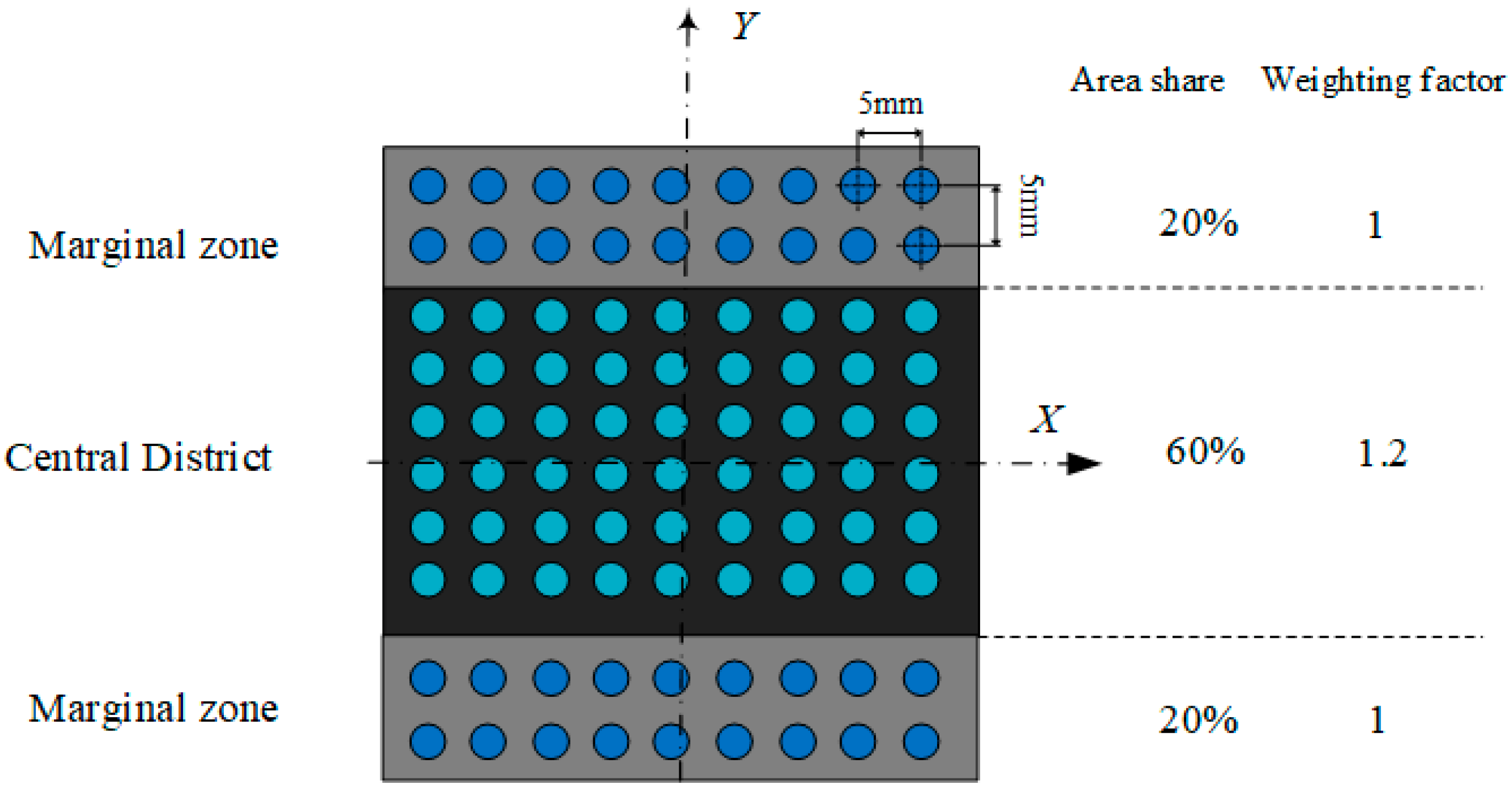
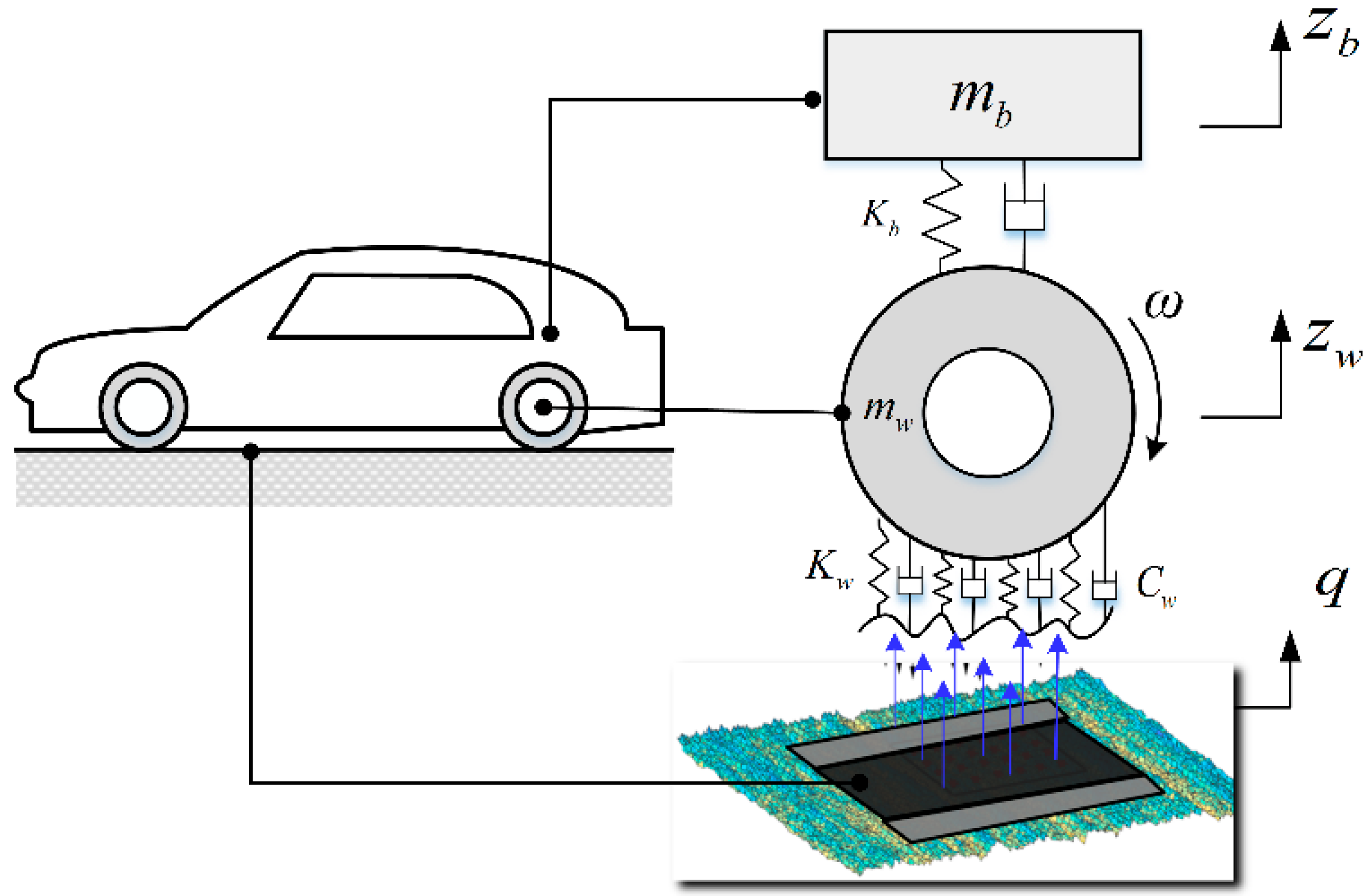
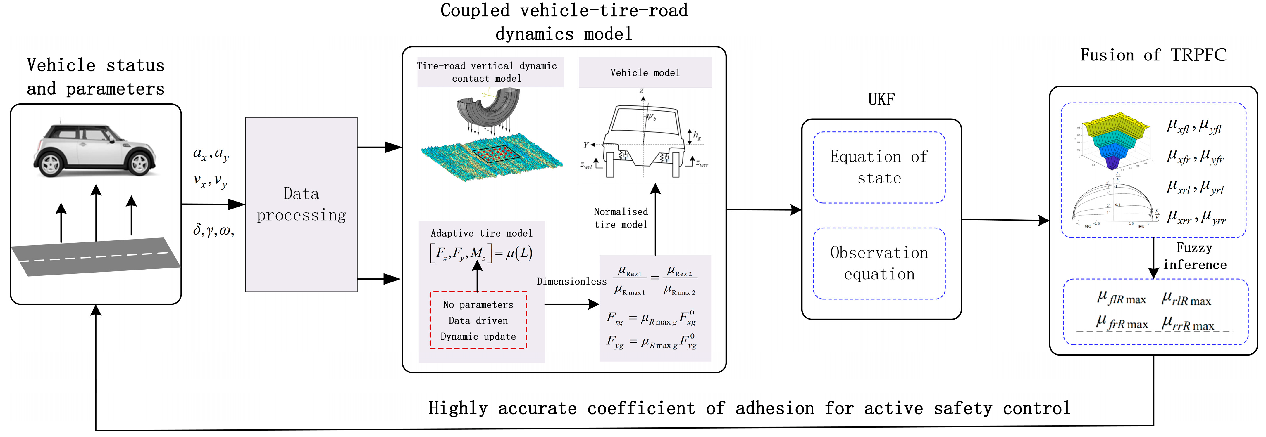
  • To describe the pavement excitation more accurately, the stress distribution pattern between the tire/road and the mechanical properties of the multi-point contact are considered in the model of the vertical dynamics.
  • In order to address the parameter identification problem of the traditional tire model, a new dimensionless data-driven tire model is proposed to represent the dynamic friction relationship between the three-dimensional road surface and the tire.
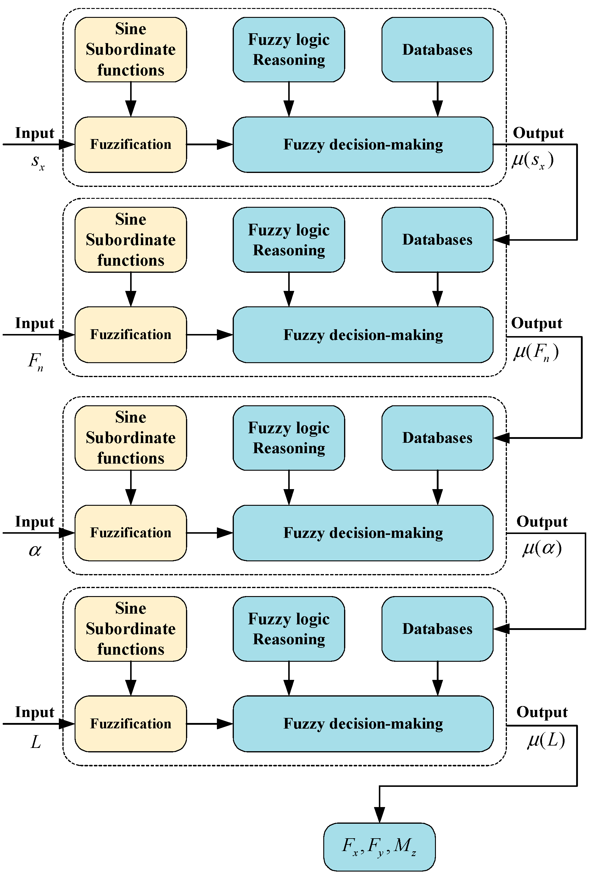
  • To estimate the integrated adhesion coefficients. According to the coupling relationship between the longitudinal and lateral adhesion coefficients, the fuzzy inference strategy is adopted to fuse the longitudinal tire adhesion coefficients and lateral tire adhesion coefficients obtained from the UKF algorithm.
The main structure of this article is as follows. Section 2 mainly introduces the establishment of the vehicle planar dynamics model and the vertical dynamic model. Section 3 mainly explains the algorithm of the peak adhesion coefficient. In Section 4 and Section 5, the effectiveness of this algorithm is verified by actual vehicles and simulated vehicles. Section 6 gives the conclusion of this paper.

2. Modeling of Vehicle/Tire/Road Interactions

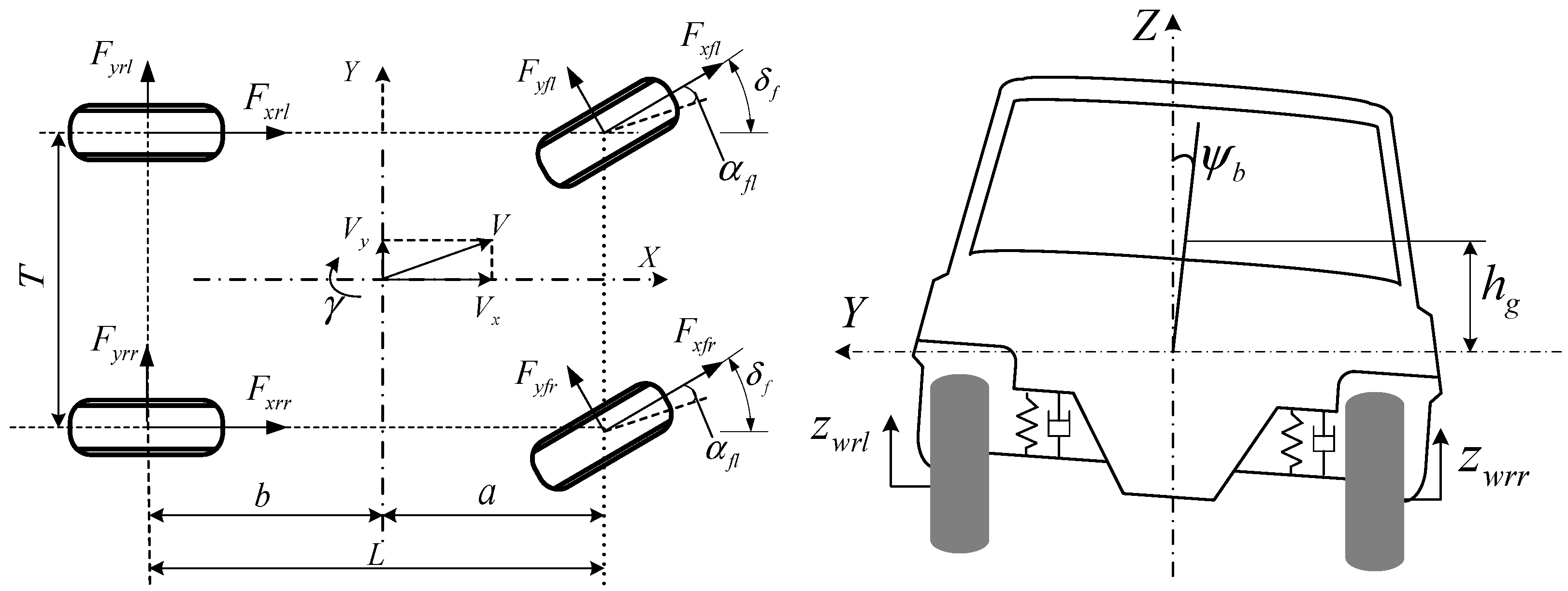
2.1. Vehicle Planar Dynamic Model

According to the research needs, the pitch, tire deformation, road slope, and aerodynamics are neglected, and the vehicle dynamics model is established based on the D’Alembert principle, and the suspension part is simplified to several springs and dampers, as shown in Figure 1.
The vehicle planar four-wheel dynamics models is as follows [46].
The longitudinal equation is as follows:
m z ( v ˙ x v y γ ) + m b z ˙ b θ ˙ b = F x f l cos δ f F y f l sin δ f + F x f r cos δ f + F x r r F y f r sin δ f + F x r l
The lateral equation is as follows:
m z ( v ˙ y + v x γ ) m b z ˙ b ψ ˙ b m b h g ψ ¨ b = F x f l sin δ f + F y f l cos δ f + F x f r sin δ f + F y r l + F y f r cos δ f + F y r r
The yaw equation is as follows:
γ ˙ I z + I x z ψ ¨ b = T 2 ( F x r r F y f r sin δ f + F x f r cos δ f ) b ( F y r r + F y r l ) T 2 ( F x f l cos δ f + F x r l F y f l sin δ f ) + a ( F y f l cos δ f + F x f r sin δ f + F x f l sin δ f + F y f r cos δ f )
where F x f l , F x f r , F x r l , F x r r are the tire force of longitudinal for four wheels, separately; F y f l , F y f r , F y r l , F y r r are the tire force of lateral for four wheels, separately; v x is longitudinal velocity; v y is lateral velocity. γ is yaw rate, ψ b is roll angle, δ f is front wheel steering angle, and θ b is pitch angle for the vehicle. G is 9.8   m / s 2 , a x is longitudinal for the vehicle and a y is lateral accelerations for the vehicle. I x z is the inertia product in the axle X and Z. α f l is slip angle for the left front wheel, α f r is the slip angle for the right front wheel. Table 1 provides the key parameters required by the vehicle in the vehicle dynamics model and test. Data are from Ref. [47].

2.2. Vertical Dynamic Model

The interaction between the three-dimensional road surface and tire is achieved through a small contact surface, and the contact area is one of the core factors determining the tire’s mechanical properties. As the length of the tire footprint changes when the tire rolls on the three-dimensional road, this paper uses the experimental method to measure the length of the tire footprint, as shown in Figure 2a. Most vehicles use radial tires, so this experiment takes radial tires as an example [48,49]. Under the standard tire pressure, increasing pressure is applied to the tires, and the tire footprints and lengths under different pressures are recorded [48,49], as shown in Figure 2b,c.
Linear fitting the data obtains a functional relationship [48,49], as shown in Formulas (4) and (5):
L = 0.006741 x + 80.786
S = 1.45825 x + 2215.2
where x is the vertical load (N); L is the grounding footprint length (mm); S is the ground footprint area (mm2).
According to the different distributions of contact stress on the contact surface, the contact surface is divided into different areas in this paper: the middle part is the central district, accounting for 60%, and the rest is the marginal area, accounting for 40%, as shown in Figure 3. According to the experimental measurement [50], the average contact stress ratio between the center area and the edge area of the radial tire is about 1.2 to determine the weighting coefficient of each area.
Based on fractal theory [40], the 3D pavement surface is reconstructed and used as a spatial excitation for vehicle systems. The vertical load determines the contact area between the tire/road applied to the tire, as shown in Equation (5). According to the stress distribution law, the actual contact surface is divided into three areas: a central area and two edge areas. To balance the calculation efficiency and retain the integrity of the pavement features, the lateral and longitudinal distances between adjacent point units are both 5mm, where the weighting factor of the discrete point unit in the edge area is 1, and that of the discrete point unit in the central district is 1.2. The established 3D pavement excitation is transferred into the vertical dynamic contact models, as shown in Figure 4.
The tire and three-dimensional road dynamic contact model is as follows:
m w z ¨ w + C b ( z ˙ w z ˙ b ) + K b ( z w z b ) + i = 1 m c w i ( z ˙ w i q ˙ i ) + i = 1 m k w i ( z w i q i ) + 1.2 j = 1 n c w i ( z ˙ w i q ˙ i ) + 1.2 j = 1 n k w i ( z w i q i ) = 0 m b z ¨ b + C b ( z ˙ b z ˙ w ) + K b ( z b z w ) = 0
k w i = K w n + m c w i = C w n + m
The load for each wheel is:
F z f l = b 2 L m z g b h g L B m b a y m b a x h g 2 L + k ψ ψ b + i = 1 m k w f ( z w f l q f l ) + 1.2 j = 1 n k w i ( z w f l q f l )
F z f r = b 2 L m z g + b h g L B m b a y m b a x h g 2 L + k ψ ψ b + i = 1 m k w f r ( z w f r q f r ) + 1.2 j = 1 n k w f r ( z w f r q f r )
F z r l = a 2 L m z g a h g L B m b a y + m b a x h g 2 L + k ψ ψ b + i = 1 m k w r l ( z w r l q r l ) + 1.2 j = 1 n k w r l ( z w r l q r l )
F z r r = a 2 L m z g + a h g L B m b a y + m b a x h g 2 L + k ψ ψ b + i = 1 m k w r r ( z w r r q r r ) + 1.2 j = 1 n k w r r ( z w r r q r r )
where m and n are the number of contact points in the marginal area and central district; k w i , K w , and K b are the tire distribution stiffness factor, tire stiffness factor, and suspension stiffness factor, respectively; c w i , c b , and c w are the tire distribution damping factor, suspension damping factor, and tire damping factor, respectively. q i ( i = f l ,   r r ,   r l ,   f r ) indicates the road roughness. z w i ( i = r l ,   r r ,   f l ,   f r ) indicates vertical displacement for the centroid, separately. Table 1 shows the key parameters for the vehicle dynamics models.

2.3. Adaptive Parameter-Free Tire Model Based on Data Driven

In this section, a new intelligent tire model is put forward. This model has no complicated formula form, and it does not need a lot of experimental fitting of the coefficients. It only needs to input the dynamic parameter variables of the vehicle in the running process to get the mechanical characteristics between the tire and the road. Because the slip ratio, vertical load, inclination angle, and the length of the footprint have great influence on the mechanical properties of the tire, the fuzzy tire model uses the above parameters to obtain the final mechanical properties of the tire.

2.3.1. Tire Model

There are four layers of fuzzy operating systems in the model, as shown in Figure 5, each containing two parts: fuzzification and fuzzy decision. Fuzzification is to fuzzify the dynamic input parameters with the sine membership function, convert them into recognizable fuzzy language values, and then send them to the next fuzzy decision-making part. The decision-making process is divided into fuzzy logic reasoning and database. Fuzzy reasoning contains corresponding fuzzy operation rules, and Formulas (12)–(16) are specific operation processes; the required data for the fuzzy operation rules of the database are provided, and the data after the decision are output as the database of the lower system.
The detailed expressions in the first level of fuzzy operations are shown in Equation (12)
μ S x = i = 1 n B 1 S x , F n , α , L M i , 1 ( S x )
where μ S x is the data input to the lower level, and B 1 S x , F n , α , L is the data from the Ref. [51], obtained by fitting in the LuGree model, and   M i , 1 S x is the fuzzy set of slip rates.
The detailed expression in the second level of fuzzy operations is shown in Equation (13)
μ F n = i = 1 n B 2 F n , α , L M i , 2 ( F n ) , B 2 F n , α , L = μ S x  
where μ F n is the data input to the lower layer, B 2 F n , α , L is the experimental data obtained from the system in the upper layer, and   M i , 2 F n is the fuzzy set of vertical loads.
The detailed expression in the third level of fuzzy operations is shown in Equation (14).
μ α = i = 1 n B 3 α , L M i , 3 ( α ) , B 3 α , L = μ F n  
where μ α is the data input to the lower layer, B 3 α , L is the experimental data obtained from the system in the upper layer, and M i , 3 ( α ) is the fuzzy set of angles.
The detailed expression in the fourth level of fuzzy operations is shown in Equation (15).
μ L = i = 1 n B 4 L M i , 4 ( L ) , B 4 L = μ α
where μ L is the final output, and B 4 L is the experimental data obtained from the system in the upper layer, and M i , 4 ( L ) is the fuzzy set of contact line lengths.
The final output is shown in Equation (16)
F x , F y , M z = μ L
Tire longitudinal forces, lateral forces, and aligning torque can be gained by inputting the appropriate dynamic parameters to each system layer. The data can be driven online and updated in real time. The model proposed in this section requires only a small amount of data to be driven, avoiding the effect of parameters on the physical characteristics of the tire in existing models.

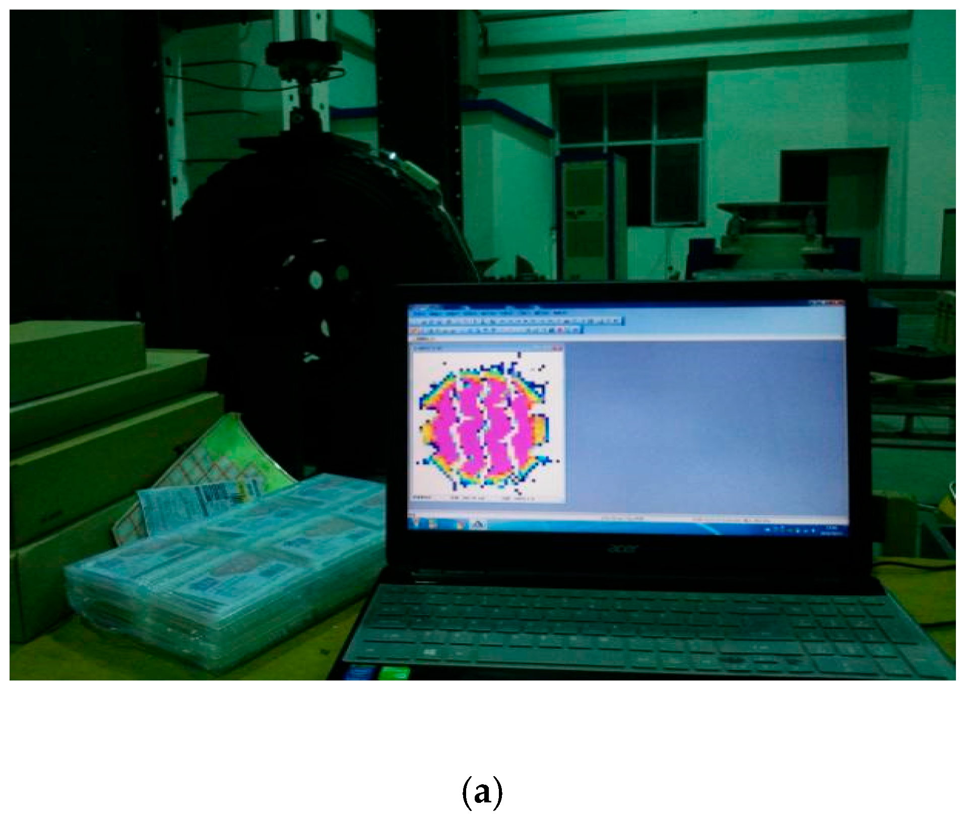
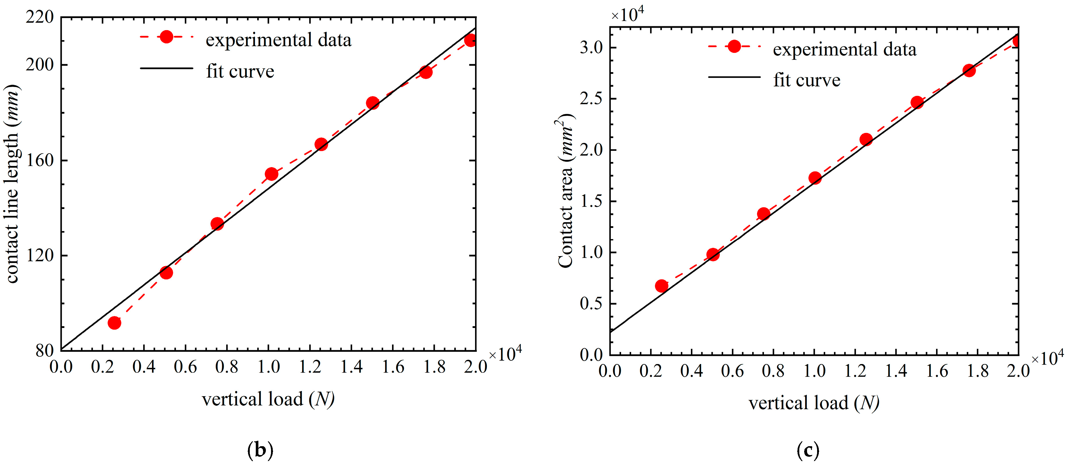
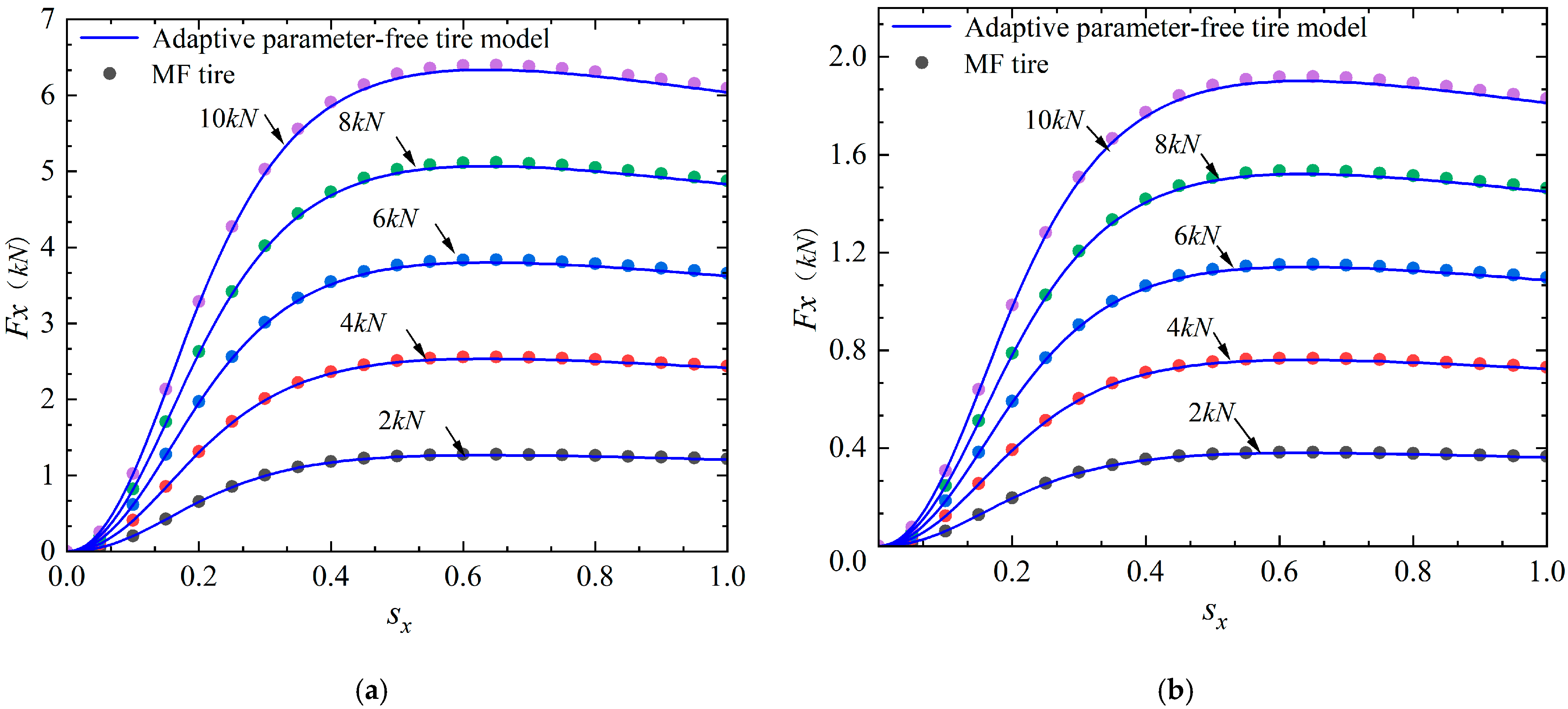
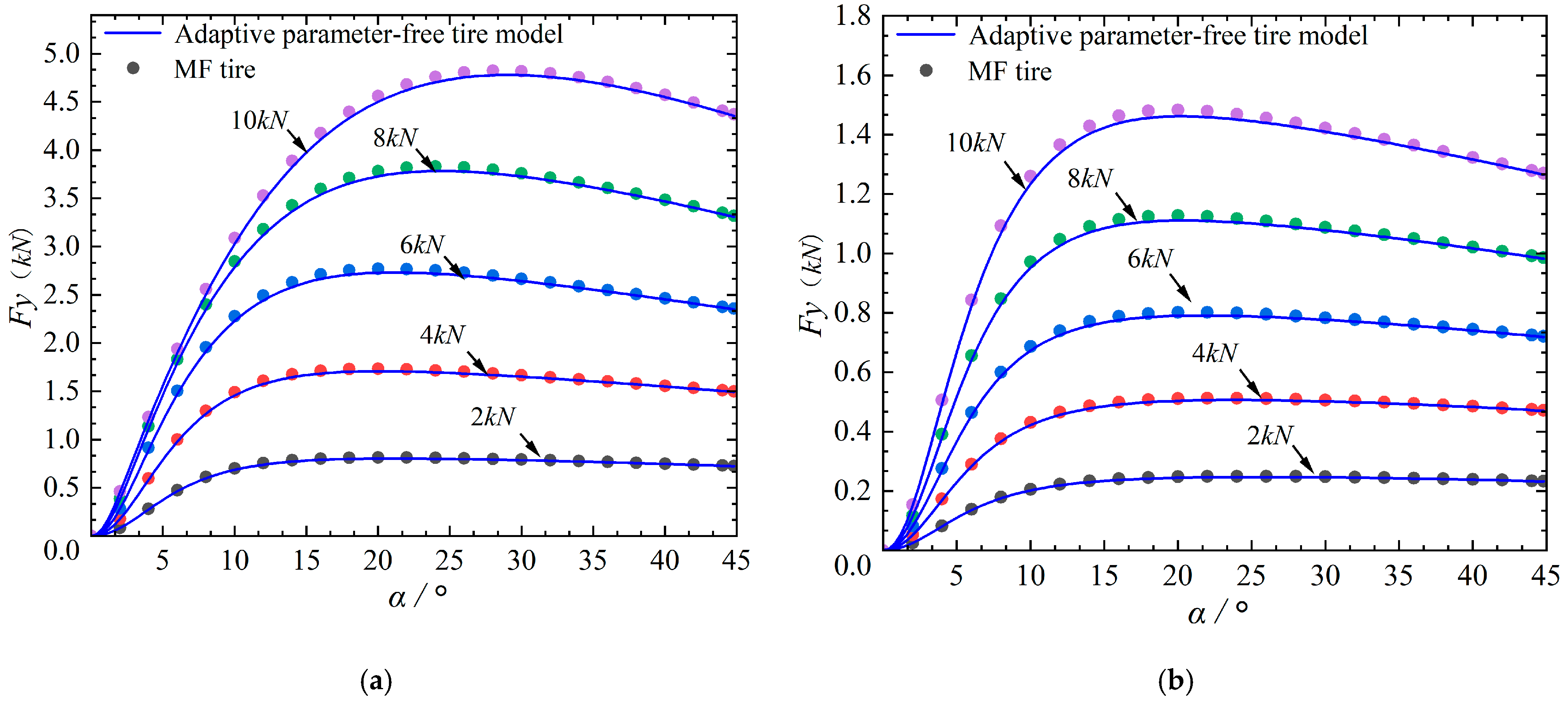
2.3.2. Tire Model Verification

The MF tire model has been widely used in vehicle dynamics simulation and analysis because of its high fitting accuracy and wide application range. Therefore, the magic tire is selected as the comparative data in this paper, and the magic formula and parameters are from Ref. [51].
Figure 6 verifies longitudinal tire force and compares the tire force of two tire models under compound slip conditions.
Comparing the two data groups with the root mean square error result, the root mean square is Formula (17), and its RRMSE value is less than 0.0954.
R R M S E = 1 n i = 1 n x s i x e i x e i 2
where x s i is adaptive tire model data, x e i is MF tire model data.
Figure 7 verifies tire lateral force and compares the tire force of two tire models under compound slip conditions.
Comparing the two groups of data with the root mean square error result, the RRMSE value is less than 0.1154.
The results show that the adaptive parameter-free tire model can accurately predict the longitudinal force and lateral force between tire and road under both high and low-adhesion roads.
Although this model has obvious advantages, at the same time, it also has some shortcomings.
  • Although the model does not need to establish complex formulas and fit parameters, it can also use various factors as input conditions (pattern, temperature, speed, pressure, meridian and lateral stiffness, tire size, tire pressure, etc.). Still, it is necessary to measure the experimental data of tire mechanical characteristics under the above conditions as a database for fuzzy operation of the model. However, the actual working conditions of tires are complex and changeable, and it takes a massive amount of test work to express the mechanical characteristics of tires fully.
  • The accuracy of the experimental data on tire mechanical characteristics significantly influences the model.
Although the model is imperfect, we think it has high practical value. By continuously obtaining experimental data under different conditions (temperature, speed, pressure, radial and lateral stiffness, tire size, tire pressure, etc.), the model will be continuously improved.

3. Adaptive Estimation of the TRPFC

3.1. Total Estimation Strategy

Figure 8 shows the overall estimation flow diagram.
Step 1: These signals are the outputs of the vehicle’s sensors. Then the signal is processed, and the obtained parameters are taken into the model of vehicle dynamics and model of tire, respectively.
Step 2: The model of vehicle dynamics includes the vehicle planar dynamic model and the vertical dynamic model, in which the model of the vertical dynamics combines the stress distribution model and multi-point contact model. The vehicle dynamics equation is transformed into the standard state space form to combine the UKF. The input parameters are brought into the algorithm of UKF and solved as the observation equation.
Step 3: Parameters can be input into the model of tire to obtain the known lateral tire force and longitudinal force of tires on adjacent roads. The tire force can be dimensionless by using the proportional relationship proposed by the Burckhardt tire model [42]. Then, the dimensionless tire force and the TRPFC of the road surface to be recognized are used to represent the tire force of the road surface to be recognized, completing the normalization of tire force [51]. The normalized tire force is transferred to the dynamic equation of the vehicle for calculation.
Step 4: The TRPFC for the longitudinal and lateral force of tires are obtained by UKF.
Step 5: According to the law of the TRPFC for lateral and longitudinal force, a new fuzzy inference rule is proposed, and the TRPFC of longitudinal and lateral force are fused to obtain the final estimation result of the TRPFC.
Figure 8. Flow chart for estimation of adhesion coefficient.
Machines 11 00189 g008

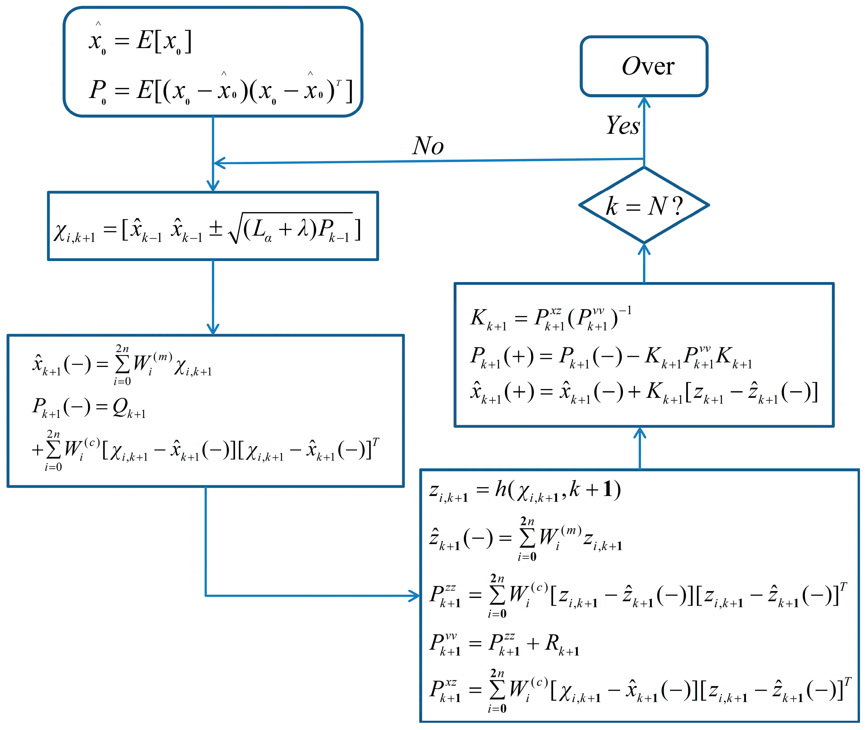
3.2. The TRPFC of Longitudinal and Lateral Force Estimation Algorithm Based on UKF

The slip ratio is as follows:
s x = ω r cos α v w v w   b r a k i n g ω r cos α v w ω r cos α   d r i v i n g
s y = ω r sin α v w   b r a k i n g tan α   d r i v i n g
s R = s x 2 + s y 2 1
where α is tire slip angle; r is tire wheel radius; ω is wheel rolling angular velocity; and v w is tire longitudinal velocities.
It is mentioned in reference [51] that under six typical roads, the changing trend of the curve between the tire/road utilization friction coefficient and slip rate is similar, especially between adjacent specific roads, such as asphalt and cement or wet pebbles and snow.
The dimensionless expression of the tire model [51] can be written as follows.
F y 0 = F y 1 s y μ R max h s Re s
F x 0 = F x 1 s x μ R max h s Re s
The normalization of the tire model [51] is as follows.
F y = μ R max g F y 0
F x = μ R max g F x 0
where μ R max h , μ R max g is the TRPFC between the adjacent pavement and the target pavement and F x 0 , F y 0 are the dimensionless tire forces of lateral and longitudinal.
To estimate the TRPFC, through Equations (1)–(3) and (18)–(24), there are:
v ˙ x v y γ + m b m z ( z ˙ b θ ˙ b ) = μ f l ( F x f l 0 cos δ f m z F y f l 0 sin δ f m z ) + μ r l F x r l 0 m z + μ f r ( F x f r 0 cos δ f m z F y f r 0 sin δ f m z ) + μ r r F x r r 0 m z
v ˙ y m b m z ( z ˙ b ψ ˙ + h g ψ ¨ b ) + v x γ = + μ f r ( F y f r 0 cos δ f m z + F x f r 0 sin δ f m z ) μ r r F y r r 0 m z + μ r l F y r l 0 m z + μ f l ( F y f l 0 cos δ f m z + F x f l 0 sin δ f m z )
γ ˙ + I x z I z ψ ¨ b = μ f l ( a I z F x f l 0 sin δ f + a I z F y f l 0 cos δ f + T 2 I z F y f l 0 sin δ f T 2 I z F x f l 0 cos δ f ) μ r l ( T 2 I z F x r l 0 + b I z F y r l 0 ) + μ r r ( T 2 I z F x r r 0 b I z F y r r 0 ) + μ f r ( a I z F x f r 0 sin δ f T 2 I z F y f r 0 sin δ f + a I z F y f r 0 cos δ f + T 2 I z F x f r 0 cos δ f )
Through Equations (25)–(27), the state equation is as follows:
μ x f l ( n ) μ x f r ( n ) μ x r l ( n ) μ x r r ( n ) μ y f l ( n ) μ y f r ( n ) μ y r l ( n ) μ y r r ( n ) = I 8 × 8 μ x f l ( n 1 ) μ x f r ( n 1 ) μ x r l ( n 1 ) μ x r r ( n 1 ) μ y f l ( n 1 ) μ y f r ( n 1 ) μ y r l ( n 1 ) μ y r r ( n 1 ) + w ( t )
The equation of measurement is as follows:
O 1 = O 2 O 3 + v ( t )
O 1 = ( v ˙ x v y γ ) v y + v x γ γ ˙
O 2 = F x f l 0 cos δ f m z F x f r 0 cos δ f m z F x r l 0 m z F x r r 0 m z F y f l 0 sin δ f m z F y f r 0 sin δ f m z 0 0 F x f l 0 sin δ f m z F x f r 0 sin δ f m z 0 0 F y f l 0 cos δ f m z F y f r 0 cos δ f m z F y r l 0 m z F y r r 0 m z K ( 3 , 1 ) K ( 3 , 2 ) K ( 3 , 3 ) K ( 3 , 4 ) K ( 3 , 5 ) K ( 3 , 6 ) K ( 3 , 7 ) K ( 3 , 8 )
K ( 3 , 1 ) = a I z F x f l 0 sin δ f T 2 I z F x f l 0 cos δ f K ( 3 , 2 ) = a I z F x f r 0 sin δ f + T 2 I z F x f r 0 cos δ f K ( 3 , 3 ) = T 2 I z F x r l 0 K ( 3 , 4 ) = T 2 I z F x r r 0 K ( 3 , 5 ) = a I z F y f l 0 cos δ f + T 2 I z F y f l 0 sin δ f K ( 3 , 6 ) = a I z F y f r 0 cos δ f T 2 I z F y f r 0 sin δ f K ( 3 , 7 ) = b I z F y r l 0 K ( 3 , 8 ) = b I z F y r r 0
O 3 = μ x _ f l μ x _ f r μ x _ r l μ x _ r r μ y _ f l μ y _ f r μ y _ r l μ y _ r r T
where μ x _ i j ( i j = f l , f r , r l , r r ) means the longitudinal TRPFC between the tires and the road surface of the target pavement, respectively; μ y _ i j ( i j = f l , f r , r l , r r ) means the lateral TRPFC between the tires and the road surface of the target pavement, separately; the random variable w ( t ) means the process noise and v ( t ) means the measurement noise.
Figure 9 can be used to represent the UKF estimation process. The covariance of measurement noise is R = 0.02 I 3 × 3 ,the covariance of process noise is Q = 0.01 I 4 × 4 and the corresponding covariance matrix is set as P 0 = 0.1 I 4 × 4 .

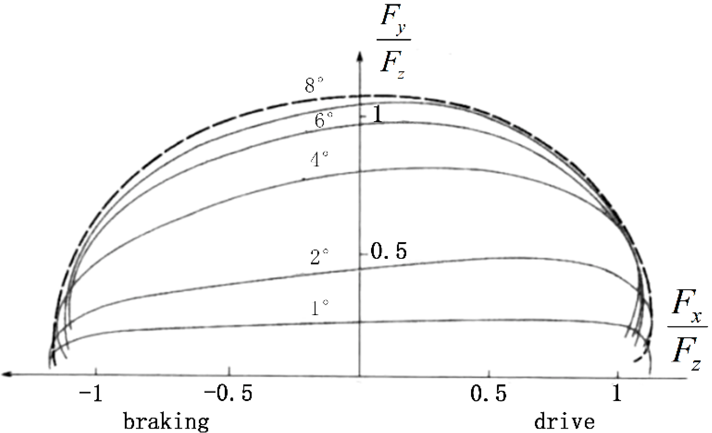
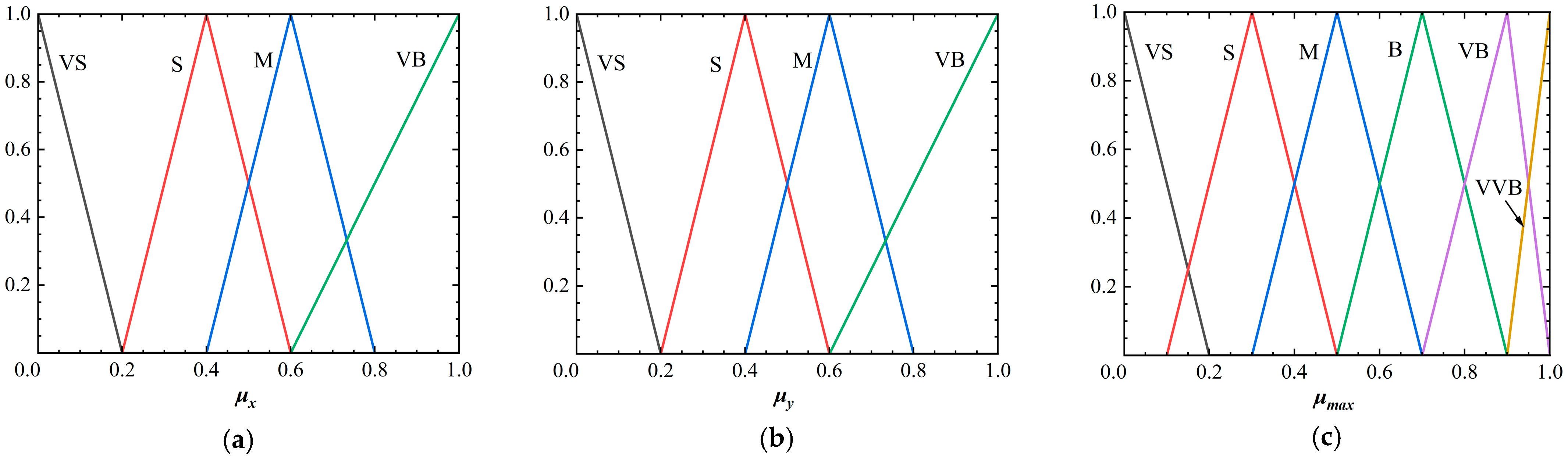
3.3. Integrated Attachment Coefficient Fusion Strategy

Figure 10 shows the “friction ellipse” effect, where the ultimate value of the longitudinal and lateral tire adhesion coefficients is less than the maximum adhesion coefficient for both lateral and longitudinal excitation. The fuzzy inference rules are formulated to fuse the lateral and longitudinal tire adhesion coefficients by using the law between the adhesion coefficients.
Step 1: Fuzzification. This step focuses on formulating the inputs and outputs’ fuzzy sets and variable theoretical domains. The theoretical domain of μ x , μ y of the input state are set to [0–1]. Using appropriate linguistic variables, the input parameters are partitioned into four fuzzy sets, and the fuzzy sets can be expressed in the form:
{ μ x } = { VS ,   S ,   M ,   VB }
{ μ y } = { VS ,   S ,   M ,   VB }
where VS, S, M, VB are very small, small, medium, and very big, respectively.
The domain of the argument of μ max for the input state is also set to [0, 1]. The suitable linguistic variables are used to divide the input parameters into six fuzzy sets, and the fuzzy sets can be defined as:
{ μ max } = { VS ,   S ,   M ,   B ,   VB ,   VVB }
where VS, S, M, B, VB, VVB are very small, small, medium, big, very big, and maximum, respectively.
Step 2: Fuzzy decision process. The rule of fuzzy is the most critical part of the whole method and has a crucial influence on the output. In this step, the coupling relationship between the attachment coefficients is used to develop fuzzy inference rules. Table 2 shows the fuzzy rules.
Step 3: Defuzzification. Under the given input condition, the fuzzy set of output states can be obtained using the Mamdani method [52] through the fuzzy rules shown in Table 2. To transform fuzzy values into clear values, the centroid method is used to de-blur. Figure 11 shows the slip rate membership function.
Step 4: Optimize the membership function. The membership function corresponding to each parameter is optimized through experiments.
The fuzzy method fuses the pavement adhesion coefficients of lateral and longitudinal based on the coupling process of lateral and longitudinal forces and the friction ellipse effect. This method can accurately obtain the TRPFC, and the fusion results are shown in Section 4.

4. Simulation Test

In this paper, Carsim and Matlab/Simulink are used to simulate the linear braking condition and curve braking condition of wet pebbles and snow pavement.

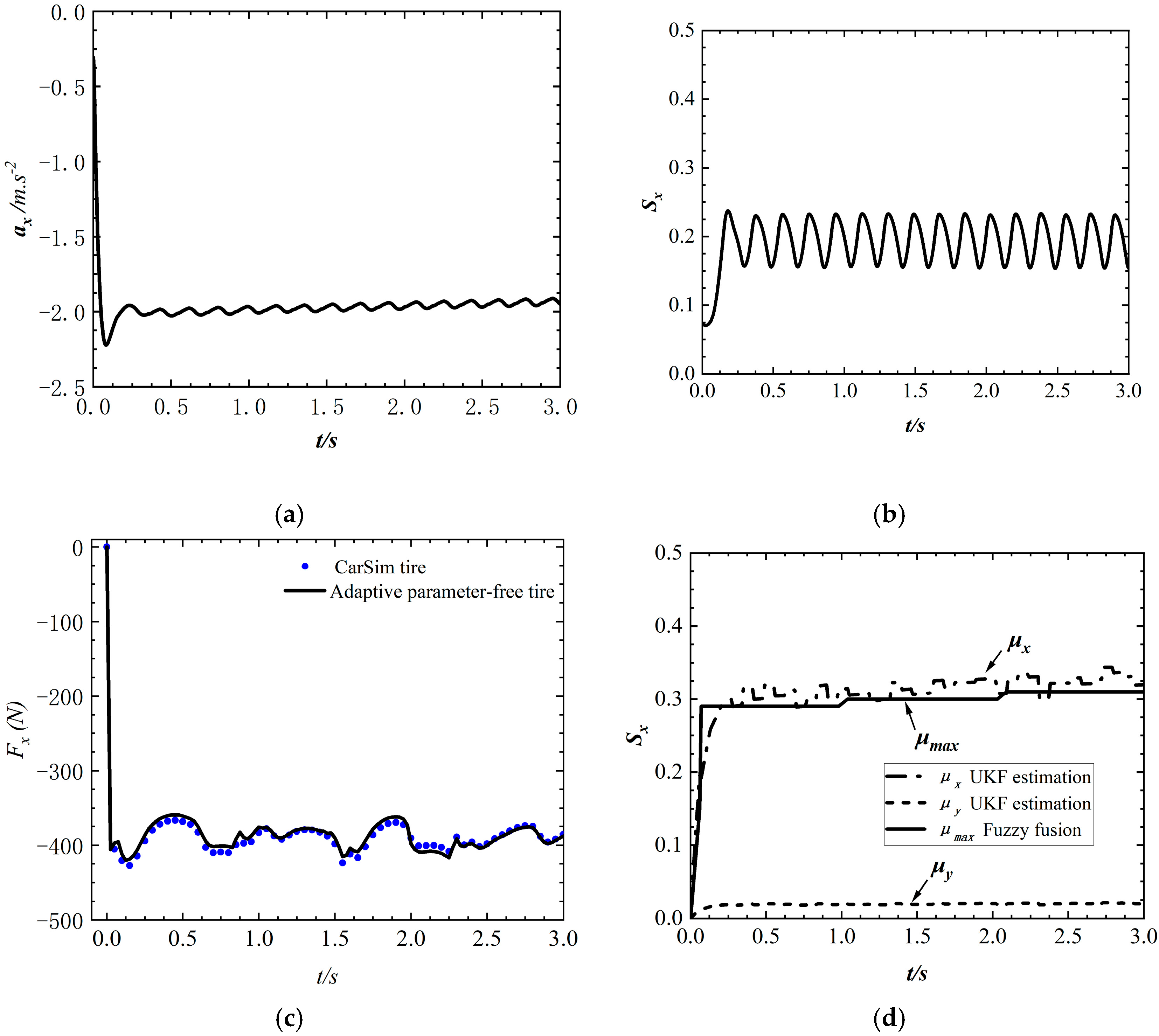
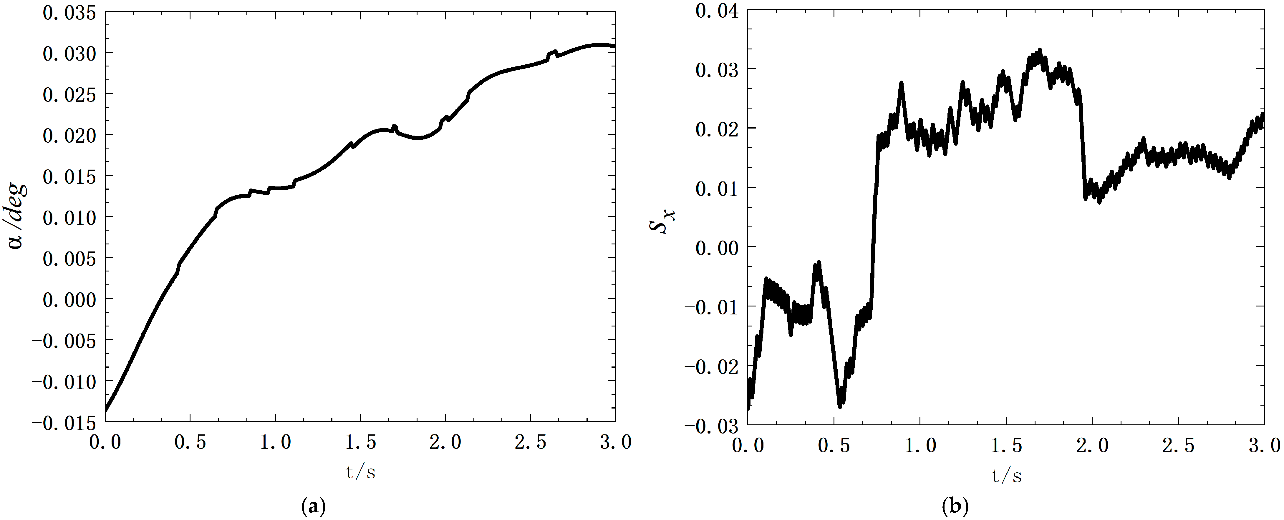
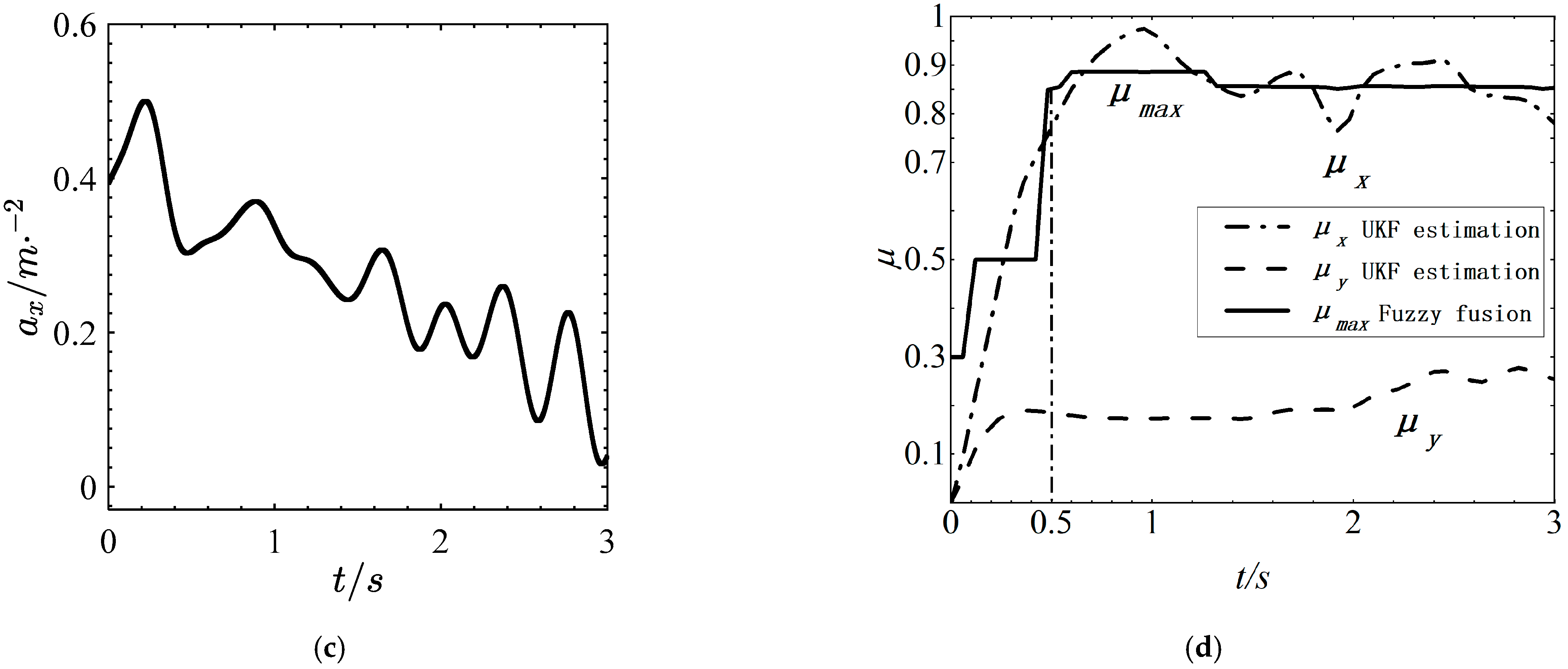
4.1. Straight Line Test
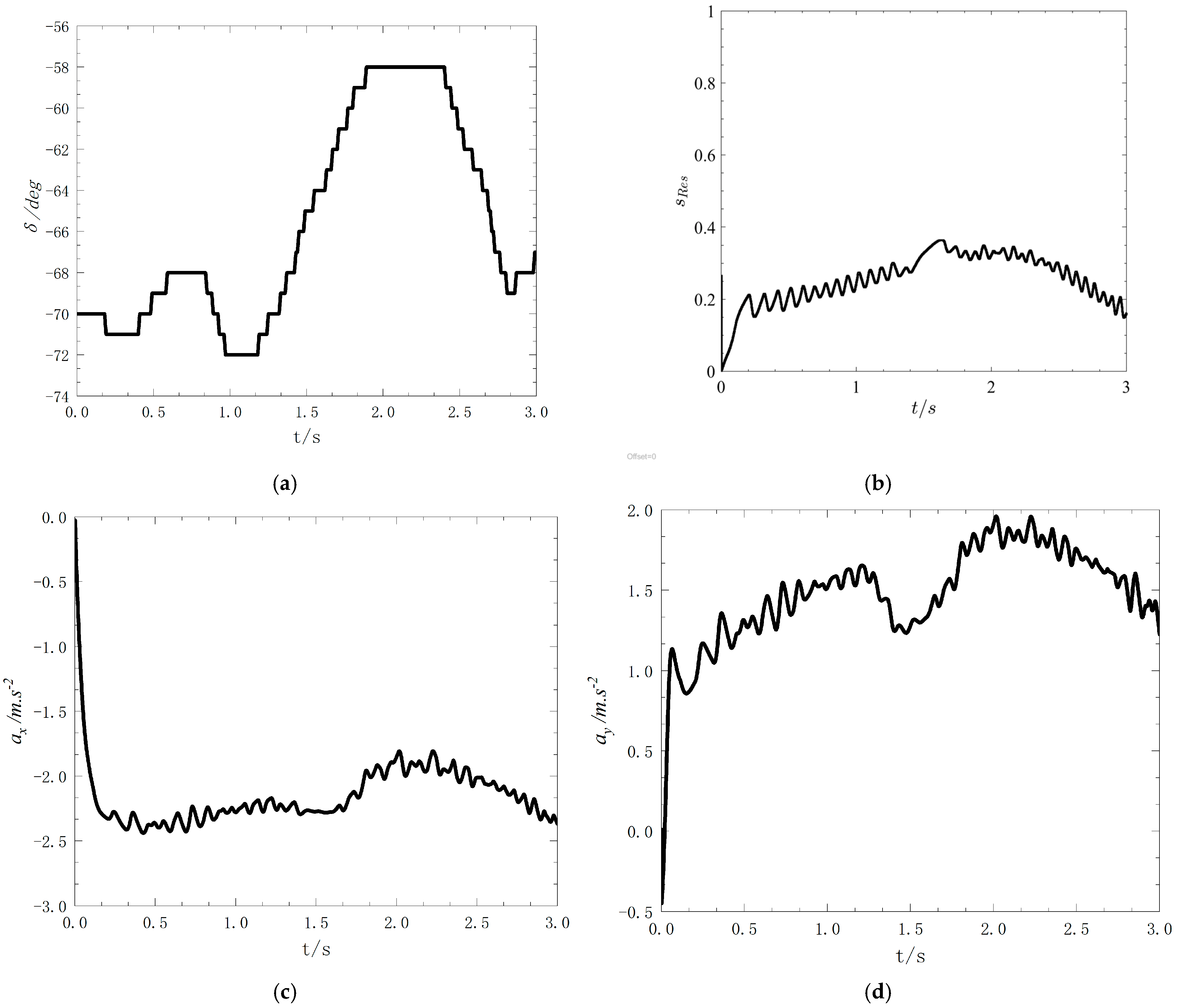
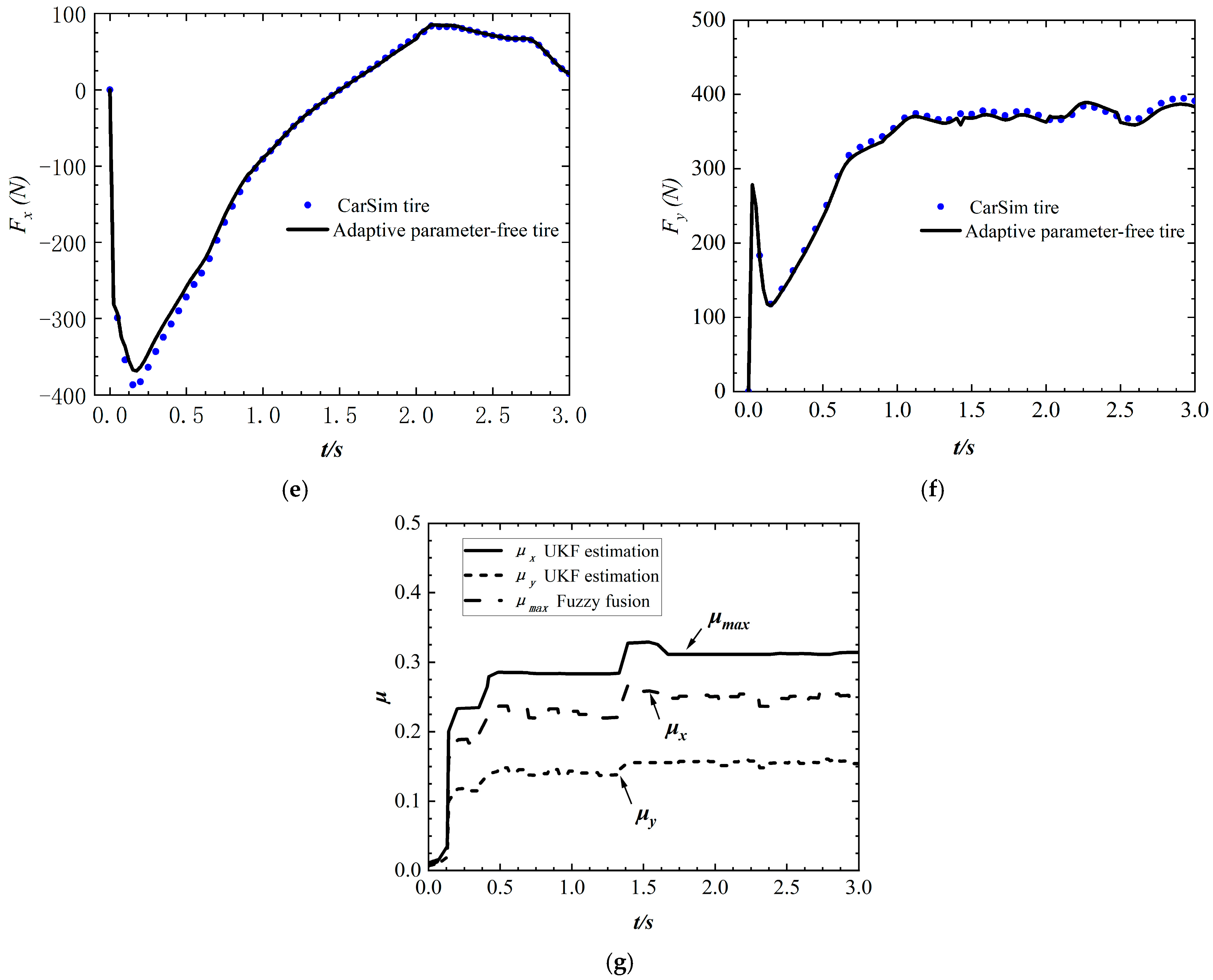
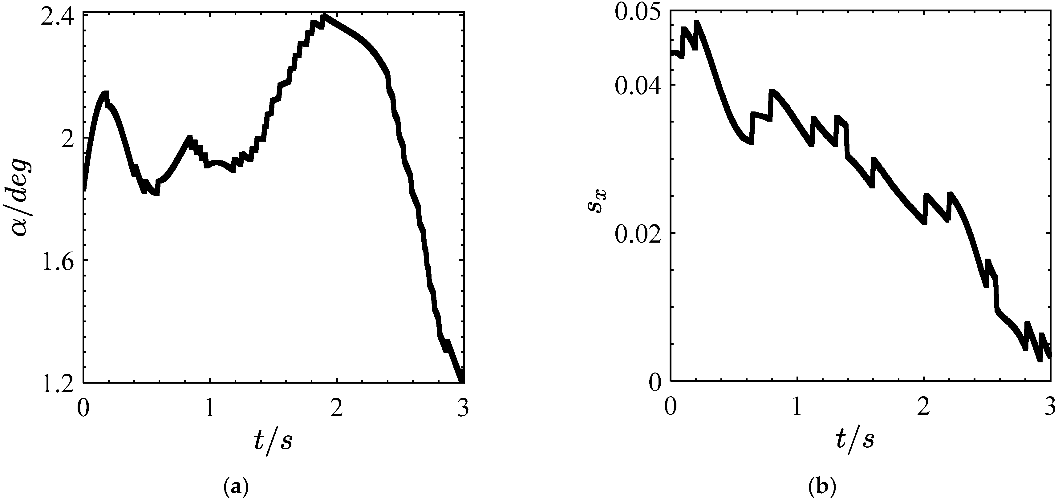
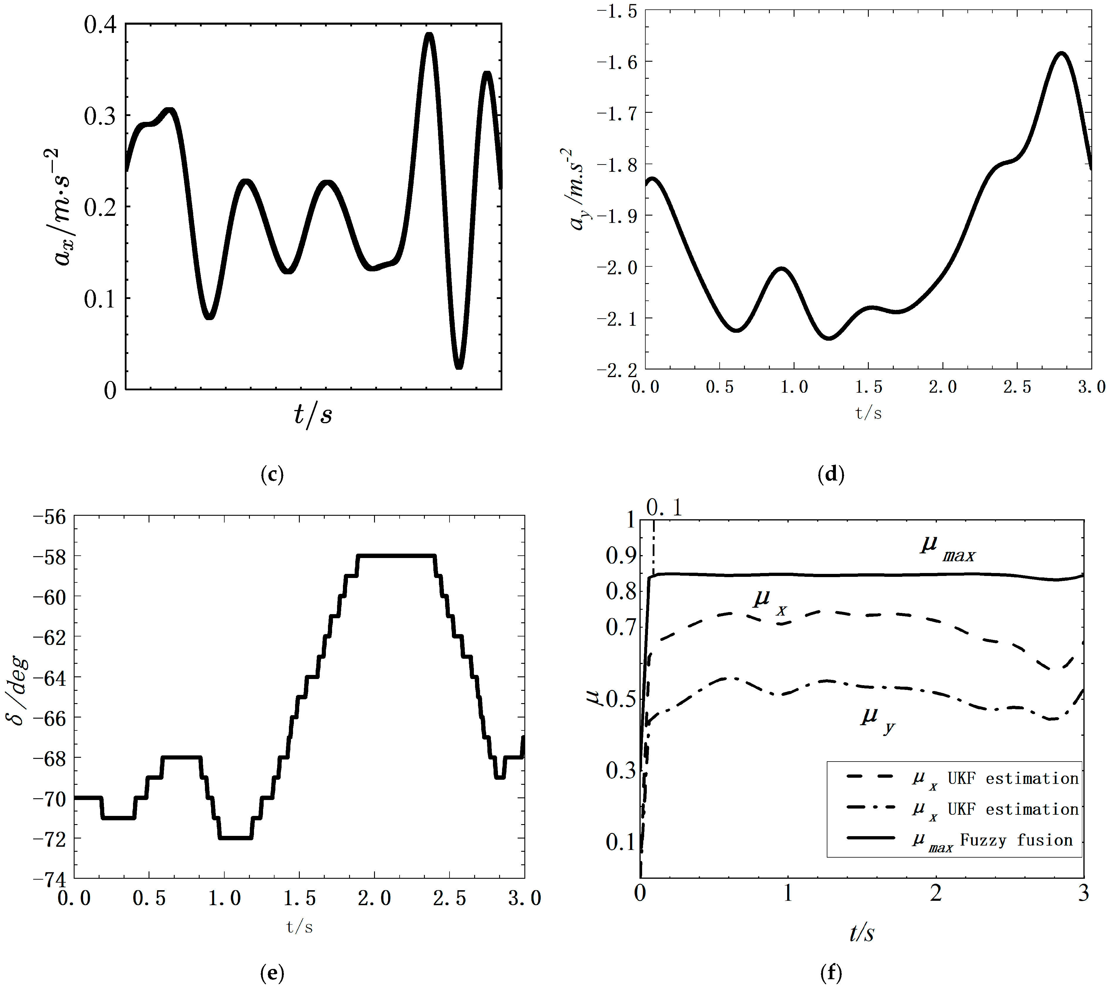
In order to simulate the wet cobblestone and snow pavement, the road adhesion coefficient is set to 0.3, and the initial speed of the vehicle is 60 km/h, and the straight-line braking test is carried out. The simulation results are shown in Figure 12a–c.
Because the adhesion coefficients of the four wheels on the road surface are the same, the left front wheel is taken as an example for simulation.
It can be seen from Figure 12a–d that the slip rate is stable at 0.2 because the vehicle has started the ABS function so that the slip rate is steady in the optimal range. The maximum longitudinal acceleration of the vehicle reaches 2.25 m/s2. The trend of longitudinal force is consistent as a whole, and RRMSE value is less than 0.1028. When the maximum adhesion coefficient is within 0.15 s, it converges to 0.3, and then the estimation error is stable within [0, 0.02].

4.2. Curved Test

In order to simulate the wet cobblestone and snow pavement, the road adhesion coefficient is set to 0.3, the road is set as a circular road with a radius of 33 m, and the initial speed of the vehicle is 60 km/h. The curve deceleration condition is set. The simulation results are shown in Figure 13a–e.
Because the adhesion coefficients of the four wheels on the road surface are the same, the left front wheel is taken as an example for simulation.
It can be seen from Figure 13a–g that the slip ratio is stable between 0.2 and 0.4. The maximum longitudinal acceleration of the vehicle is 2.5 m/s2, and the maximum lateral acceleration is 2 m/s2. The trends of longitudinal force and lateral force are generally consistent, and the RRMSE values are less than 0.1048 and 0.1102, respectively. When the maximum adhesion coefficient is within 0.5 s, it converges to 0.3, and then the estimation error is stable within [−0.03, 0.04].

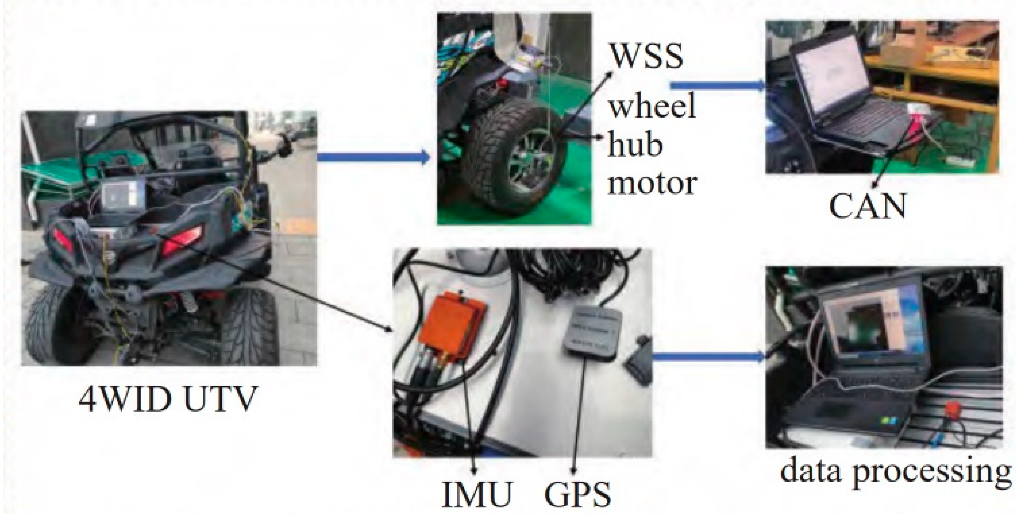
5. Real Vehicle Test

The test platform is a four-wheel independently driven vehicle modified by wire (UTV). The WSS sensor embedded in the hub motor can measure the four wheels’ rotation speed and angle. The signal is fed to the computer via the CAN bus. The IMU model of vehicle inertial navigation is MTI-G-710, and the sampling period is 2.5 ms. Figure 14 shows the experimental vehicle, sensors, and data acquisition hardware.

5.1. Straight Line Test

On the dry asphalt road, the straight driving condition is fixed. The peak coefficient of friction is within the limit of [0.8, 0.91] [51], which is based on the data available. The average speed of the vehicle is kept at 60 km/h. Using the left front wheel as the demonstration result, Figure 15 shows the test results.
AS Figure 15d shows, the TRPFC converges to 0.83 prior to 0.5s and then fluctuates around 0.85 under the straight braking condition; however, the overall error is stable to within ±0.05. The longitudinal slip velocity in Figure 15b has a negative value because of the incomplete synchronization of the four-wheel speed of the electric vehicle as well as the fluctuation error of inertial navigation. However, it does not have any effect on the result.

5.2. Curved Test

On the dry asphalt road, the curved driving condition is fixed. The average speed of the vehicle is kept at 60 km/h. The radius is 33 m. Using the left front wheel as the demonstration result, Figure 16 shows the test results.
As shown in Figure 16f, the TRPFC converges to 0.85 in less than 0.1 s and then fluctuates around 0.85, but the overall error is stable to within ± 0.02.
According to the experimental analysis, when braking in a straight line, the longitudinal adhesion coefficient of the vehicle is significant, but the lateral adhesion coefficient is small. At this time, the fused estimated value keeps an approximate relationship with the numerical range of the longitudinal adhesion coefficient. During cornering braking, when both longitudinal and lateral road excitation is extensive, both longitudinal and lateral tire utilization adhesion coefficients play an essential role in the contact process between the three-dimensional road surface and the tire. At this time, the fuzzy fusion method can still accurately estimate the TRPFC of the actual road surface.

6. Conclusions

To estimate the TRPFC accurately, a new method of three-dimensional pavement fusion adhesion coefficient based on a dimensionless data-driven tire model is proposed. The stress distribution law and multi-point contact model between tire and road are introduced to represent three-dimensional pavement excitation accurately. A new dimensionless data-driven tire model is proposed to describe the tire/road contact state during driving. A fuzzy reasoning strategy is designed to fuse the longitudinal and lateral adhesion coefficients obtained by the UKF algorithm, and finally, the accurate peak adhesion coefficient of pavement is estimated.
Based on the results on real vehicles, we can come to the conclusion that this algorithm can estimate the peak adhesion coefficient within 0.5 s, and the error is maintained within ±0.05, demonstrating that the algorithm can estimate the TRPFC accurately and promptly. The vehicle’s sensors can directly obtain the parameters needed in this paper, and the identification results help estimate the safe distance and braking force, which is particularly valuable for improving active vehicle safety and reducing the occurrence of road traffic accidents.
In the next step, we will verify the algorithm in this paper on a variety of roads, especially on low-adhesion roads, and in order to expand the application scope of the algorithm in this paper, we will migrate the algorithm to the truck for verification.

Author Contributions

Conceptualization, Y.L.; formal analysis, Y.L.; funding acquisition, Y.L.; investigation, Z.X., N.C. and Y.H.; methodology, Z.X. and Y.L.; resources, Y.L.; software, Z.X.; supervision, Y.L.; validation, Z.X., Y.L. and Y.H.; writing—original draft, Z.X.; writing—review and editing, Z.X., Y.L. and Y.H. All authors have read and agreed to the published version of the manuscript.

Funding

This work was supported by the National Natural Science Foundation of China under grant number 12072204; National Natural Science Foundation of China under grant number 11572207; Natural Science Foundation of Hebei Province under grant number A2020210039.

Institutional Review Board Statement

Not applicable.

Informed Consent Statement

Not applicable.

Data Availability Statement

Not applicable.

Conflicts of Interest

The authors declare no conflict of interest.

References

  1. National Data Traffic Accident Statistics. China National Bureau of Statistics. 2021. Available online: https://data.stats.gov.cn/easyquery.htm?cn=C01&zb=A0S0D01&sj=2021 (accessed on 5 June 2020).
  2. World Health Organization. Global Status Report on Road Safety 2015; World Health Organization: Geneva, Switzerland, 2015. [Google Scholar]
  3. Xianjian, J.; Jiadong, W.; Zeyuan, Y.; Liwei, X.; Guodong, Y.; Nan, C. Robust Vibration Control for Active Suspension System of In-Wheel-Motor-Driven Electric Vehicle Via mu-Synthesis Methodology. ASME Trans. J. Dyn. Syst. Meas. 2022, 144, 051007. [Google Scholar]
  4. Wang, F.; Lu, Y.; Li, H. Heavy-duty vehicle braking stability control and hil verification for improving traffic safety. J. Adv. Transp. 2022, 2022, 5680599. [Google Scholar] [CrossRef]
  5. Lu, Y.; Wang, T.; Zhang, H. Multiobjective Synchronous Control of Heavy-Duty Vehicles Based on Longitudinal and Lateral Coupling Dynamics. Shock. Vib. 2022, 2022, 6987474. [Google Scholar] [CrossRef]
  6. Khaleghian, S.; Emami, A.; Taheri, S. A technical survey on tire-road friction estimation. Friction 2017, 5, 123–146. [Google Scholar] [CrossRef] [Green Version]
  7. Alonso, J.; López, J.M.; Pavón, I.; Recuero, M.; Asensio, C.; Arcas, G.; Bravo, A. On-board wet road surface identification using tyre/road noise and support vector machines. Appl. Acoust. 2014, 76, 407–415. [Google Scholar] [CrossRef]
  8. Xiong, Y.; Yang, X. A review on in-tire sensor systems for tire-road interaction studies. Sens. Rev. 2018, 38, 231–238. [Google Scholar] [CrossRef]
  9. Gao, L.; Xiong, L.; Lin, X.; Xia, X.; Liu, W.; Lu, Y.; Yu, Z. Multi-sensor fusion road friction coefficient estimation during steering with Lyapunov method. Sensors 2019, 19, 3816. [Google Scholar] [CrossRef] [Green Version]
  10. Leng, B.; Jin, D.; Xiong, L.; Yang, X. Estimation of tire-road peak friction coefficient for intelligent electric vehicles based on camera and tire dynamics information fusion. Mech. Syst. Signal Process. 2021, 150, 107275. [Google Scholar] [CrossRef]
  11. Wang, Y.; Liang, G.; Wei, Y. Road Identification Algorithm of Intelligent Tire Based on Support Vector Machine. J. Automot. Eng. 2020, 42, 1671–1678+1717. [Google Scholar]
  12. Erdogan, G.; Alexander, L.; Rajamani, R. Estimation of tire road friction coefficient using a novel wireless piezoelectric tire sensor. IEEE Sens. J. 2011, 11, 267–279. [Google Scholar] [CrossRef]
  13. Khaleghian, S. The Application of Intelligent Tires and Model-Based Estimation Algorithms in Tire-Road Contact Characterization; Virginia Polytechnic Institute and State University: Blacksburg, VA, USA, 2017. [Google Scholar]
  14. Niskanen, A.J.; Tuononen, A.J. Three 3-axis accelerometers fixed inside the tire for studying contact patch deformations in wet conditions. Veh. Syst. Dyn. 2014, 52 (Supp. S1), 287–298. [Google Scholar] [CrossRef]
  15. Niskanen, A.J.; Tuononen, A.J. Accelerometer tire to estimate the aquaplaning state of the tire-road contact. Intell. Veh. Symp. (IV) 2015, 2015, 343–348. [Google Scholar]
  16. Alexander, L.; Rajamani, R. Tire road friction coefficient estimation. J. Dyn. Syst. Meas. Control 2004, 126, 265–275. [Google Scholar]
  17. Chen, G.; Wang, X.; Su, L.; Wang, Y. Safety distance model for longitudinal collision avoidance of logistics vehicles considering slope and road adhesion coefficient. Proc. Inst. Mech. Eng. J. Automob. Eng. 2020, 235, 498–512. [Google Scholar]
  18. Li, G.; Zong, C.F.; Zhang, Q.; Hong, W. Acceleration slip regulation control of 4 WID electric vehicles based on fuzzy road identification. J. South China Univ. Technol. 2012, 40, 99–104. [Google Scholar]
  19. Zhang, X.; Gohlich, D. A hierarchical estimator development for estimation of tire-road friction coefficient. PLoS ONE 2017, 12, e0171085. [Google Scholar] [CrossRef] [Green Version]
  20. Yang, X.; Li, J.; Zhang, K. Study on vehicle adaptive cruise control based on road surface adhesion coefficient estimation. J. Nanjing Univ. Sci. Technol. 2018, 42, 466–473. [Google Scholar]
  21. Xin, X.; Lu, X.; Kai, S.; Yu, Z.P. Estimation of maximum road friction coefficient based on Lyapunov method. Int. J. Automot. Technol. 2016, 17, 991–1002. [Google Scholar]
  22. Lin, F.; Huang, C. Using UKF algorithm to estimate road surface adhesion coefficient. J. Harbin Inst. Technol. 2013, 45, 115–120. [Google Scholar]
  23. Siramdasu, Y.; Li, K.; Wheeler, R. Virtual Generation of Flexible Ring Tire Models Using Finite Element Analysis: Application to Dynamic Cleat Simulations. Tire Sci. Technol. 2022, 50, 288–315. [Google Scholar] [CrossRef]
  24. Polasik, J.; Waluś, K.J.; Warguła, Ł. Experimental studies of the size contact area of a summer tire as a function of pressure and the load. Procedia Eng. 2017, 177, 347–351. [Google Scholar] [CrossRef]
  25. He, H.; Li, R.; Yang, Q.; Pei, J.; Guo, F. Analysis of the tire-pavement contact stress characteristics during vehicle maneuvering. KSCE J. Civ. Eng. 2021, 25, 2451–2463. [Google Scholar] [CrossRef]
  26. Xiong, Y.; Tuononen, A. Rolling deformation of truck tires: Measurement and analysis using a tire sensing approach. J. Terramechanics 2015, 61, 33–42. [Google Scholar] [CrossRef]
  27. Wach, W.; Zębala, J. Striated Tire Yaw Marks—Modeling and Validation. Energies 2021, 14, 4309. [Google Scholar] [CrossRef]
  28. Dudziak, M.; Lewandowski, A.; Waluś, K.J. Static tests the stiffness of car tires. IOP Conf. Ser. Mater. Sci. Eng. 2020, 776, 012071. [Google Scholar] [CrossRef]
  29. KuliKowsKi, K.; Szpica, D. Determination of directional stiffnesses of vehicles’ tires under a static load operation. Eksploat. I Niezawodn. 2014, 16, 66–72. [Google Scholar]
  30. Liang, G.; Wang, Y.; Garcia, M.A.; Zhao, T.; Liu, Z.; Kaliske, M.; Wei, Y. A Universal Approach to Tire Forces Estimation by Accelerometer-Based Intelligent Tire: Analytical Model and Experimental Validation. Tire Sci. Technol. 2022, 50, 2–26. [Google Scholar] [CrossRef]
  31. Dong, X.; Tao, S.; Zhang, H. Robust Lateral and Longitudinal Tire Force Estimation Based on PMI Observer for Intelligent Vehicle. In Proceedings of the 2022 IEEE 5th International Conference on Industrial Cyber-Physical Systems (ICPS), Coventry, UK, 24–26 May 2022; pp. 1–6. [Google Scholar]
  32. Zhu, J.J.; Khajepour, A.; Spike, J.; Chen, S.K.; Moshchuk, N. An integrated vehicle velocity and tyre-road friction estimation based on a half-car model. Int. J. Veh. Auton. Syst. 2016, 13, 114–139. [Google Scholar] [CrossRef]
  33. Liu, X.; Cao, Q.; Wang, H.; Chen, J.; Huang, X. Evaluation of vehicle braking performance on wet pavement surface using an integrated tire-vehicle modeling approach. Transp. Res. Rec. 2019, 2673, 295–307. [Google Scholar] [CrossRef]
  34. Saha, A.; Wahi, P.; Wiercigroch, M.; Stefański, A. A modified LuGre friction model for an accurate prediction of friction force in the pure sliding regime. Int. J. Non-Linear Mech. 2016, 2019, 122–131. [Google Scholar] [CrossRef]
  35. Gim, G.; Nikravesh, P.E. An analytical model of pneumatic tires for vehicle dynamic simulations. Part 1: PureSlips. Int. J. Veh. Des. 1990, 11, 589–618. [Google Scholar]
  36. Gim, G.; Nikravesh, P.E. A three-dimensional tire model for steady-state simulations of vehicles. SAE Trans. 1993, 102, 150–159. [Google Scholar]
  37. Dugoff, H.; Fancher, P.S.; Sege, L. An analysis of tire traction properties and their influence on vehicle dynamic performance. SAE Trans. 1970, 1219–1243. [Google Scholar]
  38. Hahn, J.; Rajamani, R.; Alexander, L. GPS-based real-time identification of tire-road friction coefficient. Ransactions Control. Syst. Technol. 2002, 10, 331–343. [Google Scholar] [CrossRef]
  39. De Wit, C.; Olsson, H.; Astroem, K.J.; Lischinsky, P. A new model for control of systems with friction. Trans. Autom. Control. 1995, 40, 419–425. [Google Scholar] [CrossRef] [Green Version]
  40. Burckhardt, M. Wheel Slip Control Systems; Vogel Verlag: Würzburg, Germany, 1993. [Google Scholar]
  41. Zhang, X.; Wang, F.; Wang, Z.; Li, W.; He, D. Intelligent tires based on wireless passive surface acoustic wave sensors. In Proceedings of the 7th International IEEE Conference on Intelligent Transportation Systems (IEEE Cat. No. 04TH8749), Washington, WA, USA, 3–6 October 2004; Volume 2004, pp. 960–964. [Google Scholar]
  42. Kuiper, E.; Van Oosten, J.M. The PAC2002 advanced handling tire model. Veh. Syst. Dyn. 2007, 45, 153–167. [Google Scholar] [CrossRef]
  43. Bakker, E.; Nyborg, L.; Pacejka, H.B. Tire modeling for use in vehicle dynamics studies. SAE Int. Congr. Expo. 1987, 190–204. [Google Scholar]
  44. Song, Y.; Shu, H.; Chen, X.; Luo, S. Direct-yaw-moment control of four-wheel-drive electrical vehicle based on lateral tire–road forces and tire slip angle observer. IET Intell. Transp. Syst. 2019, 13, 303–312. [Google Scholar] [CrossRef]
  45. Guo, K. UniTire: Unified Tire Model. J. Mech. Eng. 2016, 52, 90–99. [Google Scholar] [CrossRef]
  46. Rajamani, R. Vehicle Dynamics and Control, 2nd ed.; Springer Science: London, UK, 2012. [Google Scholar]
  47. Han, Y.; Lu, Y.; Liu, J.; Zhang, J. Research on Tire/Road Peak Friction Coefficient Estimation Considering Effective Contact Characteristics between Tire and Three-Dimensional Road Surface. Machines 2022, 10, 614. [Google Scholar] [CrossRef]
  48. Lu, Y.; Zhang, J.; Li, H.; Ma, Z. Research on tire-road system coupling dynamics based on non-uniform contact. J. Mech. Eng. 2021, 57, 87–98. [Google Scholar]
  49. Lu, Y.; Zhang, J.; Yang, S.; Yang, S.; Li, Z. Study on improvement of LuGre dynamical model and its application in vehicle handling dynamics. J. Mech. Sci. Technol. 2019, 33, 545–558. [Google Scholar] [CrossRef]
  50. Lu, Y.; Zhang, J.; Yang, S.; Li, Z. Construction of Three-Dimensional Road Surface and Application on Interaction between Vehicle and Road. Shock. Vib. 2018, 2018, 1–14. [Google Scholar]
  51. Han, Y.; Lu, Y.; Chen, N.; Wang, H. Research on the Identification of Tire Road Peak Friction Coefficient under Full Slip Rate Range Based on Normalized Tire Model. Actuators 2022, 11, 59. [Google Scholar] [CrossRef]
  52. Tahami, F.; Farhangi, S.; Kazemi, R. A fuzzy logic direct yaw-moment control system for all-wheel-drive electric vehicles. Veh. Syst. Dyn. 2004, 41, 203–221. [Google Scholar] [CrossRef]
Figure 1. Vehicle planar four-wheel dynamics models.
Machines 11 00189 g001
Figure 2. Experiment of tire and vertical load. (a) Experimental operation. (b) Contact length curve fitting. (c) Contact area curve fitting.
Machines 11 00189 g002aMachines 11 00189 g002b
Figure 3. Tire contact stress distribution diagram.
Machines 11 00189 g003
Figure 4. Tire and three-dimensional road vertical dynamic contact models.
Machines 11 00189 g004
Figure 5. Adaptive parameter-free tire model based on data driven model.
Machines 11 00189 g005
Figure 6. Longitudinal force contrast curve. (a) μ = 0.9 . (b) μ = 0.3 .
Machines 11 00189 g006
Figure 7. Lateral force contrast curve. (a) μ = 0.9 . (b) μ = 0.3 .
Machines 11 00189 g007
Figure 9. UKF estimation process.
Machines 11 00189 g009
Figure 10. Distribution of longitudinal and lateral adhesion coefficient limits (friction ellipse).
Machines 11 00189 g010
Figure 11. Affiliation function for peak pavement adhesion coefficient. (a) Affiliation function for the longitudinal attachment coefficient. (b) Affiliation function for lateral attachment coefficient. (c) Pavement peak adhesion coefficient affiliation function.
Machines 11 00189 g011
Figure 12. Simulation results under linear braking conditions. (a) Longitudinal acceleration. (b) Longitudinal slip rate. (c) Longitudinal force contrast curve. (d) Estimated results of pavement adhesion coefficient.
Machines 11 00189 g012
Figure 13. Simulation results under combined bending braking conditions. (a) Steering wheel cornering. (b) Longitudinal slip rate. (c) Longitudinal acceleration. (d) Lateral acceleration. (e) Longitudinal force contrast curve. (f) Lateral force contrast curve. (g) Estimated pavement adhesion coefficient.
Machines 11 00189 g013aMachines 11 00189 g013b
Figure 14. Experimental vehicle and sensor equipment.
Machines 11 00189 g014
Figure 15. Simulation results under linear braking conditions. (a) Lateral deflection angle. (b) Longitudinal slip rate. (c) Longitudinal acceleration. (d) Estimated results of pavement adhesion coefficient.
Machines 11 00189 g015aMachines 11 00189 g015b
Figure 16. Simulation results under combined bending braking conditions. (a) Lateral deflection angle. (b) Longitudinal slip rate. (c) Longitudinal acceleration. (d) Lateral acceleration. (e) Steering wheel cornering. (f) Estimated pavement adhesion coefficient.
Machines 11 00189 g016aMachines 11 00189 g016b
Table 1. Key parameters of the vehicle.
SymbolValueName of Parameter
m z 880 kgTotal vehicle mass
m b 788 kgSprung mass
L2.040 mWheel base
a1.145 m Distance from front axle to centroid
b0.895 mDistance from rear axle to centroid
h g 0.54 m Centroid height
T1.3 m Width of wheel track
I z 832.3 kg·m2Moment of inertia about the z-axis
Kψ25,041 N/radTire cornering stiffness
K b 19.6 Kn/mStiffness coefficient of suspension system
c b 1450 N·s/m2Damping constant of suspension buffer
K w 250 Kn/mStiffness coefficient of tire
C w 3375 N·s/m2Damping coefficient of tire
Table 2. Fuzzy inference rules.
Lateral SlipLongitudinal Slip
VSSMVB
VSVSSM VB
SMMBVB
MBBBVB
VBVBVBVBVVB
Disclaimer/Publisher’s Note: The statements, opinions and data contained in all publications are solely those of the individual author(s) and contributor(s) and not of MDPI and/or the editor(s). MDPI and/or the editor(s) disclaim responsibility for any injury to people or property resulting from any ideas, methods, instructions or products referred to in the content.

