Article

Fingerprinting-Based Indoor Positioning Using Data Fusion of Different Radiocommunication-Based Technologies

1
Department of Mechatronics and Automation, Faculty of Engineering, University of Szeged, Moszkvai krt. 9, 6725 Szeged, Hungary
2
Doctoral School of Applied Informatics and Applied Mathematics, Óbuda University, Bécsi str. 96/b, 1034 Budapest, Hungary
*
Author to whom correspondence should be addressed.
Machines 2023, 11(2), 302; https://doi.org/10.3390/machines11020302
Submission received: 23 January 2023 / Revised: 12 February 2023 / Accepted: 16 February 2023 / Published: 17 February 2023
(This article belongs to the Special Issue Modeling, Sensor Fusion and Control Techniques in Applied Robotics)

Abstract

:
Wireless-radio-communication-based devices are used in more and more places with the spread of Industry 4.0. Localization plays a crucial part in many of these applications. In this paper, a novel radiocommunication-based indoor positioning method is proposed, which applies the fusion of fingerprints extracted with various technologies to improve the overall efficiency. The aim of the research is to apply the differences, which occur due to that different technologies behave differently in an indoor space. The proposed method was validated using training and test data collected in a laboratory. Four different technologies, namely WiFi received signal strength indication (RSSI), ultra-wideband (UWB) RSSI, UWB time of flight (TOF) and RSSI in 433 MHz frequency band and all of their possible combinations, were tested to examine the performance of the proposed method. Three widely used fingerprinting algorithms, the weighted k-nearest neighbor, the random forest, and the artificial neural network were implemented to evaluate their efficiency with the proposed method. The achieved results show that the accuracy of the localization can be improved by combining different technologies. The combination of the two low-cost technologies, i.e., the WiFi and the 433 MHz technology, resulted in an 11% improvement compared to the more accurate technology, i.e., the 433 MHz technology. Combining the UWB module with other technologies results in a less significant improvement since this sensor provides lower error rates, when used alone.

1. Introduction

With the spread of Industry 4.0, various wireless communication technologies play an increasingly important role in many areas [1]. The Internet of Things (IoT) has great potential for use in public transport, home automation, healthcare, agriculture, and even industrial applications [1,2,3]. These smart things, smart devices, maintain the connection between the user and the several sensors and actuators. In most cases, these modules can be organized into a network so they can form a wireless sensor network (WSN) [2,3,4,5,6]. These WSNs are made up of nodes that are connected to each other and communicate with each other to exchange or transmit information. They also provide information for the user. The node must be configured so that its energy consumption should be as low as possible. It usually contains at least one sensor, and possibly some kind of actuator, if intervention is also required. A node is controlled by a processing unit, which is usually a microcontroller. In addition, it is also necessary to use a communication interface to transmit data within the network. This is usually a transceiver, so transmitter and receiver at the same time, and it can communicate in both directions: sending and receiving data packets [6].
The IoT’s main features include [1]:
  • Wide range: the range of IoT devices is extremely wide, there are a lot of communication standards that can be used for creating the network;
  • Intelligence: by integrating software algorithms and appropriate hardware devices, IoT devices become “smart”, communicate with each other and with the user;
  • Sensing: sensors are needed to monitor the environment, changes in the environment, and to be able to intervene;
  • Complex systems: it is possible to create systems with a complex structure both in terms of hardware and software;
  • A lot of data: since many devices are used in IoT systems, a lot of data is generated by them;
  • Low power consumption: most devices are designed so that they do not consume much energy.
Some of their most important fields of application are localization and positioning [4,5,6,7,8,9,10,11], during which the position and the change of the position of people, robots, and other devices need to be determined as precisely as possible. The number of available radiocommunication-based technologies and localization methods have increased significantly due to the spread of Industry 4.0 [11].
The most important localization system is GPS, which cannot be used indoors, due to the line of sight (LOS) requirements between the device and the satellites. Because of the external walls, this is not feasible in buildings, so in such cases it is extremely inaccurate. It is possible to use this technology indoors by installing indoor GPS transceivers, which are expensive, consume a lot of energy, and it is complicated to expand the system, while it also has a large error compared to other technologies [11]. On the other hand, the most important requirements for localization systems are that they are cheap, low-power and are easily expandable [4,5].
Indoor positioning systems (IPS) can be grouped based on several criteria. According to the type of technology, there are technologies using electromagnetic waves, e.g., ultra-wideband (UWB) [12,13,14,15], Bluetooth low energy (BLE) [16,17,18,19], radio frequency identification (RFID) [20,21], WiFi [22,23,24,25,26], ZigBee [27,28], magnetic [29,30], sound-based [31,32], and optical [33] methods such as camera [34], light detection and ranging (LiDar) [35], infrared (IR) or visible light communications (VLC) technologies. In addition, the position estimation methods using radiocommunication-based technologies can be divided into two large groups [8,36]. One includes range-based methods, when the distance between the receiver and the transceiver modules should be determined. For this purpose, the received signal strength indicator (RSSI) [16] is widely used. After the measurement of the RSSI between two units, the distance can be calculated with the help of the free space path loss (FSPL) model. In the group of range-based methods other techniques also exist, which use time or geometric measurement to determine the distance. These methods can be based on various extracted parameters, such as the time of arrival (TOA) [27], angle of arrival (AOA) [37], time difference of arrival (TDOA) [38] and round-trip time of flight (RTOF) [17] measurements. There are absolute methods for calculating the position, such as trilateration, multilateration, triangulation, fingerprinting, proximity-based and image-processing-based methods. Relative methods can be found as well, such as the dead reckoning. The other method contains the range-free methods, including pattern matching/fingerprinting and hop-count-based methods. The fingerprinting method has two phases. Firstly, a database needs to be created. Creating the database is the specific offline stage when the measurement is taken at specific points in a room to create a radio map. The number of maps depends on the number of anchors, i.e., the number of nodes with fixed coordinates. The map is mostly based on an RSSI measurement. After the radio map is created, the online stage follows. The online stage is the active localization stage. In this case, the actual position of the device can be determined. The applicability of range-based methods is determined by the capabilities of the modules/nodes because these methods can only be used if the desired position is within the range of the reference nodes or anchors. These methods require often additional hardware (i.e., AOA). When performing time measurement with TOA, clock synchronization must be performed, which affects the performance of the localization. The biggest advantage of range-free methods is that they are easier to use, but the localization accuracy is worse. To receive the coordinates, the information obtained in this way still needs to be both transformed and processed afterwards. Depending on the method used, several methods have been developed for this.
Localization is a fundamental problem in mobile robotics. The position and the orientation of the robot needs to be determined as accurately as possible. The GPS can be used outside, but other indoor technologies need to be applied. The radiocommunication-based technologies can provide information about the absolute position, but it is required that they improve [25]. This article analyzes how the localization error can be reduced using multiple low-cost technology. The most commonly used sensors in mobile robotics are the camera and the LiDar for indoor positioning [39,40,41]. In addition to the aforementioned methods, sensors inertial and measurement units are widely used in mobile robotics, often with a sensor fusion application [41,42,43,44]. Sensor fusion algorithms, such as the Kalman filter and particle filter, require correction signals, e.g., absolute position observations, that enable the compensation of inevitable drift in the position propagation [43,45]. However, this compensation is ineffective if the position measurements are characterized by significant uncertainties.
Data fusion can significantly improve the performance of the system, which can be achieved in different ways. Centralized fusion and decentralized (distributed) fusion are the two approaches that can be used for location fusion. Centralized fusion has the advantage that all data are concentrated at the central unit, which has a global knowledge. In the distributed system the data are processed by multiple nodes. It requires less data transfer between the nodes [46]. A lot of techniques can be used to fuse different types of data: Bayesian inference, maximum-likelihood estimation, least squares, moving average filter, Kalman filter, particle filter, support vector machine, neural networks, and different unsupervised learning methods (e.g., k-central clustering and expectation-maximization algorithms) [46,47]. In [48], the distributed learning process is described. The authors report that the data from different sources can be processed separately. Reference [49] introduces the “in-network learning” (INL) method. In the proposed algorithm multiple neural networks are used for the training and inference phases. The processing power is distributed. In [50], the “in-network learning” (INL) is compared with the federated and split learning. The learning phase and the testing phase were performed distributively. The best results were obtained by the INL. The propagation of the signal is affected by several factors, of which the temperature, the atmospheric pressure and the air humidity have little influence. Absorption, reflection, diffraction, refraction, dispersion, and the interference have a large influence on the signal propagation. The damping is dependent on the frequency, and it increases by increasing the frequency [51]. In [52], the authors compared three different methods, namely frequency close-in (CI), floating intercept (FI), and the original free space path loss. The CI model showed to be frequency-dependent. Three frequency bands were used for the investigation, the 14 GHz, 18 GHz, and 22 GHz bands. In the different cases, the path loss exponent (PLE) took different values. In [53], 1800 MHz and 850 MHz frequency bands were compared. For determining the path loss, multiple models were used, namely SUI, Walfisch-Ikegami (WI), and Ericsson. The calculated parameters were different in the different cases. This shows that different technologies should behave differently in an indoor space. Based on the previous assumption, the goal of this research is to utilize these differences in order to improve the positioning performance. These units are widely spread and usually have low cost, which enables the use of multiple technologies. The main contributions of this study can be summarized as follows:
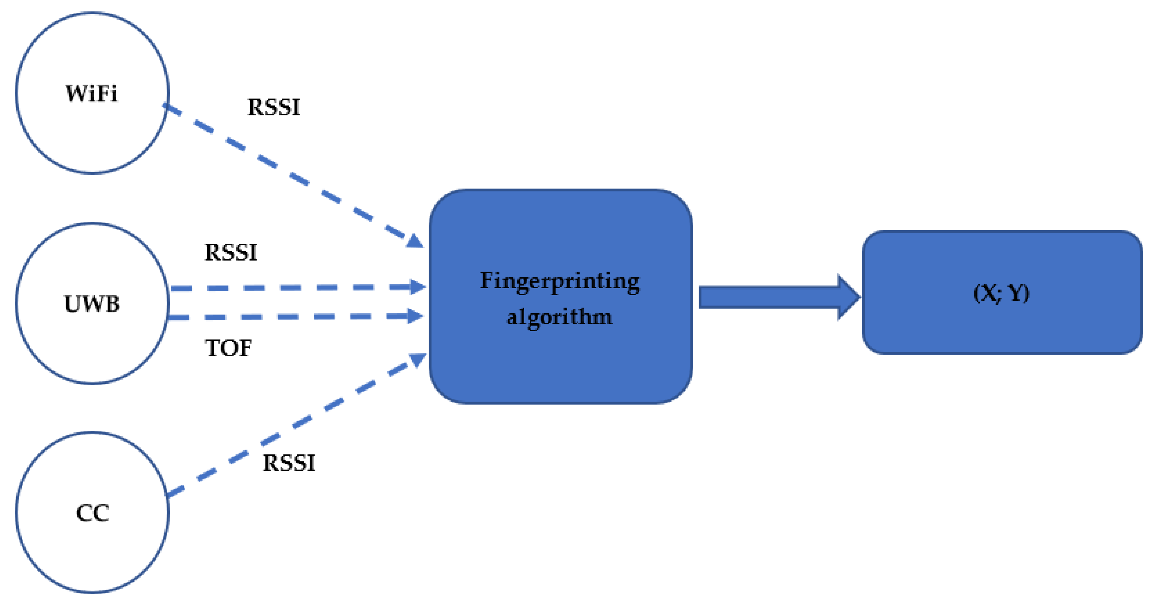
  • A novel fingerprinting-based approach is proposed, which utilizes the fusion of measurements collected using different technologies, namely WiFi RSSI, ultra-wideband RSSI, ultra-wideband time of flight and RSSI in the 433 MHz frequency band;
  • The proposed method is validated using measurements collected with four different technologies in a setup containing five access points (APs). The measurements are divided into learning and test points;
  • The fusion-based performance using the four technologies is evaluated for all 17 different combinations;
  • Three different widely used learning methods, namely the weighted K-nearest neighbor (WKNN), the random forest (RF) and the artificial neural network (ANN) are tested in the approach to examine which provides the best performance.
The remainder of the paper is organized as follows. In Section 2, related work is presented in addition to the methods and techniques used. Section 3 contains the presentation of the measurement system. The tested algorithms are presented in Section 4. Section 5 contains the achieved results. Finally, Section 6 contains the conclusion and future work plans.

2. Related Works

In related works, several localization methods and wireless communication technologies can be found. Most studies apply RFID [21], WiFi [22,23,24,25,26], BLE [16,17,18], ZigBee [27,28] or UWB [12,13] technologies in communication-based indoor localization systems, but there are devices that operate on different frequencies and use another modulation. Most of the works applied only one technology. Numerous RSSI [22,23,24] and time-based [13] indoor localization methods were tested. In these cases, the position can be estimated using fingerprinting or trilateration. Several methods are available for fingerprinting-based positioning. The methods that are widely used include support vector machine (SVM) [54], RF [18], KNN [26], WKNN [24], and ANN [28].
The emitted radio wave loses its strength as it propagates in free space. The amount of loss depends on the distance. The name of this model is the FSPL model. Signal propagation is affected by several factors. These include temperature, reflection, obstacles, and humidity. This is described by the Friis outdoor transmission equation [55]:
P r e c ( d ) = P t x · G t · G r · λ 2 ( 4 · π ) 2 · d 2 · L ,
where P r e c ( d ) represents the power of the signal at distance d , P t x is the power of the transmitter, G t and G r are the gain factors for the transmitter and the receiver antennas, λ is the wavelength, d is the distance between the transmitter and the receiver, and L denotes the factor for circuit losses.

2.1. WiFi

WiFi includes the most popular wireless local area network (WLAN) standards, which follows the Institute of Electrical and Electronics Engineers (IEEE) 802.11 standards. The range of the routers can be up to 100 m. Most of the technologies operate in the 2.4 GHz and the 5 GHz bands. The used modulation is the direct sequence spread spectrum (DSSS) or the orthogonal frequency division multiplexing (OFDM).
In [22], a MLNN network was used with multiple hidden layers. ESP8266 modules were used as APs. Several types of measurements were performed in the 12 m × 12 m room. First, the ESPs were placed in a matrix form every 6 m, then every 4 m and 3 m. The resolutions used during the measurements were 2 m, 1 m, and 0.5 m. A mobile phone was used to measure the RSSI values at the designated points. There were 300 data for teaching and 100 data for testing at each point. The highest accuracy was achieved with 25 AP, the value of the mean absolute error (MAE) was 0.46 m. Simulations were performed too, where the generated data achieved an accuracy of 0.23 m with 25 APs in a 10 m × 10 m area.
The authors of [23] used a recurrent neural network (RNN). The special feature of this network is that the previous outputs influence the current output, so a memory is needed. Six APs were used, RSSI was measured at 365 points and the network was tested at 175 points. WiFi RSSI was measured with a phone placed on a mobile robot, both in the 2.4 GHz band and in the 5 GHz band. The MAE value of the best achieved result is 0.75 m, which was obtained with two hidden layers and 100–100 neurons. In 80% of cases, the developed method produced an error of less than 1 m.
Previous work [24] reports a comparison of three different methods. The ANN, RF and WKNN performance were compared to each other. WiFi technology was chosen to make five heatmaps for five Aps. The room where the measurement was taken had an enclosing dimension of 3.6 m × 6.6 m. The heatmaps’ resolution was 20 cm. A total of 10 RSSI measurements per points were performed, resulting to 50 values per point. For the error reduction, the 10 values were averaged. The accuracy of the localization was determined for two cases. In the first case the whole room was examined, in the second only LOS points were examined. The best results were produced by the neural network in both cases. It was followed by the WKNN and the RF method. The best result was 0.4816 m with the ANN. The ANN outperformed both the WKNN and the RF algorithms and provided significantly better performance.
The authors of [25] applied an SLFN network with the extreme learning machine (ELM) algorithm instead of traditional backpropagation (BP) methods. The advantage of this is that the teaching phase is faster and the chance of being stuck in a local minimum is lower. During the testing, robust principal component analysis (RPCA) was used for filtering the data. The environment where the proposed method was tested was an industrial robotics lab, with enclosure dimensions of 32 m and 16 m. The APs were placed at a height of 1.2 m. A total of 500 samples per anchor were taken at 107 points at every 1.2 m. The accuracy of the results was calculated using 30 test points and given as root mean square error (RMSE). The data collection took several months, which were pre-processed for teaching. With the proposed method, the RMSE value was 2.3054 m, while with the other methods they obtained a larger error.
The authors of [26] created an RSSI fingerprint database with a resolution of 5 m in a 30 m × 30 m room. The position was given by KNN and its weighted version, the WKNN method. In the case of KNN, the error was 1.5047 m, while in the case of WKNN it was 0.8323 m.

2.2. Radio Frequency Identification Technology

Radio frequency identification is a wireless radio-wave-based technology. There are two types of RFID systems, namely the passive and active systems. The passive systems’ big advantage is that they can operate without a power supply. They can operate only in small distances (1–2 m). In the active RFID systems, the tags have a battery. Their operating distance can reach 100 m. They can use several frequency bands, i.e., low frequency (LF), high frequency (HF) and ultra-high frequency (UHF); these versions can be distinguished [20].
The authors of [21] conducted an experiment with passive RFID tags. The tags were placed on the floor in a 13 × 19 matrix. The sensing surface of the tags was 43 mm × 43 mm. A robot was built to perform the localization. Multiple different scenarios were examined. The robot’s speed was changed between the measurements. The worst performance was when the robot moved quickly. In this case, four tags were not recognized. This means that the accuracy of the system was 90 mm.

2.3. Ultra-Wideband Technology

With UWB modules, localization can be performed with the help of the IEEE 802.15.4a. It operates on high frequencies, between 3.1 GHz and 10.6 GHz. The bandwidth of the channels is over 500 MHz. The most common ranging methods are the RSSI, TOA, AOA and TDOA measurement [15].
The authors of [12] measured the RSSI value in a 2 m × 2 m area using UWB technology in every 5 cm. The position was determined by least squares (LS) and with its improved version, sub-sampling least squares (SSLS). The obtained RMSE values are: 0.542 m and 0.330 m.
In [13], an UWB-based localization system was presented. Four anchor modules were used at different heights in a 5.3 m × 11.5 m room. The error was estimated with five test points. The time was measured, while the signal propagated between the transmitter and the receiver multiple times. It is the so-called symmetrical double-sided two-way ranging technique. The position was estimated with trilateration. The error was determined with Euclidean distance. Two scenarios were examined. In the first, all the points were LOS, while in the second, a person randomly moved in the area. The achieved accuracy was 11 cm with 2 cm precision.

2.4. Bluetooth and Bluetooth Low-Energy Technologies

Bluetooth (IEEE 802.15.1) is a short-range wireless communication standard. The first version was developed in 1994, since then it has developed a lot. It uses the same frequency band (2.4 GHz) as the WiFi so they can interfere. Its lower consumption version, the BLE, appeared in 2010. Its main advantage is the fast connection establishment between the modules [19].
In [16], BLE devices were used for indoor localization. The measurement was performed in a 9 m × 6 m office. The distance-RSSI function was determined using particle swarm optimization (PSO) and back-propagation neural network (BPNN). The position was given by the least squares method. The RMSE was 0.7018 m.
The authors of [17] measured RSSI values and round-trip time (RTT) using BLE modules. CC2650 modules and nRF52840 modules were used. Distances were calculated from the data obtained in this way, and then the position of the central module was determined. Two techniques were used simultaneously. The tests were carried out in a 15 m × 50 m room, where the position of a moving node was determined. With RSSI, the RMSE value was 5.69 m, while with the two techniques, the RMSE reduced to 2.78 m. The position was obtained from the distances. The average error was 2.34 m.
The reference [18] contains a random forest indoor localization technique. A total of 30 BLE beacons were used in the experiment. They achieved better results with random forest classifier than with the naïve Bayes. The random forest was 30% more accurate than naïve Bayes.

2.5. ZigBee and IEEE 802.15.4

The open ZigBee communication standard was developed by the ZigBee Alliance. It is based on the IEEE 802.15.4 standard. This standard is cost-effective, has low power consumption and is bidirectional. The network topology can be mesh, tree, or star. In the topology next to the repeaters and end devices are the coordinators to control the network. Its biggest advantage is that it can manage up to 65,000 devices.
Reference [27] investigated the fusion of RSSI and TOA techniques with CC2431 modules. A Kalman filter was used to estimate the distance. Several algorithms were investigated. These included averaging, neural networks, and weighting. The error value was 1.99 m with RSSI, 1.15 m with TOA, 0.82 m with averaging, 0.72 m with weighting, and 0.32 m with neural network.
In [28], an MLP ANN was proposed for localization. The type of communication was based on IEEE 802.15.4. The measurements were taken in a laboratory with enclosing dimensions of 6 m × 15 m. Five anchors were placed in the room and 500 values were measured every 60 cm at each point (100 measurements/AP), in a total of 240 points. The performance of the network was tested with different numbers of neurons and with different transfer functions (purelin, tansig, radial base, and resilient BP). The best achieved accuracy was 0.3 m.

2.6. Comparison of Different Technologies

Among the main technologies, UWB TOA provides the highest accuracy during localization, according to the references [56,57]. The biggest advantage of this system is that it works in a different frequency band than other technologies, which can often interfere with each other. The disadvantage of UWB is that it has higher costs than other technologies. The accuracy, advantages, and disadvantages of the technologies are listed in Table 1.

3. Experimental Setup

For preparing the measurement system, a large size laboratory room was chosen. Due to the equipment, many points were NLOS in this environment. In this room, RSSI-based fingerprints and one-time-based fingerprint were created using different wireless technologies that operate at different frequencies. The technologies chosen were WiFi, UWB, and technologies using a 433 MHz industrial, scientific, and medical (ISM) frequency bands.

3.1. Received Signal Strength Indication

The RSSI value of the incoming signal can be determined by the receiver after the signal has arrived. By transforming Equation (1), a logarithmic model can be determined, which describes how much energy is lost as a function of distance in Equation (2). P L ( d 0 ) is the path loss taken at the reference point, and N is the environmental factor. In most cases, the R S S I value is given in dBm, which means that it is compared to the 1   m W Equation (3). Using Equation (4), the distance can be expressed, which can be seen in Equation (5).
P L ( d ) [ d B ] = P L ( d 0 ) [ d B ] + 10 · N · l o g 10 ( d d 0 )
( d B m ) = 10 · l o g P ( m W ) 1   m W
R S S I = ( 10 · N · log ( d ) + A )
d = 10 ( R S S I + A 10 N )

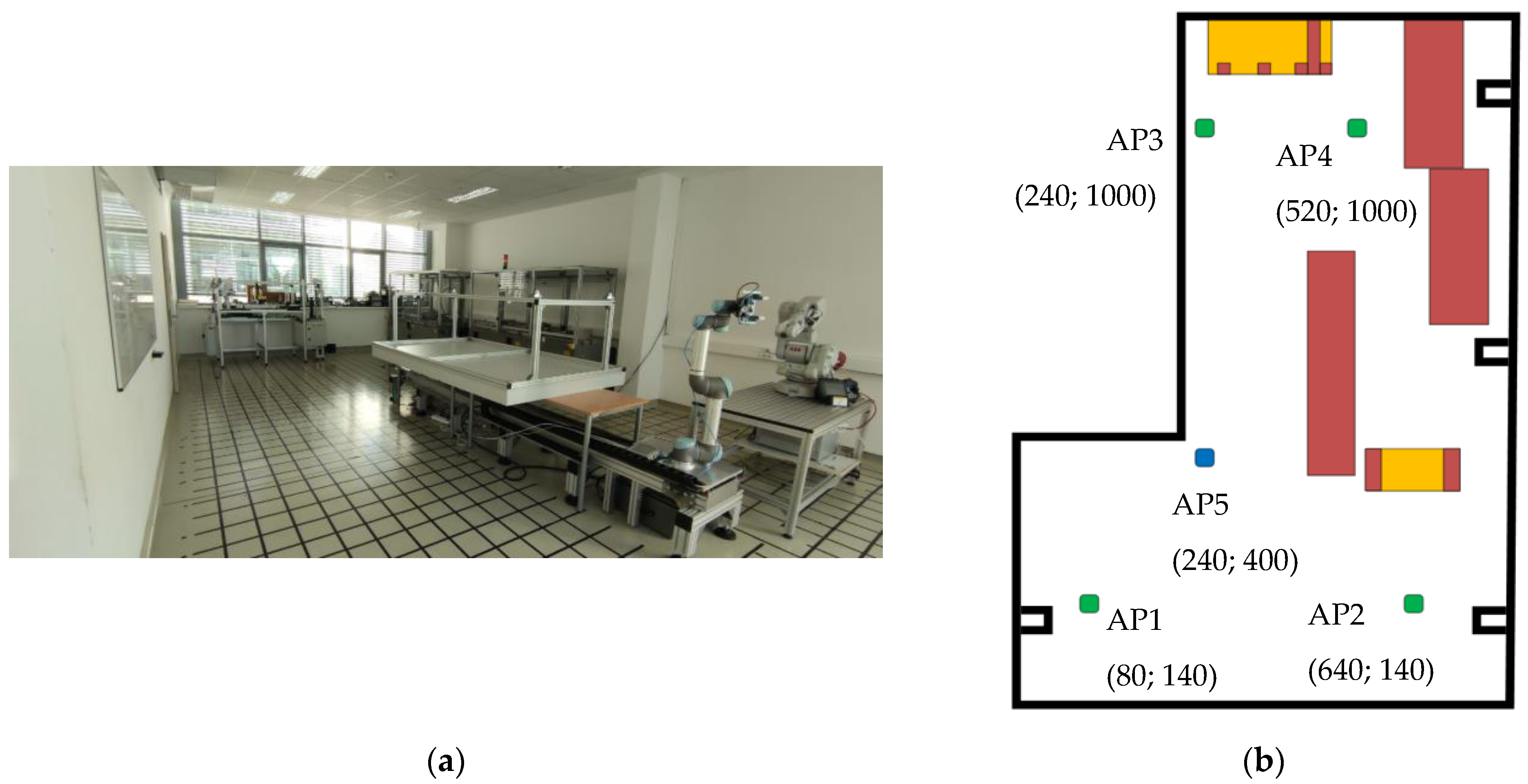
3.2. Measurement System

The data collection was performed in the Robotics Laboratory of the Faculty of Engineering, University of Szeged, which can be seen in Figure 1. The dimensions of the laboratory are 12 m × 8 m, which includes a separate storage room where no measurements were taken. The lab was rearranged for the duration of the measurements. The tables and chairs found here were taken out, and a larger field table was moved to increase the usable area for measurements. It is also important to mention that there are several larger devices and machines left in the room, which can affect the propagation and reflection of the signals. These devices are marked in red and orange colors in Figure 1. In addition, two sides of the room have almost full-length windows. After the rearrangement, the points required for fingerprinting were marked with insulating tape, by drawing lines parallel and perpendicular to the windows every 20 cm. The designated intersection points were the measurement points where RSSI and TOF values were measured during fingerprinting. There were a total of 1408 measurement points.
The anchors, i.e., modules with fixed coordinates, were tried to be near the corners of the room. The coordinates of the anchors in cm are as follows:
  • AP1 (80, 140);
  • AP2 (640, 140);
  • AP3 (240, 1000);
  • AP4 (520, 1000);
  • AP5 (240, 400).
The anchors were equipped with several modules. The WiFi technology was controlled by an ESP32 NodeMCU module. For the UWB technology, an ESP32UWB board was used, which is manufactured by Makerfabs and equipped with the DW1000 UWB module. It was used only in 4 out of the 5 anchors because of the limitation of the technology. AP5 did not contain this technology, which is marked with blue color in Figure 1. In the 433 MHz frequency band, the Texas Instrument’s CC1101 module was used. In four cases, the power supply of the modules was provided by the main electric network through an adapter, while in one case it was provided by a power bank.
Due to the high number of measurement points, the measurements were carried out by a mobile robot, which followed a total of 36 straight trajectories. The mobile robot had two ESP32 modules, one of which controlled the motors, and the other was responsible for the measurements. In addition, the CC1101 module and the ESP32UWB were also installed on it. Infra-red (IR) sensors were used for line following. The robot stopped at the intersections and made 10 measurements with all technologies. Altogether, 180 measurement values were collected per point (40 for UWB RSSI, 40 for UWB TOF, 50 WiFi RSSI, and 50 CC RSSI). The data were transmitted to a laptop using message queue telemetry transport (MQTT) communication.
In another 20 randomly chosen points, data were collected for testing the performance of the localization algorithm. Some of the points were in the NLOS position and some of them were under the tables.

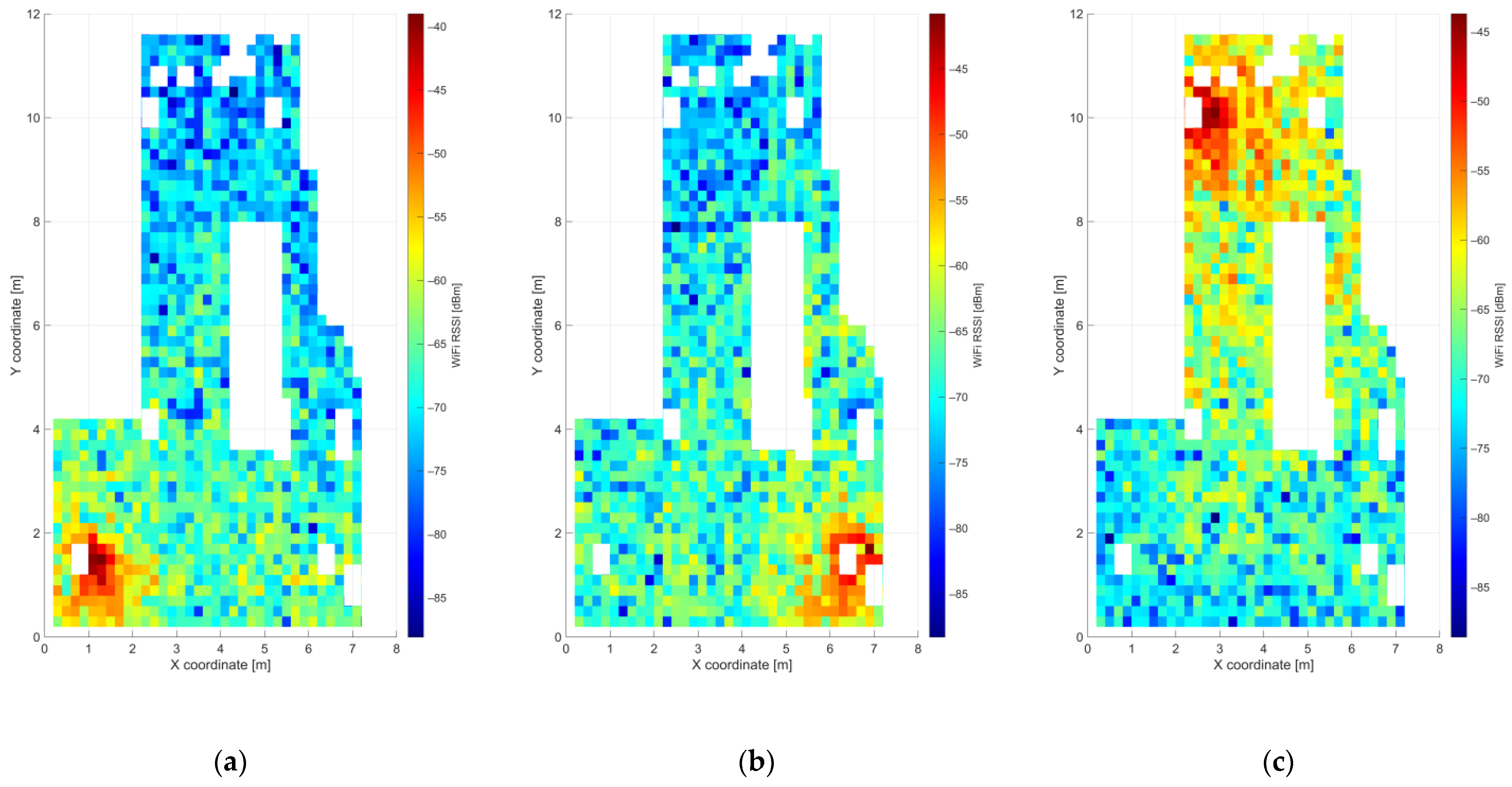
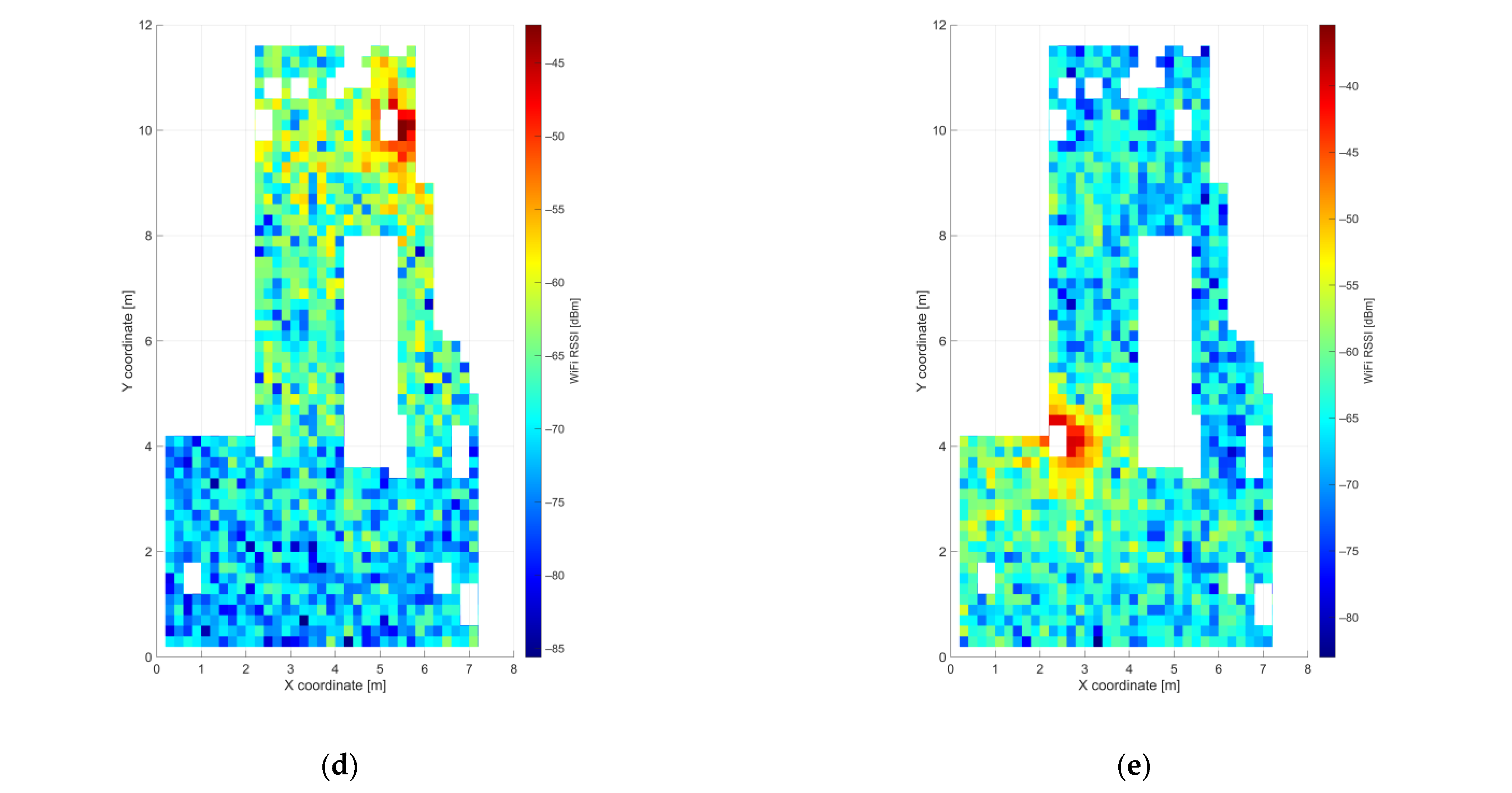
3.3. WiFi Received Signal Strength Indication

Among the four types of investigated technologies, WiFi was one those used to record the fingerprint in the room. The ESP32 on the mobile robot functioned as an AP. The ESP32 is a system on a chip (SoC), developed by the Espressif Systems. Xtensa LX6 contains a 240 MHz dual core microcontroller. It supports IEEE 802.11b/g/n data transfer protocols and Bluetooth 4.2. It supports both “Station” and “SoftAP” modes, which can be used simultaneously. It can communicate with I2C, SPI, and UART. The anchors worked in station mode. When the robot reached an intersection, it sent a signal to the stations, which measured RSSI every 100 ms a total of 10 times.
The RSSI values were between −88.6 dBm and −35.4 dBm. Figure 2 shows the heatmap for the 5 anchors. The heatmaps were created by averaging the 10 measured values to decrease the effect of noise. Dedicated parts where measurements could not be taken due to obstacles such as location of the storage room, columns, anchors, linear drive, and other machines, are marked with white color on the maps. The places with stronger signal, i.e., with a higher RSSI value, are marked with red color, while the places with weaker signal are marked with blue color.

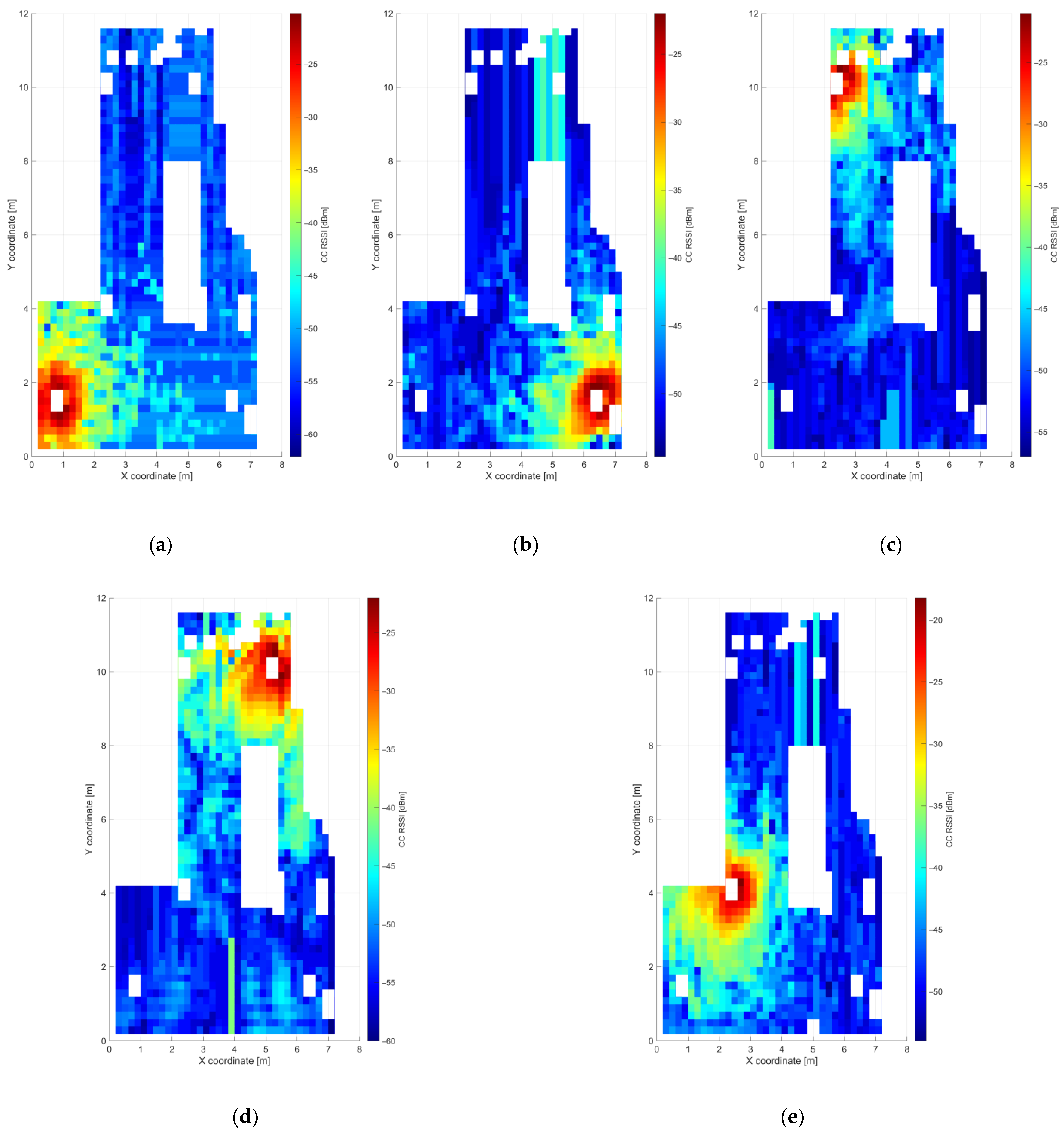
3.4. CC Received Signal Strength Indication

The CC1101 radio frequency transceiver was developed by Texas Instruments. It can also use several frequency bands: 315 MHz, 433 MHz, 868 MHz, and 915 MHz. It can use several frequency modulation methods: 2-FSK, 4-FSK, GFSK, MSK, OOK, and ASK. Its consumption is extremely favorable, very low. It uses SPI—serial peripheral interface communication protocol. The receiver can filter the data packets by monitoring the address and monitoring the length of the message and CRC. At the end of the data package, the package manager on the customer side can add 2 additional status bits, which contain the CRC status, the LQI—link quality indicator—and the RSSI value. It can provide the RSSI value with a resolution of 0.5 dBm.
In this case, the RSSI values were in the range of −62.1 dBm and −18.2 dBm. The heatmaps shown in Figure 3 were prepared in a similar way as in the case of Figure 2. Blue values mean a weaker signal, while red values mean a stronger one. In some cases large homogeneous blue areas can be seen, which means a weaker signal, or that there was no big change in the RSSI value.

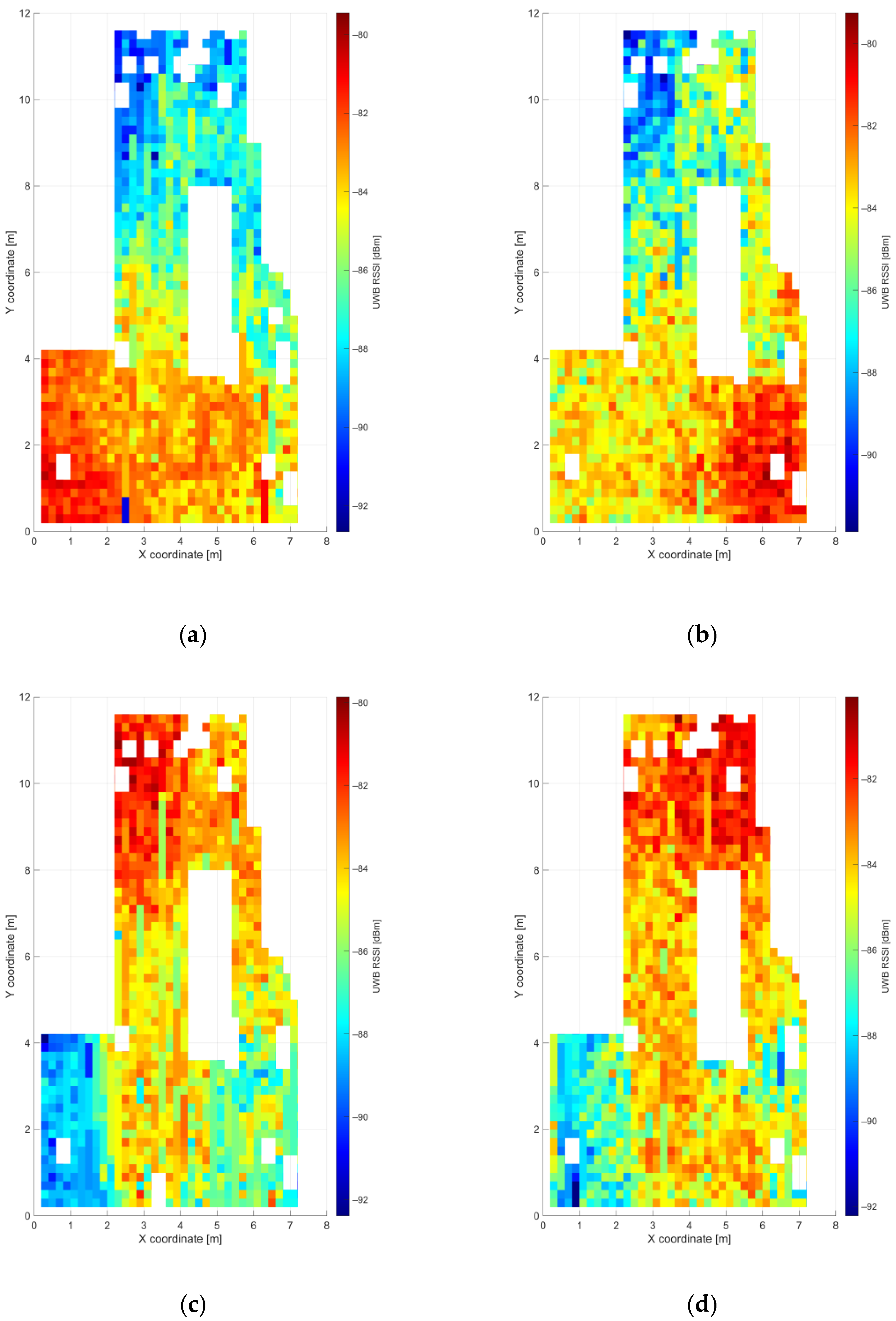
3.5. Ultra-Wideband Received Signal Strength Indication

The third type of heatmap was created using the ESP32UWB modules created by Makerfabs. These boards have DW1000 UWB modules in addition to an ESP32. The two devices can communicate using SPI. Modules can function as both anchors and tags. They support 4 RF frequency bands from 3.5 GHz to 6.5 GHz. The tags can communicate with several anchors and measure distances. Both anchors and members can specify the RSSI to two decimal places. In this case, the robot was the member to which the four anchors were connected. This module also measured RSSI and time (distance).
In this case, the RSSI values were in the range of −92.66 dBm −79.259 dBm, which is quite small compared to the other 2 methods. The heatmaps can be seen in Figure 4. Blue values mean a weaker signal, while red values mean stronger signal strength.

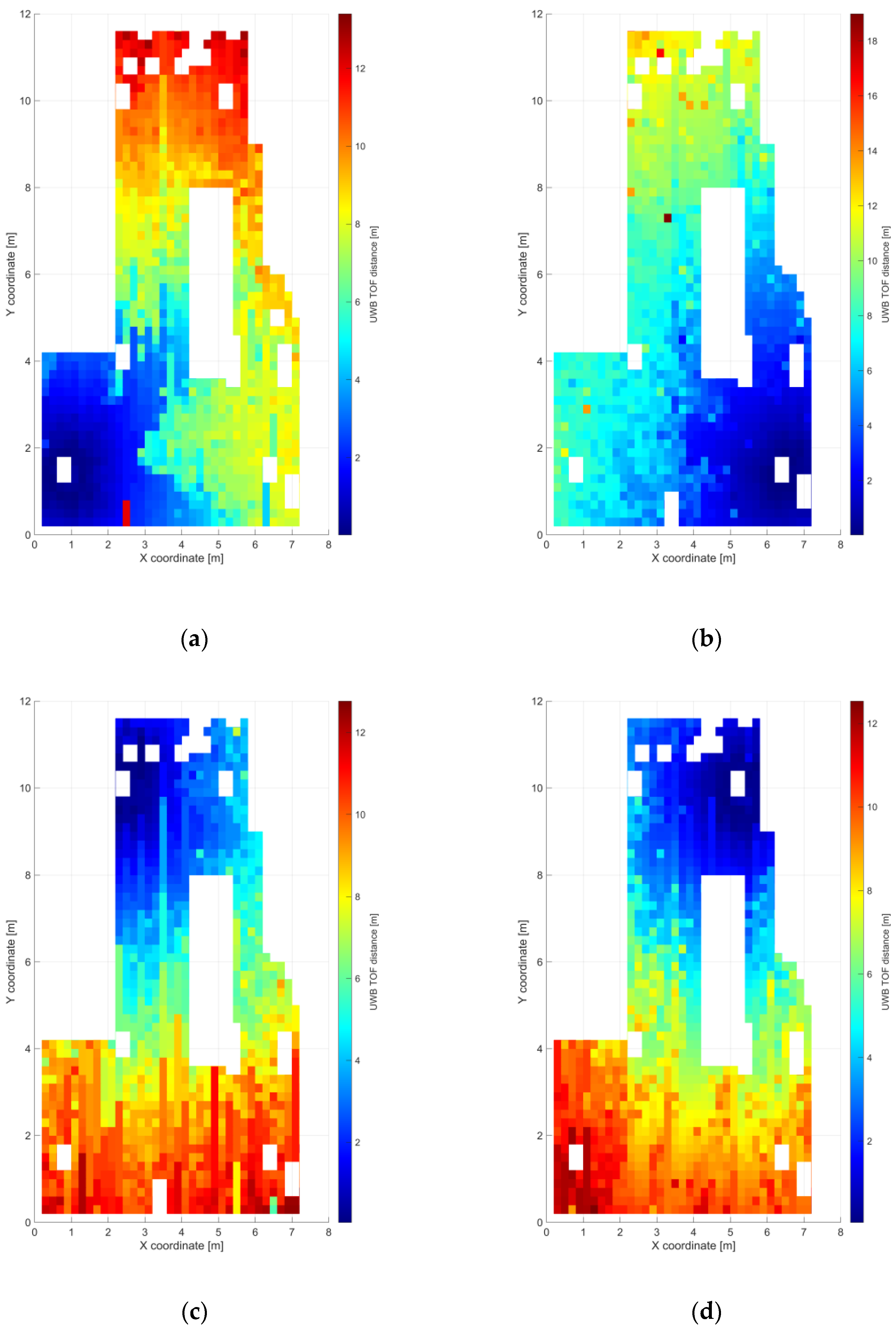
3.6. Ultra-Wideband Time of Flight

In addition to measuring RSSI, the ESP32UWB modules can also measure time. From the measurement of time, the distance between the modules can be determined using the propagation speed of the signal. The DW1000 module allows the use of both TOF and TDOA. In this case, the module measured the TOF.
The TOF values were between 0.0138 and 18.9860 m during the experiment. Figure 5 shows the related maps. The closer the anchor is, the bluer the figure is, and the farther away it is, the redder is. In the few places shown in the figures, there is a homogeneous red area, which is an error that was filtered out during the training of the network.

4. Proposed Fingerprinting-Based Method

It can be noticed from the heatmaps that the data are different at the four types of technologies. One carries extra information compared to the other, which can be used to increase the accuracy of localization. The position can be determined with different fingerprinting-based methods. These methods are WKNN, RF, and ANN. These work from a database, i.e., from the fingerprinting. The proposed localization method can be seen in Figure 6. The localization algorithm uses RSSI and TOF values to determine (X; Y) coordinates. The RSSI and TOF values can be used at the same time or separately.

4.1. Tested Fingerprinting Algorithms

The tested methods included one of the simplest fingerprinting-based algorithms, the WKNN, the RF method, and the ANN.

4.1.1. Weighted K-Nearest Neighbor

The WKNN algorithm is an improved version of the KNN algorithm that uses weighting. This is one of the simplest fingerprinting localization techniques. The simplest version is when K = 1, and the vector of the input and measured values are compared with the vectors belonging to individual points in the database, and then the most similar one is selected. By increasing K, the most similar K position is selected, and then the estimated position is obtained by averaging the coordinates. At WKNN, the weighted average is based on similarity. The algorithm is detailed in [58].
In the first step the Euclidean distance ( E D ) is determined
E D i , j = m = 1 M ( F P i m F P j m ) 2 ,
where M is the number of anchors, F P i m   and F P j m are the vectors belonging to the anchor m in the ith point and the fingerprinting vector from the database’s j th point, respectively. The fingerprint vectors were normalized to a range between 0 and 1, since the proposed method applies measurements of different technologies, which provide measurements in different ranges.
The next step is to determine the smallest distance
d r , u = m i n { E D i , j } ,
where E D i , j is the distance between u measurement point and r reference point.
The following step is to calculate w k weights as
w k = 1 d r , u 2       ( k = 1 , , K ) ,
The calculated coordinates are given as
x ^ =   k = 1 K ( w k · x k ) k = 1 K w k ,
y ^ = k = 1 K ( w k · y k ) k = 1 K w k ,
where x ^ and y ^ represent the calculated x and y coordinates; x k and y k are the K most similar points’ coordinates.
The similarity can be investigated using RSSI or TOF. In Equation (7), TOF or RSSI values can be placed or the combination of different technologies can be placed. Using Equation (7), the similarity between the points was determined. In the next step, the positions were put in ascending order according to similarity. Then, the first K points were selected. The weighted average of these points’ X and Y coordinates were taken. Equation (9) was used to determine the weights.

4.1.2. Random Forest

The random forest algorithm is a classification and regression procedure. It contains large number of decision trees with different structures. The decision making is performed with the help of the trees. The output can be created by averaging the trees’ outputs or by a majority vote. One of its advantages is that it generates decision trees randomly. This is achieved using the so-called bootstrap aggregation (i.e., bagging). Bagging means that the training set is modified randomly at each tree. Its disadvantages include the fact that the algorithm is slow and often complex because of the generation of the large number of decision trees. Another disadvantage is that the model can overlearn.
Firstly, the decision trees should be created. During the creation, the bagging was applied. The inputs, i.e., the RSSI and TOF values, must be arranged in a specific structure, and then the algorithm generalizes multi-level decision trees with the help of the corresponding outputs. The performance of the method was tested with several numbers of decision trees. In the phase of testing, the output X and Y coordinates were given with the weighted sum of the outputs of the trees.

4.1.3. Artificial Neural Networks

There have been many studies on RSSI-based localization with neural networks recently. Many types of networks have been tried and mixed with other techniques. Among the most common is the multi-layer perceptron (MLP) [28], e.g., the single hidden layer feedforward neural network (SLFN) [25] (a neural network containing one hidden layer, spreading forward), but also the perceptron containing more hidden layers and the RNN [23] are also typical.
ANN imitates the functioning of the human brain. The basic unit of these is the neuron, which is connected within the network and operates according to some logic that the external observers do not necessarily know. One of the most common types of neural network is the MLP. It is a feedforward neural network, which means that the signal propagates in one direction, the outputs are not connected to each other, the input layer only forwards the signal, and there can be any number of hidden layers (often only one is used). They can be built from three types of layers, which are the input layer, hidden layer, and output layer. The individual layers are arranged vertically, parallel to each other. In the hidden layer, the weighted sum and linear combination of the excitations appear at the input point of the neurons:
s i ( l ) = j p r e d ( i ) y j ( l 1 ) · w j i ( l 1 ) + b i ( l 1 ) ,
where p r e d ( i ) neurons preceding the i th unit, s i ( l ) is the linear combination of inputs, l th layer, i th neuron, y j ( l 1 ) is the output of the j th neuron of the ( l 1 ) st layer, w j i ( l 1 ) is the weight between the j th neuron of the ( l 1 ) st layer and the i th neuron of the lth layer, and b i ( l 1 ) is the bias value belonging to the i th neuron of the l th layer, which is used to ensure that the network gives an output even if the input is 0.
The task of the neuron is to process its input with the help of its activation function. The most widely used activation functions are the sigmoid and the linear functions. The networks are mostly trained offline, where the weights between the neurons are modified based on inputs with corresponding target values in the output layer until an exit condition is reached. Several methods can be used when training the network. Among the more widespread is backpropagation.
In this case, the data arriving at the input layer of the neural network are the RSSI and/or TOF values that can be measured at the given position. There are several neurons in the hidden layer. The neural network was examined with several numbers of neurons. The activation function of these neurons is tangent sigmoid. The output layer has two members that are responsible for providing the X and Y coordinates.

5. Results

In the evaluation process, several cases were examined with all three localization methods. All possible combination of the applied four technologies were tested. This covered a total of 15 cases. There were four cases when the four types of technologies were examined separately, in six cases, two technologies; in four, cases three technologies, and in one, case four technologies were combined. The tested combinations are the following:
1.
CC RSSI;
2.
WIFI RSSI;
3.
UWB RSSI;
4.
UWB TOF;
5.
CC RSSI + UWB TOF;
6.
CC RSSI + UWB RSSI;
7.
CC RSSI + WIFI RSSI;
8.
UWB RSSI + WIFI RSSI;
9.
UWB RSSI + UWB TOF;
10.
UWB TOF + WIFI RSSI;
11.
CC RSSI + UWB TOF + WIFI RSSI;
12.
CC RSSI + UWB TOF + UWB RSSI;
13.
CC RSSI + UWB RSSI + WIFI RSSI;
14.
WIFI RSSI + UWB TOF + UWB RSSI;
15.
UWB RSSI + CC RSSI + UWB TOF + WIFI RSSI.
The three tested methods were examined with several parameters, which can be seen in Table 2. When applying the WKNN algorithm, the positioning was performed by changing the value of K between 1 and 10 for the test points. Applying the RF method, the number of trees was changed, i.e., it was 2/5/10/50/100/150/200 during the testing. The decision trees’ type was regression, and the predictor was selected with curvature. When the localization was performed with ANN, the number of neurons was between 1 and 100. The training set was divided into two smaller groups. The first one was the training set, which included 70% of the data. The other group contained 30% of the data, which was used for validation. The training function during the training was the Levenberg–Marquardt method. The maximum number of iterations was set to 5000, the performance goal was set to 0, and the performance of the network was calculated with mean squared error (MSE).
The MAE and the standard deviation (STD) were used as performance metrics, which can be calculated using Equations (10) and (11), respectively. The error was given by 20 test points that were randomly selected.
M A E = 1 N i = 1 N ( x ^ i x i ) 2 + ( y ^ i y i ) 2 ,
S T D = 1 N 1 i = 1 N | A i M A E | 2 ,
A i = ( x ^ i x i ) 2 + ( y ^ i y i ) 2 ,
where x ^ i and y ^ i are the estimated positions of the i th point, x i and y i are the real positions, N is the number of points and A i represents the observations in the point i , i.e., the error of point i in Equation (12).

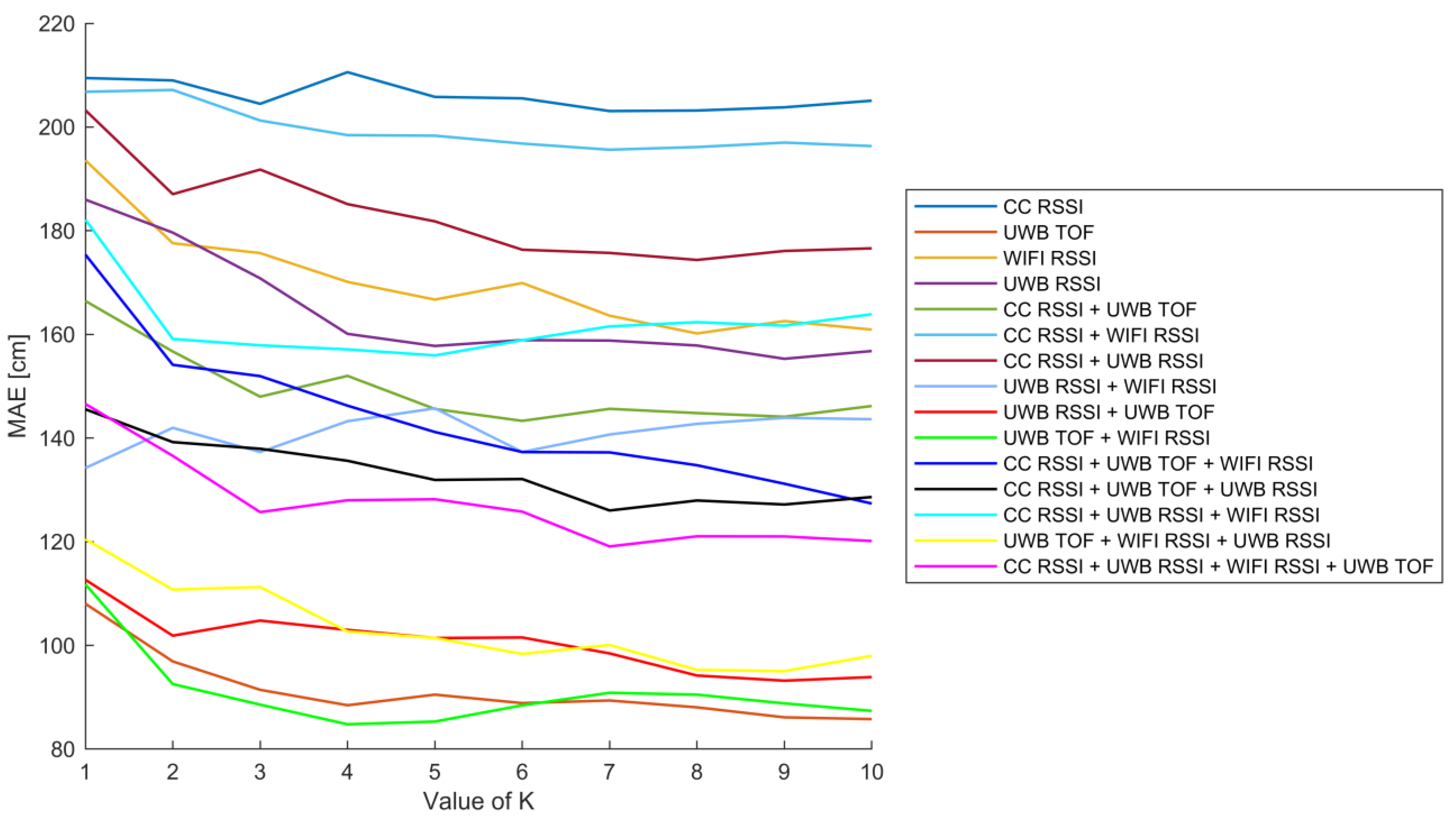
5.1. Results Using Weighted K-Nearest Neighbor

The RSSI and distance range for some technologies, which affects the weights in WKNN, as can be seen in Section 3. For this reason, all types of data were separately normalized between 0 and 1. The best results for the 15 different cases with the WKNN algorithm are summarized in Table 3. The best result was given by the UWB TOF + WIFI RSSI case, when the localization accuracy was 84.78 cm. The case of UWB TOF + WIFI RSSI gave a better result with 1 cm, compared to UWB TOF. It can be observed that the best result is obtained when K = 4 for UWB TOF + WIFI RSSI. For WKNN, the fusion of UWB RSSI + WIFI RSSI provides better results than the original two technologies, i.e., WIFI RSSI and UWB RSSI. In the case of using UWB RSSI, a WIFI RSSI, the localization accuracy was 134.23 cm, which is a 21 cm, or 14% improvement compared to UWB RSSI.
The effect of increasing value K can be seen in Figure 7. It is noticeable that increasing this value provides better results. In 11 cases the best results were given when the value of K was 7 or higher.

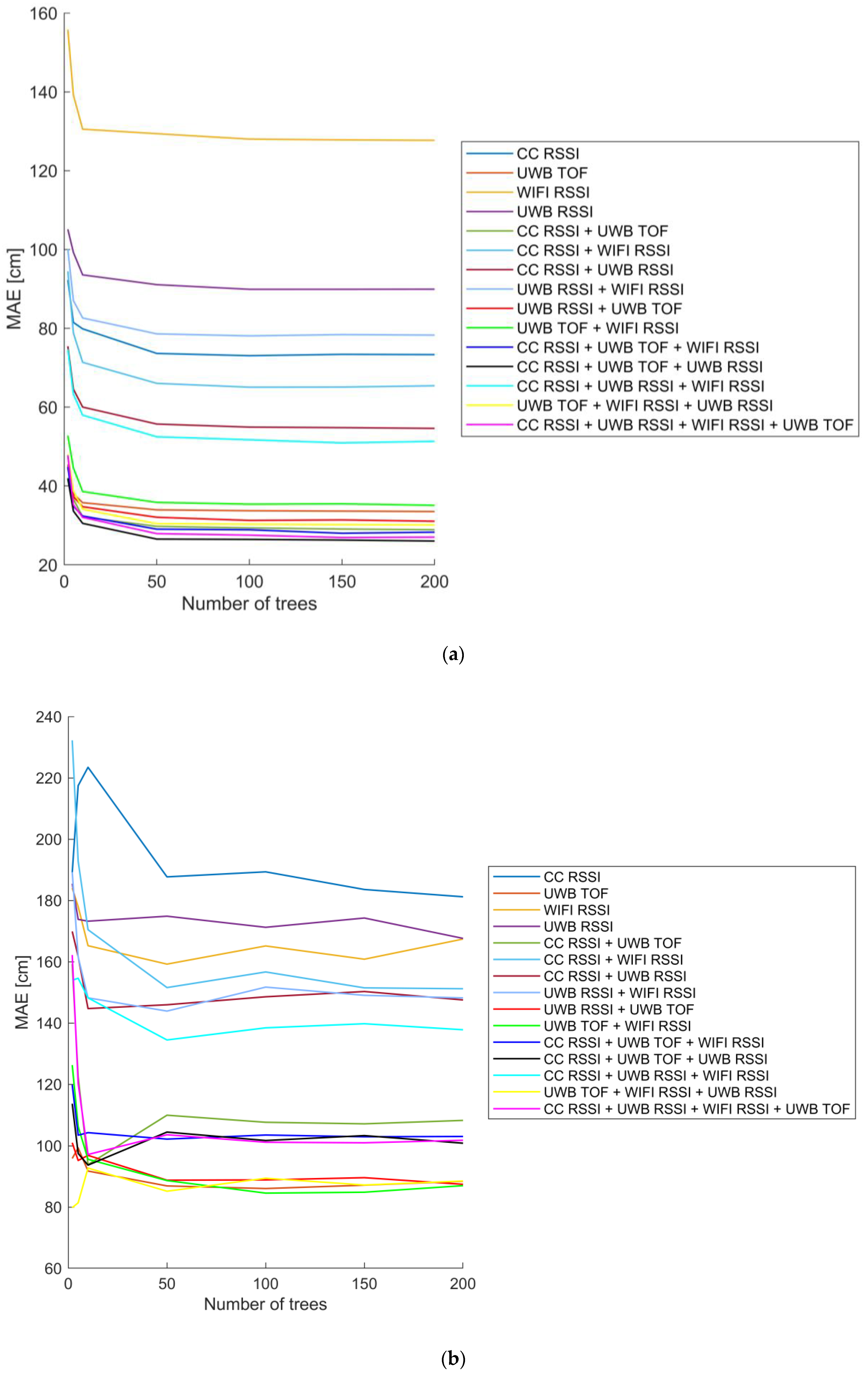
5.2. Results Using Random Forest

The random forest algorithm was evaluated with different numbers of trees for all defined combinations. The results are summarized in Table 4. Using each technology separately, the UWB TOF gave the best results. In this case, the MAE was 86.07 cm when testing with the 20 test data, and 33.70 cm when testing with the training data. In the case that only WIFI RSSI, CC RSSI, and UWB RSSI were used, this error increases by almost twice as much in each case. Examining two technologies provides better almost in every case than when applying only one technology. The improvement in the case of the fusion of CC RSSI and WIFI RSSI is 8 cm, i.e., 5% improvement compared to WIFI RSSI when using test data, and 8 cm, i.e., 11% improvement when testing with training data. For CC RSSI and UWB RSSI, the improvement is 23 cm, i.e., 14% improvement compared to UWB RSSI when using test data. The accuracy improved further in two cases, compared to cases with two technologies. These cases are: CC RSSI + WIFI RSSI + UWB RSSI, when the MAE value was 134.48 cm. The best overall result was provided by WIFI RSSI + UWB TOF + UWB RSSI, when the MAE was 79.84 cm. It is 7 cm or about 8% improvement compared to UWB TOF in the case of testing with the 20 points. The best overall result was given in the case of applying training data, when CC RSSI was combined with UWB TOF and UWB RSSI. In this case, the MAE was 30.50 cm.
The effect of increasing the number of trees in the algorithm can be seen in Figure 8. It is noticeable that the more trees it contains the more accurate it is. In 4–4 cases the best result was obtained with 50 and 200 trees when the evaluation was performed on the training data.

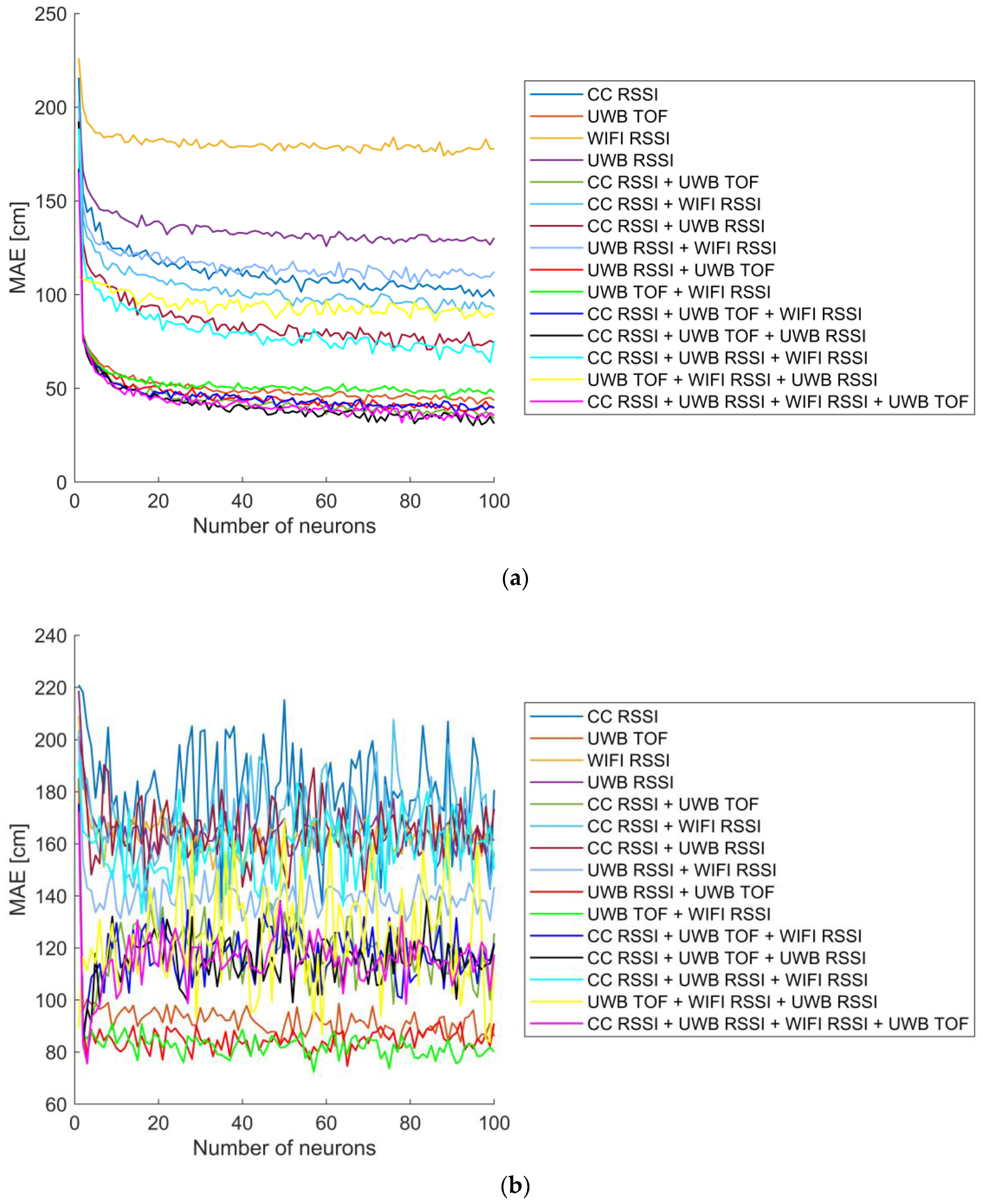
5.3. Results Using Artificial Neural Network

While examining the neural network, several different cases were tested. The number of neurons in the hidden layer was varied between 1 and 100. For each number of neurons, the evaluation was performed five times for both the test points and training data. The best training result was considered.
The results of evaluating the test data are summarized in Table 5. It is noticeable that when only 1–1 technology was used the best result was provided by UWB TOF with 80.08 cm. The combination of two technologies resulted in improvement in some cases. Combining WIFI RSSI and CC RSSI the MAE was 9 cm smaller than when only CC RSSI was used. In the cases of combining three technologies, the UWB RSSI + WIFI RSSI + CC RSSI provided better results. Overall, the best result was provided with the fusion of UWB TOF and WIFI RSSI, when the error was 72.41 cm. This is a significant improvement over the UWB TOF error of 80.08 cm. It means 9.5% improvement.
The results of the testing on the training data are included in Table 5. When only one technology was used, UWB TOF provided the best results, with 41.69 cm, while the worst result was provided by WIFI RSSI, when the MAE value was 174.04 cm. The localization accuracy improved in almost all cases, except for UWB TOF + WIFI RSSI and WIFI RSSI + UWB TOF + UWB RSSI. The combination of two technologies resulted in improvement almost in every cases. By combining the two low-cost technologies (the CC RSSI and the WIFI RSSI) the improvement was about 9 cm, which means 9% improvement. The best result was obtained by using UWB TOF, CC RSSI, and UWB RSSI together, when the value of the localization error was 30.23 cm. This is a significant improvement of 10 cm compared to the UWB TOF error. It means a 24% improvement compared to the UWB TOF.
By increasing the number of neurons in the hidden layer, the accuracy of the neural network improved. This improvement can be seen in Figure 9. This figure contains the results of all cases. It is noticeable that the WIFI RSSI, the UWB RSSI, and the CC RSSI provided the worst results. The fusion of these technologies provided significantly better results.

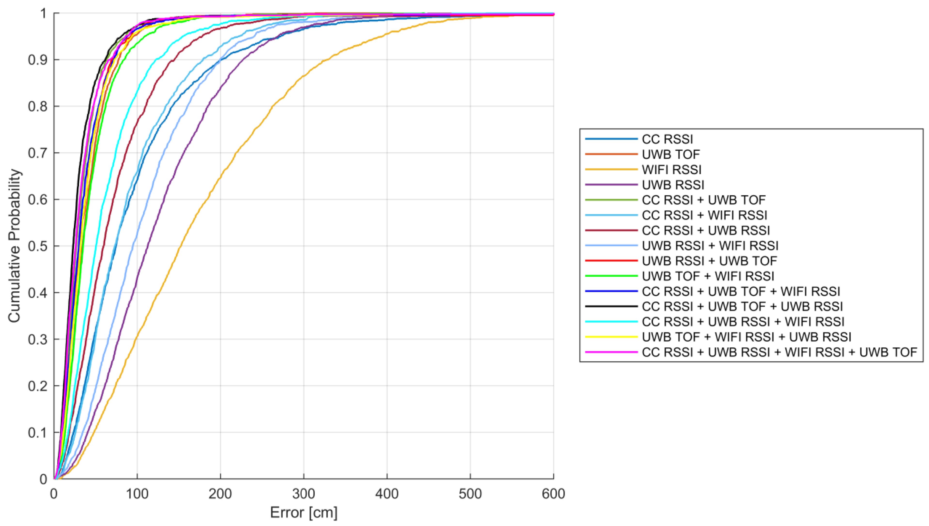
5.4. Comparison of Different Cases

In all cases, the neural network provided the best results when the evaluation was performed with the test data. The best overall results were provided by the RF and ANN when the evaluation was performed with the training data. The best results were obtained with the fusion of CC RSSI, UWB RSSI, and UWB TOF, when the localization error was 30.23 cm. The fusion of different technologies can significantly improve the accuracy of the localization. When using only the UWB module with the two technologies (UWB RSSI and UWB TOF), the error reduced to 31.04 cm from 33.70 cm. It is an 8% improvement compared to UWB TOF. Using the two other technologies, the best achieved result was produced by RF, when the MAE was 65.42 cm. This is almost an 11% improvement compared to CC RSSI and almost 50% compared to WIFI RSSI. The best result achieved by fusing the three RSSIs was also given by RF. At that time, the MAE was 54.48 cm, which is a 26% improvement over CC RSSI, a 17% improvement over UWB RSSI, and a 58% improvement over WIFI RSSI.
The cumulative distribution function (CDF) of errors for the best results in the case of training data can be seen in Figure 10. The errors larger than 600 cm were around 600 cm for the better visibility. The diagram shows that the error values are smaller in the cases when multiple technologies were used for localization.

6. Conclusions

In this paper, fingerprints were recorded with sensors using different frequency bands. The evaluation was carried out using several fingerprinting techniques. Among them were the WKNN, ANN, and RF algorithms. The algorithms were tested with several parameters. For the evaluation, 20 test points were used that were not included in the fingerprint. These test points were taken randomly. There are more under the tables and in places where not all points are LOS.
From the results it can be concluded that the RF and ANN outperform WKNN methods. Of the 15 examined combinations, when validated with the test points, the ANN provided the best results in every case. The best achieved result was provided by the fusion of UWB TOF, CC RSSI, and UWB RSSI, when the MAE value was 30.23 cm, which is a significant improvement of nearly 10% compared to the most accurate UWB TOF. With the fusion of the two low-cost technologies, CC RSSI and WIFI RSSI, the achieved improvement is 8 cm, i.e., 10%, compared to the more accurate CC RSSI. It can be noticed from these that the individual technologies complement each other and, with the selection of a suitable method (e.g., neural network or random forest), are suitable for improving localization.
Based on the presented results in [59], the performance of the proposed method could be further improved by increasing the number of anchors. The use of a node selection algorithm and an optimization-based method that can determine the density and the position of the anchors would also be reasonable. Based on the achieved results, adding further wireless technologies could further decrease the error rates. Future goals also include the fusion of other sensor types into the proposed method, which carry additional information.

Author Contributions

Conceptualization, D.C. and P.S.; methodology, D.C.; software, D.C., Á.O. and P.S.; validation, D.C.; formal analysis, D.C., Á.O. and P.S.; investigation, D.C., Á.O. and P.S.; resources, D.C., Á.O. and P.S.; data curation, D.C.; writing—original draft preparation, D.C.; writing—review and editing, Á.O. and P.S.; visualization, D.C. and P.S.; supervision, Á.O. and P.S.; project administration, Á.O. and P.S.; funding acquisition, Á.O. and P.S. All authors have read and agreed to the published version of the manuscript.

Funding

The work was supported by the National Research, Development, and Innovation Fund of Hungary through project no. 142790 under the FK_22 funding scheme.

Data Availability Statement

The data presented in this study are openly available at: https://github.com/csikdominik/RSSI-fingerprint-database (accessed on 17 January 2023).

Conflicts of Interest

The authors declare no conflict of interest.

References

  1. Asghari, P.; Rahmani, A.M.; Javadi, H.H.S. Internet of Things Applications: A Systematic Review. Comput. Netw. 2019, 148, 241–261. [Google Scholar] [CrossRef]
  2. Majid, M.; Habib, S.; Javed, A.R.; Rizwan, M.; Srivastava, G.; Gadekallu, T.R.; Lin, J.C.-W. Applications of Wireless Sensor Networks and Internet of Things Frameworks in the Industry Revolution 4.0: A Systematic Literature Review. Sensors 2022, 22, 2087. [Google Scholar] [CrossRef] [PubMed]
  3. Mao, G.; Fidan, B.; Anderson, B.D.O. Wireless Sensor Network Localization Techniques. Comput. Netw. 2007, 51, 2529–2553. [Google Scholar] [CrossRef] [Green Version]
  4. Mesmoudi, A.; Feham, M.; Labraoui, N. Wireless Sensor Networks Localization Algorithms: A Comprehensive Survey. IJCNC 2013, 5, 45–64. [Google Scholar] [CrossRef]
  5. Senouci, M.R.; Mellouk, A. Wireless Sensor Networks. In Deploying Wireless Sensor Networks; Elsevier: Amsterdam, The Netherlands, 2016; pp. 1–19. [Google Scholar]
  6. Chen, Y.; Li, X.; Ding, Y.; Xu, J.; Liu, Z. An Improved DV-Hop Localization Algorithm for Wireless Sensor Networks. In Proceedings of the 2018 13th IEEE Conference on Industrial Electronics and Applications (ICIEA), Wuhan, China, 31 May–2 June 2018. [Google Scholar]
  7. Paul, A.; Sato, T. Localization in Wireless Sensor Networks: A Survey on Algorithms, Measurement Techniques, Applications and Challenges. J. Sens. Actuator Netw. 2017, 6, 24. [Google Scholar] [CrossRef] [Green Version]
  8. Cheng, L.; Wu, C.; Zhang, Y.; Wu, H.; Li, M.; Maple, C. A Survey of Localization in Wireless Sensor Network. Int. J. Distrib. Sens. Netw. 2012, 8, 962523. [Google Scholar] [CrossRef]
  9. Han, G.; Jiang, J.; Zhang, C.; Duong, T.Q.; Guizani, M.; Karagiannidis, G.K. A Survey on Mobile Anchor Node Assisted Localization in Wireless Sensor Networks. IEEE Commun. Surv. Tutorials 2016, 18, 2220–2243. [Google Scholar] [CrossRef]
  10. Coluccia, A.; Fascista, A. A Review of Advanced Localization Techniques for Crowdsensing Wireless Sensor Networks. Sensors 2019, 19, 988. [Google Scholar] [CrossRef] [Green Version]
  11. Xu, R.; Chen, W.; Xu, Y.; Ji, S. A New Indoor Positioning System Architecture Using GPS Signals. Sensors 2015, 15, 10074–10087. [Google Scholar] [CrossRef] [Green Version]
  12. Wang, S.; Waadt, A.; Burnic, A.; Xu, D.; Kocks, C.; Bruck, G.H.; Jung, P. System Implementation Study on RSSI Based Positioning in UWB Networks. In Proceedings of the 2010 7th International Symposium on Wireless Communication Systems, York, UK, 19–22 September 2010; pp. 36–40. [Google Scholar]
  13. Silva, B.; Pang, Z.; Akerberg, J.; Neander, J.; Hancke, G. Experimental Study of UWB-Based High Precision Localization for Industrial Applications. In Proceedings of the 2014 IEEE International Conference on Ultra-WideBand (ICUWB), Paris, France, 1–3 September 2014; pp. 280–285. [Google Scholar]
  14. Alarifi, A.; Al-Salman, A.; Alsaleh, M.; Alnafessah, A.; Al-Hadhrami, S.; Al-Ammar, M.; Al-Khalifa, H. Ultra Wideband Indoor Positioning Technologies: Analysis and Recent Advances. Sensors 2016, 16, 707. [Google Scholar] [CrossRef] [Green Version]
  15. Mazhar, F.; Khan, M.G.; Sällberg, B. Precise Indoor Positioning Using UWB: A Review of Methods, Algorithms and Implementations. Wirel. Pers. Commun. 2017, 97, 4467–4491. [Google Scholar] [CrossRef]
  16. Li, G.; Geng, E.; Ye, Z.; Xu, Y.; Lin, J.; Pang, Y. Indoor Positioning Algorithm Based on the Improved RSSI Distance Model. Sensors 2018, 18, 2820. [Google Scholar] [CrossRef] [Green Version]
  17. Giovanelli, D.; Farella, E.; Fontanelli, D.; Macii, D. Bluetooth-Based Indoor Positioning Through ToF and RSSI Data Fusion. In Proceedings of the 2018 International Conference on Indoor Positioning and Indoor Navigation (IPIN), Nantes, France, 24–27 September 2018; pp. 1–8. [Google Scholar]
  18. Campana, F.; Pinargote, A.; Dominguez, F.; Pelaez, E. Towards an Indoor Navigation System Using Bluetooth Low Energy Beacons. In Proceedings of the 2017 IEEE Second Ecuador Technical Chapters Meeting (ETCM), Salinas, Ecuador, 16–20 October 2017; pp. 1–6. [Google Scholar]
  19. Mackensen, E.; Lai, M.; Wendt, T.M. Bluetooth Low Energy (BLE) Based Wireless Sensors. In Proceedings of the 2012 IEEE Sensors, Taipei, Taiwan, 28–31 October 2012; pp. 1–4. [Google Scholar]
  20. Zhou, J.; Shi, J. RFID Localization Algorithms and Applications—A Review. J. Intell. Manuf. 2009, 20, 695–707. [Google Scholar] [CrossRef]
  21. Tesoriero, R.; Tebar, R.; Gallud, J.A.; Lozano, M.D.; Penichet, V.M.R. Improving Location Awareness in Indoor Spaces Using RFID Technology. Expert Syst. Appl. 2010, 37, 894–898. [Google Scholar] [CrossRef]
  22. Dai, H.; Ying, W.; Xu, J. Multi-layer neural network for received signal strength-based indoor localization. IET Commun. 2016, 10, 717–723. [Google Scholar] [CrossRef]
  23. Hoang, M.T.; Yuen, B.; Dong, X.; Lu, T.; Westendorp, R.; Reddy, K. Recurrent Neural Networks for Accurate RSSI Indoor Localization. IEEE Internet Things J. 2019, 6, 10639–10651. [Google Scholar] [CrossRef] [Green Version]
  24. Csik, D.; Odry, A.; Sarcevic, P. Comparison of RSSI-Based Fingerprinting Methods for Indoor Localization. In Proceedings of the IEEE International Symposium on Intelligent Systems and Informatics (SISY), Subotica, Serbia, 15–17 September 2022. [Google Scholar]
  25. Cui, W.; Liu, Q.; Zhang, L.; Wang, H.; Lu, X.; Li, J. A Robust Mobile Robot Indoor Positioning System Based on Wi-Fi. Int. J. Adv. Robot. Syst. 2020, 17, 172988141989666. [Google Scholar] [CrossRef] [Green Version]
  26. Poulose, A.; Han, D.S. Performance Analysis of Fingerprint Matching Algorithms for Indoor Localization. In Proceedings of the 2020 International Conference on Artificial Intelligence in Information and Communication (ICAIIC), Fukuoka, Japan, 19–21 February 2020; pp. 661–665. [Google Scholar]
  27. Dong, Z.; Wu, Y.; Sun, D. Data Fusion of the Real Time Positioning System Based on RSSI and TOF. In Proceedings of the 2013 5th International Conference on Intelligent Human-Machine Systems and Cybernetics, Hangzhou, China, 26–27 August 2013; pp. 503–506. [Google Scholar]
  28. Gogolak, L.; Pletl, S.; Kukolj, D. Indoor Fingerprint Localization in WSN Environment Based on Neural Network. In Proceedings of the 2011 IEEE 9th International Symposium on Intelligent Systems and Informatics, Subotica, Serbia, 8–10 September 2011; pp. 293–296. [Google Scholar]
  29. Xie, H.; Gu, T.; Tao, X.; Ye, H.; Lv, J. MaLoc: A Practical Magnetic Fingerprinting Approach to Indoor Localization Using Smartphones. In Proceedings of the 2014 ACM International Joint Conference on Pervasive and Ubiquitous Computing, Seattle, WA, USA, 13 September 2014; pp. 243–253. [Google Scholar]
  30. Ouyang, G.; Abed-Meraim, K. A Survey of Magnetic-Field-Based Indoor Localization. Electronics 2022, 11, 864. [Google Scholar] [CrossRef]
  31. Hoeflinger, F.; Saphala, A.; Schott, D.J.; Reindl, L.M.; Schindelhauer, C. Passive Indoor-Localization Using Echoes of Ultrasound Signals. In Proceedings of the 2019 International Conference on Advanced Information Technologies (ICAIT), Yangon, Myanmar, 6–7 November 2019; pp. 60–65. [Google Scholar]
  32. Moutinho, J.N.; Araújo, R.E.; Freitas, D. Indoor Localization with Audible Sound—Towards Practical Implementation. Pervasive Mob. Comput. 2016, 29, 1–16. [Google Scholar] [CrossRef] [Green Version]
  33. Rahman, A.B.M.M.; Li, T.; Wang, Y. Recent Advances in Indoor Localization via Visible Lights: A Survey. Sensors 2020, 20, 1382. [Google Scholar] [CrossRef] [Green Version]
  34. Morar, A.; Moldoveanu, A.; Mocanu, I.; Moldoveanu, F.; Radoi, I.E.; Asavei, V.; Gradinaru, A.; Butean, A. A Comprehensive Survey of Indoor Localization Methods Based on Computer Vision. Sensors 2020, 20, 2641. [Google Scholar] [CrossRef]
  35. Wang, Y.-T.; Peng, C.-C.; Ravankar, A.; Ravankar, A. A Single LiDAR-Based Feature Fusion Indoor Localization Algorithm. Sensors 2018, 18, 1294. [Google Scholar] [CrossRef] [Green Version]
  36. de Sá, A.O.; Nedjah, N.; de Macedo Mourelle, L. Distributed Efficient Localization in Swarm Robotic Systems Using Swarm Intelligence Algorithms. Neurocomputing 2016, 172, 322–336. [Google Scholar] [CrossRef]
  37. Al-Sadoon, M.A.G.; Asif, R.; Al-Yasir, Y.I.A.; Abd-Alhameed, R.A.; Excell, P.S. AOA Localization for Vehicle-Tracking Systems Using a Dual-Band Sensor Array. IEEE Trans. Antennas Propagat. 2020, 68, 6330–6345. [Google Scholar] [CrossRef]
  38. Cao, S.; Chen, X.; Zhang, X.; Chen, X. Combined Weighted Method for TDOA-Based Localization. IEEE Trans. Instrum. Meas. 2020, 69, 1962–1971. [Google Scholar] [CrossRef]
  39. Gao, M.; Yu, M.; Guo, H.; Xu, Y. Mobile Robot Indoor Positioning Based on a Combination of Visual and Inertial Sensors. Sensors 2019, 19, 1773. [Google Scholar] [CrossRef] [Green Version]
  40. Chen, Y.; Chen, W.; Zhu, L.; Su, Z.; Zhou, X.; Guan, Y.; Liu, G. A Study of Sensor-Fusion Mechanism for Mobile Robot Global Localization. Robotica 2019, 37, 1835–1849. [Google Scholar] [CrossRef]
  41. Jiang, P.; Chen, L.; Guo, H.; Yu, M.; Xiong, J. Novel Indoor Positioning Algorithm Based on Lidar/Inertial Measurement Unit Integrated System. Int. J. Adv. Robot. Syst. 2021, 18, 172988142199992. [Google Scholar] [CrossRef]
  42. Hashim, H.A. Exponentially stable observer-based controller for VTOL-UAVs without velocity measurements. Int. J. Control 2022. [Google Scholar] [CrossRef]
  43. Li, C.; Wang, S.; Zhuang, Y.; Yan, F. Deep Sensor Fusion Between 2D Laser Scanner and IMU for Mobile Robot Localization. IEEE Sens. J. 2021, 21, 8501–8509. [Google Scholar] [CrossRef]
  44. Hashim, H.A.; Eltoukhy, A.E.E. Landmark and IMU Data Fusion: Systematic Convergence Geometric Nonlinear Observer for SLAM and Velocity Bias. IEEE Trans. Intell. Transport. Syst. 2022, 23, 3292–3301. [Google Scholar] [CrossRef]
  45. Hashim, H.A.; Abouheaf, M.; Abido, M.A. Geometric Stochastic Filter with Guaranteed Performance for Autonomous Navigation Based on IMU and Feature Sensor Fusion. Control Eng. Pract. 2021, 116, 104926. [Google Scholar] [CrossRef]
  46. Abu-Mahfouz, A.M.; Hancke, G.P. Localised Information Fusion Techniques for Location Discovery in Wireless Sensor Networks. Int. J. Sens. Netw. 2018, 26, 12–25. [Google Scholar] [CrossRef] [Green Version]
  47. Meng, T.; Jing, X.; Yan, Z.; Pedrycz, W. A Survey on Machine Learning for Data Fusion. Inf. Fusion 2020, 57, 115–129. [Google Scholar] [CrossRef]
  48. Aguerri, I.E.; Zaidi, A. Distributed Variational Representation Learning. IEEE Trans. Pattern Anal. Mach. Intell. 2021, 43, 120–138. [Google Scholar] [CrossRef] [Green Version]
  49. Moldoveanu, M.; Zaidi, A. In-Network Learning for Distributed Training and Inference in Networks. In Proceedings of the 2021 IEEE Globecom Workshops (GC Wkshps), Madrid, Spain, 7–11 December 2021; pp. 1–6. [Google Scholar]
  50. Moldoveanu, M.; Zaidi, A. On In-Network Learning. A Comparative Study with Federated and Split Learning. In Proceedings of the 2021 IEEE 22nd International Workshop on Signal Processing Advances in Wireless Communications (SPAWC), Lucca, Italy, 27–30 September 27 2021; pp. 221–225. [Google Scholar]
  51. Retscher, G. Fundamental Concepts and Evolution of Wi-Fi User Localization: An Overview Based on Different Case Studies. Sensors 2020, 20, 5121. [Google Scholar] [CrossRef]
  52. Elmezughi, M.K.; Affullo, T.J.; Oyie, N.O. Performance Study of Path Loss Models at 14, 18, and 22 GHz in an Indoor Corridor Environment for Wireless Communications. SAIEE Afr. Res. J. 2021, 112, 32–45. [Google Scholar] [CrossRef]
  53. Bhupuak, W.; Tooprakai, S. Path Loss Comparison in 850 MHz and 1800 MHz Frequency Bands. In Proceedings of the 2016 13th International Conference on Electrical Engineering/Electronics, Computer, Telecommunications and Information Technology (ECTI-CON), Chiang Mai, Thailand, 28 June–1 July 2016; pp. 1–4. [Google Scholar]
  54. Chriki, A.; Touati, H.; Snoussi, H. SVM-Based Indoor Localization in Wireless Sensor Networks. In Proceedings of the 2017 13th International Wireless Communications and Mobile Computing Conference (IWCMC), Valencia, Spain, 26–30 June 2017; pp. 1144–1149. [Google Scholar]
  55. Ramesh, R.; Arunachalam, M.; Atluri, H.K.; Kumar, S.C.; Anand, S.V.R.; Arumugam, P.; Amrutur, B. LoRaWAN for Smart Cities: Experimental Study in a Campus Deployment. In LPWAN Technologies for IoT and M2M Applications; Elsevier: Amsterdam, The Netherlands, 2020; pp. 327–345. ISBN 978-0-12-818880-4. [Google Scholar]
  56. Kunhoth, J.; Karkar, A.; Al-Maadeed, S.; Al-Ali, A. Indoor Positioning and Wayfinding Systems: A Survey. Hum. Cent. Comput. Inf. Sci. 2020, 10, 18. [Google Scholar] [CrossRef]
  57. Mautz, R. Indoor Positioning Technologies. Habilitation Thesis, Swiss Federal Institute of Technology in Zürich, Zürich, Switzerland, 2012. [Google Scholar] [CrossRef]
  58. Liu, S.; De Lacerda, R.; Fiorina, J. WKNN Indoor Wi-Fi Localization Method Using k-Means Clustering Based Radio Mapping. In Proceedings of the 2021 IEEE 93rd Vehicular Technology Conference (VTC2021-Spring), Helsinki, Finland, 25–28 April 2021; pp. 1–5. [Google Scholar]
  59. Tagne Fute, E.; Nyabeye Pangop, D.-K.; Tonye, E. A New Hybrid Localization Approach in Wireless Sensor Networks Based on Particle Swarm Optimization and Tabu Search. Appl. Intell. 2022. [Google Scholar] [CrossRef]
Figure 1. The laboratory room where the measurements were taken: (a) The laboratory; (b) Schematic illustration.
Machines 11 00302 g001
Figure 2. WiFi RSSI heatmaps: (a) AP1; (b) AP2; (c) AP3; (d) AP4; (e) AP5.
Machines 11 00302 g002aMachines 11 00302 g002b
Figure 3. CC RSSI heatmaps: (a) AP1; (b) AP2; (c) AP3; (d) AP4; (e) AP5.
Machines 11 00302 g003
Figure 4. UWB RSSI heatmaps: (a) AP1; (b) AP2; (c) AP3; (d) AP4.
Machines 11 00302 g004
Figure 5. UWB TOF heatmaps: (a) AP1; (b) AP2; (c) AP3; (d) AP4.
Machines 11 00302 g005
Figure 6. The proposed localization method.
Machines 11 00302 g006
Figure 7. MAE depending on value of K.
Machines 11 00302 g007
Figure 8. The effect of the number of trees: (a) For training data; (b) For test points.
Machines 11 00302 g008
Figure 9. MAE depending on the number of neurons: (a) For training data; (b) For test points.
Machines 11 00302 g009
Figure 10. CDF of errors for all cases using training data.
Machines 11 00302 g010
Table 1. Characteristics of main technologies.
TechnologyTypical AccuracyAdvantagesDisadvantages
WiFimLow cost
Big range
Interference with other technologies
RFIDdm–mLow costLocalization can be inaccurate
BLEmLow power consumptionCovers smaller area as WiFi
Interference with other technologies
UWBcm–mNot affected by interferenceHigher cost
Table 2. Applied parameters for the three methods.
Localization AlgorithmParametersValue
WKNNValue of K1–10
RFNumber of trees2/5/10/50/100/150/200
Type of decision treeregression
Predictor selectioncurvature
ANNNumber of neurons1–100
Training set ratio0.7
Validation set ratio0.3
Training functionLevenberg–Marquardt
Maximum number of iterations5000
Performance functionMSE
Performance goal0
Table 3. Obtained results using WKNN.
TechnologyMAE ± STD Value of “K”
CC RSSI203.09 ± 178.14 cm7
UWB TOF85.77 ± 81.38 cm10
WIFI RSSI160.18 ± 141.40 cm8
UWB RSSI155.34 ± 88.26 cm9
CC RSSI + UWB TOF143.32 ± 123.57 cm6
CC RSSI + WIFI RSSI195.63 ± 185.26 cm7
CC RSSI + UWB RSSI174.36 ± 140.70 cm8
UWB RSSI + WIFI RSSI134.23 ± 94.40 cm1
UWB RSSI + UWB TOF93.19 ± 74.49 cm9
UWB TOF + WIFI RSSI84.78 ± 72.19 cm4
CC RSSI + UWB TOF + WIFI RSSI127.37 ± 113.12 cm10
CC RSSI + UWB TOF + UWB RSSI126.02 ± 107.55 cm7
CC RSSI + UWB RSSI + WIFI RSSI155.95 ± 132.63 cm5
WIFI RSSI + UWB TOF + UWB RSSI95.03 ± 69.85 cm9
UWB RSSI + CC RSSI + UWB TOF + WIFI RSSI119.09 ± 100.22 cm7
Table 4. Achieved results using RF.
TechnologyMAE ± STD (Training Data)Number of TreesMAE ± STD (Test Data)
CC RSSI73.33 ± 65.99 cm200181.21 ± 101.16 cm
UWB TOF33.70 ± 28.88 cm10086.07 ± 79.54 cm
WIFI RSSI129.40 ± 81.77 cm50159.24 ± 116.33 cm
UWB RSSI89.93 ± 58.61 cm200167.63 ± 107.12 cm
CC RSSI + UWB TOF32.16 ± 26.14 cm1093.87 ± 69.87 cm
CC RSSI + WIFI RSSI65.42 ± 53.43 cm200151.20 ± 117.65 cm
CC RSSI + UWB RSSI60.01 ± 46.85 cm10144.73 ± 92.62 cm
UWB RSSI + WIFI RSSI78.60 ± 51.12 cm50143.91 ± 98.75 cm
UWB RSSI + UWB TOF31.04 ± 25.87 cm20087.44 ± 79.60 cm
UWB TOF + WIFI RSSI35.37 ± 28.36 cm10084.57 ± 69.21 cm
CC RSSI + UWB TOF + WIFI RSSI29.03 ± 23.33 cm50102.2 ± 79.30 cm
CC RSSI + UWB TOF + UWB RSSI30.50 ± 26.05 cm1093.71 ± 67.02 cm
CC RSSI + UWB RSSI + WIFI RSSI54.48 ± 38.47 cm50134.48 ± 93.38 cm
WIFI RSSI + UWB TOF + UWB RSSI48.03 ± 40.94 cm279.84 ± 60.65 cm
UWB RSSI + CC RSSI + UWB TOF + WIFI RSSI32.04 ± 24.95 cm1097.18 ± 69.96 cm
Table 5. Results for ANN testing with the 20 test points.
TechnologyMAE ± STD (Test Data)Number of NeuronsMAE ± STD (Training Data)
CC RSSI175.12 ± 127.68 cm9798.83 ± 85.83 cm
UWB TOF84.41 ± 60.95 cm9641.69 ± 31.12 cm
WIFI RSSI159.87 ± 115.15 cm88174.04 ± 106.96 cm
UWB RSSI161.63 ± 102.12 cm60125.8 ± 75.15 cm
CC RSSI + UWB TOF125.66 ± 95.35 cm10034.09 ± 27.26 cm
CC RSSI + WIFI RSSI144.16 ± 99.54 cm8690.03 ± 66.20 cm
CC RSSI + UWB RSSI174.38 ± 119.63 cm8470.78 ± 52.08 cm
UWB RSSI + WIFI RSSI148.30 ± 85.59 cm82106.20 ± 67.09 cm
UWB RSSI + UWB TOF80.93 ± 62.77 cm9337.89 ± 27.51 cm
UWB TOF + WIFI RSSI85.08 ± 62.54 cm8944.53 ± 31.87 cm
CC RSSI + UWB TOF + WIFI RSSI131.50 ± 98.55 cm9136.87 ± 28.24 cm
CC RSSI + UWB TOF + UWB RSSI117.24 ± 86.45 cm9530.23 ± 23.32 cm
CC RSSI + UWB RSSI + WIFI RSSI133.24 ± 82.65 cm9963.77 ± 48.43 cm
WIFI RSSI + UWB TOF + UWB RSSI167.00 ± 118.35 cm6638.86 ± 28.55 cm
UWB RSSI + CC RSSI + UWB TOF + WIFI RSSI132.21 ± 87.94 cm7831.68 ± 25.30 cm
Disclaimer/Publisher’s Note: The statements, opinions and data contained in all publications are solely those of the individual author(s) and contributor(s) and not of MDPI and/or the editor(s). MDPI and/or the editor(s) disclaim responsibility for any injury to people or property resulting from any ideas, methods, instructions or products referred to in the content.

